HAL Id: hal-01669490
https://hal.archives-ouvertes.fr/hal-01669490
Submitted on 20 Dec 2017
HAL is a multi-disciplinary open access
archive for the deposit and dissemination of
sci-entific research documents, whether they are
pub-lished or not. The documents may come from
teaching and research institutions in France or
abroad, or from public or private research centers.
L’archive ouverte pluridisciplinaire HAL, est
destinée au dépôt et à la diffusion de documents
scientifiques de niveau recherche, publiés ou non,
émanant des établissements d’enseignement et de
recherche français ou étrangers, des laboratoires
publics ou privés.
Syntactic aspects of hypergraph polytopes
Jovana Obradovic, Pierre-Louis Curien, Jelena Ivanovic
To cite this version:
Jovana Obradovic, Pierre-Louis Curien, Jelena Ivanovic. Syntactic aspects of hypergraph polytopes.
Journal of Homotopy and Related Structures, Springer, In press. �hal-01669490�
(will be inserted by the editor)
Syntactic aspects of hypergraph polytopes
Pierre-Louis Curien · Jovana Obradovi´c · Jelena Ivanovi´c
Received: date
Abstract This paper introduces an inductively defined tree notation for all the faces of polytopes arising from a simplex by truncations, that allows us to view inclusion of faces as the process of contracting tree edges. Our no-tation instantiates to the well-known nono-tations for the faces of associahedra and permutohedra. Various authors have independently introduced combina-torial tools for describing such polytopes. We build on the particular approach developed by Doˇsen and Petri´c, who used the formalism of hypergraphs to de-scribe the interval of polytopes from the simplex to the permutohedron. This interval was further stretched by Petri´c to allow truncations of faces that are themselves obtained by truncations, and iteratively so. Our notation applies to all these polytopes. We illustrate this by showing that it instantiates to a notation for the faces of the permutohedron-based associahedra, that consists of parenthesised words with holes. The paper also explores links between poly-topes and categorified operads. Doˇsen and Petri´c have exhibited some families of hypergraph polytopes (associahedra, permutohedra, and hemiassociahedra) describing the coherences, and the coherences between coherences etc., arising by weakening sequential and parallel associativity of operadic composition. We complement their work with a criterion allowing us to recover the information whether edges of these “operadic polytopes” come from sequential, or from parallel associativity. We also give alternative proofs for some of the original results of Doˇsen and Petri´c.
Pierre-Louis Curien
IRIF, Univ. Paris Diderot, πr2, INRIA and CNRS
E-mail: [email protected] Jovana Obradovi´c
IRIF, Univ. Paris Diderot, πr2, and INRIA
E-mail: [email protected] Jelena Ivanovi´c University of Belgrade
Keywords Polytopes · Operads · Categorification · Coherence
1 Introduction
Classically, a (convex) polytope is defined as a bounded intersection of a finite set of half-spaces. More precisely, a polytope P is specified as the set of solu-tions to a system Ax ≥ b of linear inequalities, where A is an m × n matrix, x is an n × 1 column vector of variables, and b is an m × 1 column vector of constants. Here, n is the dimension of the ambient space containing P , and m is the number of half-spaces defining P . The actual dimension of P is the maximum dimension of an open ball contained in P .
A face of P is any intersection of P with one of its bounding hyperplanes (such a hyperplane intersects P and bounds a closed half-space containing P ). Following usual terminology, the 0-dimensional (resp. 1-dimensional) faces of a polytope are called vertices (resp. edges), and if P is n-dimensional, we call its (n − 1)-dimensional faces facets. If the definition of a face is extended to allow the empty set to be considered as a face, then the faces of a convex polytope form a bounded lattice called its face lattice, the partial ordering being the set containment of faces. The whole polytope (resp. the empty set) is the maximum (resp. minimum) element of the lattice.
As opposed to the classically (or geometrically) defined polytopes, an ab-stract polytope is a structure that captures only the combinatorial properties of the face lattice of a polytope, ignoring some of its other properties, particu-larly measurable ones, such as angles, edge lengths, etc. An abstract polytope is given as a set of faces, together with an order relation that satisfies certain axioms reflecting the incidence properties of polytopes in the classical sense.
In [4], Doˇsen and Petri´c investigate a family of polytopes that may be ob-tained by truncating the vertices, edges and other faces of simplices of any finite dimension. The permutohedra are limit cases in that family, where all possible truncations have been made. The limit cases at the other end, where no truncation has been made, are simplices. (Alternatively, one may choose the permutohedron as starting point, and reach the simplex by successive con-tractions, see e.g. [17]). Other independent (and even predating) approaches have been developed for describing polytopes in this family [6, 7, 2, 3, 13, 14]. While the combinatorial description in all these works is essentially the same (with a different terminology), the ways of describing the geometric realisation are quite diverse, as we shall point out.
An easy example of a transition from a simplex to a permutohedron is ob-tained by truncating all the vertices of a 2-dimensional simplex (i.e., a triangle) to get a 2-dimensional permutohedron (i.e., a hexagon):
In higher dimensions, the number of possible truncations increases with the number of faces of different dimensions. For example, at dimension 3 we can truncate not only the vertices of a tetrahedron, but also its edges. The con-nected subsets of a hypergraph H with n vertices act as truncating instructions to be applied to the simplex of dimension n − 1. The polytopes obtained in this manner are called hypergraph polytopes.
In [4], the faces of hypergraph polytopes are named by combinatorial ob-jects called constructs, for which we develop here a new approach. While they were originally defined in [4] as certain sets of connected subsets of a hyper-graph, we define them as decorated trees obtained in an algorithmic manner; this dynamic point of view extends to the definition of the partial order on constructs (Section 2). We show the equivalence with the original definition of Doˇsen and Petri´c in Section 3, where we also provide an alternative proof for the main theorem of [4], stating the order-isomorphism between the poset of constructs and the poset of faces in the geometric realisation. Unlike the original proof, our proof builds the isomorphism explicitly.
Doˇsen and Petri´c developed hypergraph polytopes in connection to their work on the categorification of operads [5]. The coherences arising in this set-ting display themselves as faces of some hypergraph polytopes. We complement their work with a criterion for recognising whether edges in these polytopes arise from sequential or parallel associativity isomorphisms (Section 4).
Finally, in Section 5, we show how to extend our tree notation for constructs to cover iterated truncations, i.e., truncations of faces themselves obtained af-ter (possibly iaf-terated) truncations, as captured combinatorially in [12], and we illustrate it for the case of the permutohedron-based associahedron (un-derlying the coherences of symmetric monoidal categories). We present an ad hoc notation for the faces of this polytope (in any finite dimension), based on words with holes and directly suggested by our construct notation.
We have tried to give, as much as possible, a self-contained exposition of the material presented.
Terminological warning: Throughout the paper, there will be trees (all rooted), graphs, hypergraphs, and polytopes, sometimes discussed next to each other. When speaking about “vertices” or “edges”, it should always be clear to which of these structures we are referring.
We shall use two notions of subtree. By a subtree of a construct T we shall mean a tree obtained by picking a node of T and taking all its descendants. But in the context of operadic trees T (Section 4), we shall call subtree any connected subset of T .
2 Hypergraph polytopes and constructs
In this section, we recall the definition of a hypergraph and some basic related notions. Then we give our own definition of constructs and of the partial ordering between them, postponing to Section 3 the proof that these coincide up to isomorphism with the definitions given in [4].
2.1 Hypergraphs
A hypergraph is given by a set H of vertices (the carrier), and a subset H ⊆ P(H)\∅ such thatS H = H. The elements of H are called the hyperedges of H. We always assume that H is atomic, by which we mean that {x} ∈ H, for all x ∈ H. Identifying x with {x}, H can be seen as the set of hyperedges of cardinality 1, also called vertices. We shall always use the convention to give the same name to the hypergraph and to its carrier, the former being the bold version of the latter. A hyperedge of cardinality 2 is called an edge. Note that any ordinary graph (V, E) can be viewed as the atomic hypergraph {{v} | v ∈ V } ∪ {e | e ∈ E} (with no hyperedge of cardinality ≥ 3).
If H is a hypergraph, and if X ⊆ H, we set HX = {Z | Z ∈ H and Z ⊆ X}.
We say that H is connected if there is no non-trivial partition H = X1∪ X2
such that H = HX1∪ HX2. All our hypergraphs will be finite. It is easily seen
that for each finite hypergraph there exists a partition H = X1∪ . . . ∪ Xm
such that each HXi is connected and H =S(HXi). The HXi’s are called the
connected components of H. We shall also use the following notation: H\X = HH\X.
As a (standard) abuse of notation, we call a non-empty subset X of vertices connected (resp. a connected component) whenever HX is connected (resp. a
connected component). We define the saturation of H as the hypergraph Sat (H) = {X | ∅ ( X ⊆ H and HX is connected}.
A hypergraph is called saturated when H = Sat (H). Atomic and saturated hypergraphs are called building sets in the works of Postnikov et al. [13, 14], and are generalised, with the same name, from the present setting of P(H) to that of arbitrary finite lattices in the works of Feichtner et al. [6, 7].
The notation
H, X H1, . . . , Hn (resp. H, X {Hi| i ∈ I})
will mean that H1, . . . , Hn ⊆ H\X are the (resp. {Hi| i ∈ I} is the set of)
connected components of H\X. We shall write Hi for HHi.
We call a quasi-partition of a set X a collection of disjoint (possibly empty) subsets whose union is X. We shall need the following (standard) property. Lemma 1 Let H be a connected hypergraph, and let Y ⊆ X ⊆ H. Let H, Y {Kj| j ∈ J } and H, X {Hi| i ∈ I}. Then the following two
claims hold:
1. If Hi∩ Kj6= ∅, then Hi⊆ Kj.
2. There exists a quasi-partition {Ij| j ∈ J } of I, such that, for each j ∈ J ,
Kj\X =Si∈IjHi. Consequently, we have Kj, X {Hi| i ∈ Ij}.
2.2 Constructs and constructions
A connected hypergraph H gives rise to a partial order of constructs, which we define below inductively.
Definition 1 Let H be a connected hypergraph and Y be an arbitrary non-empty subset of H:
– If Y = H, then the one-node tree decorated with H, written H, is a construct of H.
– Otherwise, if H, Y H1, . . . , Hn, and if T1, . . . , Tn are constructs of
H1, . . . , Hn, respectively, then the tree whose root is decorated by Y ,
with n outgoing edges on which the respective Ti’s are grafted, written
Y (T1, . . . , Tn), is a construct.
A construction is a construct whose nodes are all decorated with singletons. We shall often use the letter V to denote a construction (since constructions denote vertices in the geometric realisation, see Section 3.3).
In Y (T1, . . . , Tn), the order of the constructs T1, ..., Tn is irrelevant. We shall
write Y {Ti| i ∈ I} when the constructs Ti are indexed over some finite set
I. When I = ∅, we get that Y {Ti| i ∈ I} stands for Y , corresponding to
the base case in Definition 1 (note that the only hypergraph with an empty set of connected components is the empty one). It is also convenient to allow ourselves to write ∅{Ti| i ∈ I}, with I = {i0}, as a stuttering form of Ti0 (if
Y = ∅, we are left with building a construct of the original hypergraph). The intuition behind this definition is algorithmic: a construct is built by picking a non-empty subset Y of H and then branching to the connected com-ponents of H\Y , and continuing recursively in all the branches.
The labels of the nodes of a construct of H form a partition of H. We shall freely confuse the nodes with their labels, since they are a fortiori all distinct. For every node Y of T , we denote by ↑T(Y ) (or simply ↑(Y )) the union of the
labels of the descendants of Y in T (all the way to the leaves), including Y . For every construct T of H and every node Z of T , the subtree of S rooted at Z is a construct of H↑T(Z).
The notation T : H will mean that T is a construct of H. The following formal system summarises our definition of constructs:
H : H
H, X H1, . . . , Hn T1: H1, . . . , Tn: Hn
X(T1, . . . , Tn) : H
We note that while the inductively-defined constructions in tree form ap-pear in [4][Section 3] and in [13][Proposition 8.5] exactly like in Definition 1, these authors did not notice or exploit the fact that the tree notation could be extended to all constructs simply by replacing singletons with arbitrary subsets. As we shall see, this simple observation gives additional insights. In particular, it allows us to formulate various equivalent and useful characteri-sations of the partial order between constructs.
The tree notation for all constructs appears in [7][Proposition 3.17], but without an inductive characterisation.
2.3 Ordering constructs
We next define a partial order between constructs. The algorithmic intuition is that, given S, one can get a larger construct by contracting an edge of S, and then merging the decorations of the two nodes related by that edge, as illustrated in the following picture:
Y X T11 · · ·T1m T2 · · · Tn ≤H Y ∪ X T11 · · · T1m T2 · · · Tn
Formally, the partial order ≤H (or simply ≤, when H is understood) is defined as the smallest partial order generated by the following rules:
H, Y K1, . . . , Kn K1, X H11, . . . , H1m
T11: H11, . . . , T1m: H1m T2: K2, . . . , Tn: Kn
Y (X(T11, . . . , T1m), T2, . . . , Tn) ≤H (Y ∪ X)(T11, . . . , T1m, T2, . . . , Tn)
H, Y H1, . . . , Hn T2: H2, . . . , Tn: Hn T1≤H1T10
Y (T1, T2, . . . , Tn) ≤HY (T10, T2, . . . , Tn)
This definition is well-formed, in the sense that, if S : H and if S ≤ T is inferred, then T : H can be inferred. The one-node construct H is maximum, while the constructions are the minimal elements (there is no X ∪ Y to split). The partial order ≤ admits two other equivalent definitions, for which we shall provisionally write ≤H
2 and ≤H3 (shortly ≤2and ≤3, respectively) before
we prove that they define the same relation as ≤H. The formulation ≤ 2 will
allow us to prove the equivalence of our definitions with the original ones of [4], while, the formulation ≤3 underlies an algorithm for enumerating all the
vertices inferior to a given construct (see Section 2.5).
The definition of ≤2 is given by two clauses (guided by Lemma 1):
H ≤H 2 H Y ⊆ X H, Y K1, . . . , Km H, X H1, . . . , Hn S1: K1, . . . , Sm: Km T1: H1, . . . , Tn: Hn Sj≤ Kj 2 (Kj∩ X){Ti| Hi⊆ Kj} for all j Y (S1, . . . , Sm) ≤H2 X(T1, . . . , Tn)
The relation ≤2 formalises the following intuition. As in the definition of ≤,
given a construct S, we want to know which constructs T (of the same hy-pergraph) lie above S in the partial order. If S = H, then S is the maximum construct of H, hence H ≤ T boils down to T = H. Otherwise, the root of S
must be a subset of the root of T , and the task of showing S ≤ T is reduced to that of verifying that each Sj lies lower than an appropriate term.
For the definition of ≤3, we need to introduce a variation of the notion of
construct. We define the partial constructs of a connected hypergraph H by adding one clause to the inductive definition of constructs:
– The single-node tree decorated with ΩH is a partial construct of H.
(and by replacing “construct” with “partial construct” in the original clauses). To distinguish partial constructs from constructs, we use the font S, T, . . . for the former. We summarise the definition of partial constructs as follows:
ΩH: H H : H
H, X H1, . . . , Hn T1: H1, . . . , Tn: Hn
X(T1, . . . , Tn) : H
We define a partial construction to be a partial construct in which all the non-Ω nodes are labelled by singletons.
Note the difference between decorations X and ΩX in a partial construct:
the latter stands for “undefined”, in the spirit of Scott domain theory. We shall write T[ΩX← S] for the partial construct obtained from T by replacing
ΩX with S : HX.
We shall use the notation T IH X to indicate that X is the union of all non-Ω-decorations of T, and we shall say that T spans X. Formally, this predicate is inductively defined as follows:
ΩHIH ∅ H IHH
H, X H1, . . . , Hn T1IH1X1, . . . , TnIHnXn
X(T1, . . . , Tn) IH X ∪ X1∪ . . . ∪ Xn
Lemma 2 If T IH
X, with H, X H1, . . . , Hn, then, for each i ∈ {1, . . . , n},
there exists exactly one occurrence of ΩHi in T, and these are all the
occur-rences of an Ω in T.
Proof. The proof is by structural induction on the proof of well-formedness of T. The case T = Y (T1, . . . , Tn) is settled by appealing to Lemma 1. ut
It follows from this lemma that the partial constructs (resp. constructions) that span the whole carrier H of a hypergraph H are exactly the constructs (resp. constructions) of H.
Lemma 3 With the notations of Lemma 2, if S1, . . . , Sn are constructs of
H1, . . . , Hn, respectively, then, for all 1 ≤ i ≤ n, T[. . . , ΩHi ← Si, . . .] is a
construct of H, and T[. . . , ΩHi ← Si, . . .] ≤ X(S1, . . . , Sn).
Proof. By structural induction on T. We treat the case T = Y (T1, . . . , Tm),
with Tj spanning Yj for all j. Setting Ij = {i | ΩHi occurs in Tj} and T 0 j to
be the result of replacing each ΩHi by Si in Tj (i ranging over Ij), we get by
induction that Tj0≤ Yj{Si| i ∈ Ij}, and we conclude as follows:
T[. . . , ΩHi ← Si, . . .] = Y (T 0
1, . . . , Tm0 )
≤ Y (Y1{Si| i ∈ I1}, . . . , Ym{Si| i ∈ Im})
We have now all the prerequisites for our third presentation of the partial order. We define ≤H3 by the following two clauses:
S : H S ≤H 3 H T IHX H, X H1, . . . , Hn S1: H1, . . . , Sn: Hn T1: H1, . . . , Tn: Hn Si≤H3iTi for all i T[. . . , ΩHi← Si, . . .] ≤ H 3 X(T1, . . . , Tn)
Unlike for ≤ and ≤2, the algorithmic reading of S ≤3T answers the question
of when S lies lower than some fixed T . If T = H, then any construct of H lies lower than T . Otherwise, S “starts by spanning X” (and recursively so). Proposition 1 The relations ≤, ≤2, and ≤3 coincide.
Proof. That S ≤ T implies S ≤2 T is proved by showing that ≤2 is closed
under the rules that define ≤, including reflexivity and transitivity. Let us look at transitivity. Suppose that H, Y K1, . . . , Km, H, X H1, . . . , Hn,
H, Z G1, . . . , Gk, and
Y (S1, . . . , Sm) ≤2X(T1, . . . , Tn) ≤2Z(U1, . . . , Uk) .
We discuss only the case where m, n, k ≥ 1. We have to show that the two con-ditions allowing to deduce Y (S1, . . . , Sm) ≤2 Z(U1, . . . , Uk) hold. Collecting
the first conditions in clause 2 of ≤2, relative to our present two assumptions,
we have that Y ⊆ X and X ⊆ Z, and hence Y ⊆ Z. We now show that the second condition holds. Let us fix j ∈ {1, . . . , m} and let
Yj= Kj∩ Z, Yj0= Kj∩ X and Xi = Hi∩ Z.
We have to prove that
Sj ≤2Yj({Ul| l ∈ Lj}), where Lj = {l ∈ {1, . . . , k} | Gl⊆ Kj} .
The second condition for our first assumption gives us that, for all j: Sj ≤2Yj0({Ti| i ∈ Ij}), where Ij= {i ∈ {1, . . . , n} | Hi⊆ Kj} .
Now, for each Ti, where i ∈ Ij, the second condition for the second assumption
gives us that
Ti≤2Xi({Um| m ∈ Mi}), (1)
where Mi= {m ∈ {1, . . . , k} | Gm⊆ Hi}. Next, we have that
Yj = (Kj∩ X) ∪ (Kj∩ (Z\X)) = Yj0∪ ((Kj\X) ∩ Z) = Yj0∪ ((S i∈IjHi) ∩ Z) = Yj0∪S i∈Ij(Hi∩ Z) = Yj0∪S i∈IjXi. (2)
And, lastly, since Kj\Z = (Si∈IjHi)\Z, we have that Lj= {l ∈ {1, . . . , k} | Gl⊆ Kj} = {l ∈ {1, . . . , k} | Gl⊆ (Si∈IjHi)} =S i∈Ij{l ∈ {1, . . . , k} | Gl⊆ Hi} =S i∈IjMi. (3)
Finally, (1), (2), (3) and (4), together with the rules from the definition of ≤, give us that
Sj ≤2Yj0({Ti| i ∈ Ij}) (1)
≤2Yj0({Xi({Um| m ∈ Mi}) | i ∈ Ij}) (2), congruence
≤2(Yj0∪
S
i∈IjXi)({Um| m ∈ Mi and i ∈ Ij}) axiom of ≤
= Yj({Um| m ∈Si∈IjMi}) (3)
= Yj({Ul| l ∈ Lj}). (4)
Note that this proof is valid provided one has shown beforehand that ≤2
is closed under the other defining clauses of ≤.
That S ≤2 T implies S ≤3T (resp. S ≤3 T implies S ≤ T ) is proved by
induction on the proof of S ≤2T (resp. of S ≤3T ). ut
2.4 Examples of hypergraphs and constructs
In this section, we provide a few examples of hypergraphs and their constructs, conveying an intuitive understanding of their geometric realisation. We shall freely write x instead of {x} etc. for the labels of singleton nodes of constructs.
As our first example, we describe the n−1-dimensional simplex: H = {{x1}, . . . , {xn}, {x1, . . . , xn}}.
All of its constructs have the form X(y1, . . . , yp), where X ⊆ {x1, . . . , xn} and
{y1, . . . , yp} = {x1, . . . , xn}\X. Note that H is indeed a hypergraph, and not
just the discrete graph with n vertices, because we insist that the hyperedge {x1, . . . , xn} is included.
– At dimension 2 and writing x, y, z instead of x1, x2, x3, we have 3 vertices,
3 edges or facets and the maximum face:
vertices x(y, z) y(x, z) z(x, y) facets {x, y}(z) {y, z}(x) {x, z}(y) whole polytope {x, y, z}.
Note that x(y, z) ≤ {x, y}(z) and y(x, z) ≤ {x, y}(z), which says combina-torially that the edge {x, y}(z) connects the vertices x(y, z) and y(x, z). – At dimension 3, we get 4 vertices, 6 edges and 4 facets.
We illustrate now how the hypergraph structure allows us to make truncations. The desired effects of truncation will be obtained by adding hyperedges to the bare “simplex hypergraph”.
– Truncation of a vertex, say x(y, z), of the 2-dimensional simplex (cf. Section 1). We add the hyperedge {y, z} to the simplex hypergraph:
H = {{x}, {y}, {z}, {y, z}, {x, y, z}} .
Then x(y, z) is not a construction anymore, since H{y,z} is now connected.
Instead, we have 3 new constructs (encoding two vertices and one edge): x(y(z)) x(z(y)) x({y, z}) .
– Truncation of an edge, say {x, y}(u, z), of the 3-dimensional simplex. Sim-ilarly, we add the hyperedge {u, z} to the simplex hypergraph:
H = {{x}, {y}, {z}, {u}, {u, z}, {x, y, z, u}} .
The edge {x, y}(u, z) and its end vertices are now replaced by a rectangular face (9 new constructs):
x(y, u(z)) x(y, z(u)) y(x, u(z)) y(x, z(u)) x(y, {u, z}) y(x, {u, z}) {x, y}(u(z)) {x, y}(z(u)) {x, y}({u, z}) .
x(y, z(u)) x(y, u(z)) y(x, z(u)) y(x, u(z))
{x, y}(z(u))
{x, y}(u(z)) y(x, {u, z})
x(y, {u, z}) {x, y}({u, z})
– Truncation of a vertex, say x(y, z, u), of the 3-dimensional simplex. We achieve this by adding the hyperedge {y, z, u} to the simplex hypergraph:
H = {{x}, {y}, {z}, {u}, {y, z, u}, {x, y, z, u}} .
This hypergraph disallows the construction x(y, z, u) since H\{x} is now connected, and replaces it by 3 vertices, 3 edges, and a facet:
x(y(z, u)) x(z(y, u)) x(u(y, z)) x({y, z}(u)) x({z, u}(y)) x({u, y}(z)) x({y, z, u}) .
x(y(z, u)) x(z(y, u))
x(u(y, z)) x({u, y}(z)) x({z, u}(y))
x({y, z}(u)) x({y, z, u})
Our next example is the family of associahedra. One of the standard la-bellings of the faces of the n-dimensional associahedron is by all the (partial or total) parenthesisations of a word of n + 2 letters. Here, the idea is to focus, not on the letters (or the leaves of the corresponding tree), but on the n + 1 ”compositions of these letters” involved. These compositions are next to each other, as suggested in the following picture for dimension 3 (where a, b, c, . . . are the letters and x, y, . . . are the compositions):
a b c d e
x y z u (4)
– At dimension 2, this suggests to take the following graph (in hypergraph form), expressing “x is next to y which is next to z”:
H = {{x}, {y}, {z}, {x, y}, {y, z}} .
(Note that the hyperedge {x, y, z} is no longer necessary to ensure that H is connected.) The edges {x, y} and {y, z} are prescriptions for truncating two vertices of a triangle, yielding a pentagon. The 5 vertices are
x(y(z)) x(z(y)) y(x, z) z(x(y)) z(y(x)) . – At dimension 3, we take
H = {{x}, {y}, {z}, {u}, {x, y}, {y, z}, {z, u}} ,
which seems like a prescription for truncating (only) three edges of the simplex. But look at what has become of the vertex u(x, y, z). It has been also truncated! Indeed, it has been split into 5 constructions (with corre-sponding edges and face):
u(x(y(z))) u(x(z(y))) u(y(x, z)) u(z(x(y)) u(z(y(x))) .
To build these constructions, we have used that H{x,y,z} is connected. In
– At dimension n, we take
H = {{x1}, . . . , {xn+1}, {x1, x2}, . . . , {xn, xn+1}} .
Here is the recipe showing how to move between three equivalent presen-tations of the faces of the associahedra: partially parenthesised words, rooted (undecorated) planar trees (see e.g. [10]), and constructs.
- From rooted planar trees to constructs. Label all the intervals beween the leaves of a tree with n + 2 leaves by x1, . . . , xn+1 (from left to right).
Consider the xi’s as balls and let them fall. Label each node of the tree by
the set of balls which fall to that node. Finally, remove all the leaves. For example: a(bc)d a b c d x y z {x, z} y
- From constructs to parenthesisations. Read a construct from the leaves to the root, and each node as an instruction for building a parenthesis. If the label is, for example, {xi, xi+2}, then the instruction is to do an unbiased
composition of three partially parenthesised words w1, w2, w3 “above” xi
and xi+2 (for example, a, (bc), d are above x and z in (4)), in one shot,
resulting in (w1w2w3).
- From parenthesisations to trees. This is standard.
For the 2-dimensional associahedron, the representation with planar rooted trees / constructs is given on the next picture:
y(x, z) x(y(z)) z(y(x)) x(z(y)) z(x(y)) {y, x}(z) {y, z}(x) x({y, z}) z({x, y}) {x, z}(y) {x, y, z}
Our final example is the family of permutohedra. Here we take the complete graph on the set of vertices as the hypergraph. We discuss directly the general case at dimension n:
Note that all the constructs of the permutohedra are filiform, i.e., are trees reduced to a branch. The faces of the permutohedra have been described in the literature as surjections, and also as planar rooted trees with levels. The three representations are related as follows:
- From trees with levels to constructs. Consider again the xi’s as balls being
thrown in the successive intervals between the leaves, and let them fall. Then we form the construct Y1(Y2(. . . (Ym) . . .)), where Yi is the collection
of balls that fall to level i (counting levels from the root). For example:
x, z y x y z
y({x, z})
- A construct Y1(Y2(. . . (Ym) . . .)) defines a surjection from {x1, . . . , xn+1}
to {1, . . . , m} mapping each x to i, where i is such that x ∈ Yi.
- From surjections to trees with levels. We refer to [9].
For the 2-dimensional permutohedron, the representation with planar rooted trees with levels / constructs is given on the next picture:
x(y(z)) y(x(z)) y(z(x)) x(z(y)) z(x(y)) z(y(x)) {x, y, z} {x, y}(z) y({x, z}) x({y, z}) {y, z}(x) {x, z}(y) z({x, y}) 2.5 Vertices of faces
As a preparation for the following section, given a hypergraph H and a con-struct T : H, we give a device for finding all concon-structions V such that V ≤H T . If T is a construction, then this set is reduced to T itself. We
shall use the notation V lH T for “V ≤H T and V is a construction”. First, we notice that, by a straightforward tuning of the definition of ≤3,
V is a construction of H V lHH H, X H1, . . . , Hn V1lH1T 1 . . . VnlHnT n V0IHX V0[ΩH1← V1, . . . , ΩHn← Vn] l HX(T 1, . . . , Tn)
where, in the second clause, V0is a partial construction.
This suggests an algorithm. For every node X of T , we should “zoom in” and replace it with a partial construction spanning X. Here is a formal device for searching all the partial constructions of H spanning a given fixed set X ⊆ H. One starts from ΩH, and one performs rewriting (non-deterministically),
until exhaustion of X, as follows:
V IHY Y ( X x ∈ X\Y V −→XV[ΩK ← x(ΩK1, . . . , ΩKp)]
where K is the connected component of H\Y to which x belongs and where K, {x} K1, . . . , Kp.
We write −→X∗ for the reflexive and transitive closure of −→X. We shall
say that a partial construction V is accepted if ΩH −→X∗V and there exists no V0 such that V −→XV0. As immediate observations, we have:
1. If V −→X V0 = V [ΩK ← x(ΩK1, . . . , ΩKp)], then V0IH Y ∪ {x}, i.e., V0
is a partial construction spaning Y ∪ {x}.
2. The rewriting system −→X is terminating, since the cardinality of the
spanned subset increases by 1 at each step, while remaining a subset of X. Lemma 4 (1) The accepted partial constructions are precisely the partial con-structions spanning X. (2) For every element x ∈ X, there exists a partial construction spanning X whose root is decorated by x.
Proof. If V is accepted, then V spans X by definition. Conversely, we pro-ceed by induction on the cardinality of X. We can write V as V0[ΩK ←
x(ΩK1, . . . , ΩKp)], since every tree has a node all of whose outgoing edges
are leaves, and then apply induction to V0, which spans X\{x}.
As for the second claim, given x ∈ X, we can start the rewriting sequence with ΩH −→X x(ΩK1, . . . , ΩKp). Then any continuation of this sequence leads
to a partial construction spanning X, and has x as a root. ut Returning to our goal of finding all constructions V such that V l T (for fixed T ), we transform our definition of l into an algorithmic one by replacing
V0IH X with ΩH −→∗XV0IH X
in the second clause: we apply the device repetitively at all nodes of T . Corollary 1 For each construct X(T1, . . . , Tn) and each x ∈ X, there exists
at least one construction of the form x(S1, . . . , Sm), such that x(S1, . . . , Sm) l
3 Constructs as geometric faces
In this section, we recall the geometric realisation of hypergraph polytopes, following Doˇsen and Petri´c, and we provide a new proof of their theorem stating that the poset of constructs is isomorphic to the poset of geometric faces. The original proof in [4] relies on Birkhoff’s representation theorem, without providing an explicit description of the isomorphism. Our proof is constructive, in that it exhibits the isomorphism.
We first prove the equivalence between our notion of constructs and theirs. Then we recall the geometric realisation of hypergraph polytopes. Finally, we translate both formalisations in the language of simplicial complexes, which provides the environment for exhibiting the desired isomorphism.
3.1 Non-inductive characterisation of constructs
Let H be a finite, atomic and connected hypergraph. We can define a map ψ from the set of constructs of H to P(P(H)\∅)\∅, as follows (with notation ↑ from Section 2.2):
ψ(T ) = {↑(Y ) | Y is a (label of a) node of T } .
We note that the Hasse diagram of (ψ(T ), ⊇) is the same tree as T , replac-ing everywhere Y by ↑(Y ). We also observe that the old decoration can be recovered from the new one by noticing that
Y = ↑(Y )\[{↑(Z) | Z is a child of Y in T } . From these observations, one can easily conclude that ψ is injective. Lemma 5 The map ψ is (contravariantly) monotonic and order-reflecting. Proof. Monotonicity is easy, following the inductive definition of ≤. For the second part of the statement, we show that if ψ(T0) ⊆ ψ(T ), then T ≤2 T0,
by induction on the size of T . In what follows, for an arbitrary construct T , we will denote with ρ(T ) the root of T .
If T = H, then ψ(T ) = {H} and {H} = ↑(ρ(T0)) ⊆ ψ(T0) ⊆ ψ(T ) implies
that also ψ(T0) = {H}, and hence T0 = H, and we conclude by clause 1 of the
definition of ≤2.
If T = Y (S1, . . . , Sm) (m ≥ 1), let T0 = X(T1, . . . , Tn) (n ≥ 0). Since
ψ(T0) ⊆ ψ(T ), we get
{↑(ρ(Ti)) | 1 ≤ i ≤ n} ⊆ {↑(Z) | Z is a node of T }.
Denote with X1, . . . , Xn the nodes of T for which we have ↑(ρ(Ti)) = ↑(Xi),
and let, for each 1 ≤ i ≤ n, Ui be the subtree of T rooted at Xi. Note that
1 ≤ i ≤ n, i.e., that ↑(ρ(Ti)) = ↑(Y ) = H, this would imply that X ⊆ ↑(ρ(Ti)),
which is not possible. We now have
Y = H\ m [ j=1 ↑(ρ(Sj)) ⊆ H\ n [ i=1 ↑(Xi) = H\ n [ i=1 ↑(ρ(Ti)) = X.
Therefore, the first condition in the second clause defining ≤2 holds for T and
T0. For the second condition, it is enough to establish (for all j) ψ((Kj∩ X){Ti| Hi⊆ Kj}) ⊆ ψ(Sj) ,
which amounts to proving ψ(Ti) ⊆ ψ(Sj), for every i such that Hi⊆ Kj . We
have, on one hand, ψ(Ti) ⊆ ψ(T0) ⊆ ψ(T ), and, on the other hand, for each
element Z of ψ(Ti), Z ⊆ Hi ⊆ Kj, from which ψ(Ti) ⊆ ψ(Sj) follows, since
every non-root node Z0 of S, other than a node appearing in Sj, appears in
some other Sj0, hence is included in Kj0, and not in Kj. ut
We now describe the image of ψ. We shall characterise the constructs among all possible trees decorated with disjoint subsets of H, in a non-inductive way. We note that the definition of ↑ makes sense for any such tree.
Recall that an antichain in a poset is a subset of pairwise uncomparable elements. We say that an antichain is proper if its cardinality is at least 2. Lemma 6 Any of the following properties characterises constructs among trees T decorated with subsets of H:
1. At every non-leaf node of T , ↑(Y1), . . . ,↑(Ym) are the connected components
of H↑(Y )\Y, where Y is the label of the node, and Y1, . . . , Ymare the labels
of its child nodes.
2. The following three conditions hold:
A All labels of the nodes of T are pairwise disjoint and their union is H. B At each node X, ↑(X) is such that H↑(X) is connected.
C’ At every non-leaf node Y whose child nodes are Y1, . . . , Ym, and any
subset I of {1, . . . , m} of cardinality at least 2, HS{↑(Y
i) | i∈I} is not
connected.
3. Conditions (A) and (B) hold, together with:
C For each set {X1, . . . , Xm} of labels of T such that {↑(X1), . . . , ↑(Xm)}
is a proper antichain, H↑(X1)∪...∪↑(Xm) is not connected.
Proof. (1) is a paraphrase of our inductive definition of construct. We have that (3) obviously implies (2), since (C) a fortiori implies (C’).
We now prove that (1) implies (3). (A) and (B) are obvious through the equivalence of (1) with our definition of inductively defined constructs. We notice that (C) is vacuously true if T is reduced to one node. So let T = Y (T1, . . . , Tp), with H, Y H1, . . . , Hp. Let S = {X1, . . . , Xm} be as specified
in the statement, and suppose that H↑(X1)∪...∪↑(Xm) is connected. Then it is included in one of the Hi’s (note that (↑(X1) ∪ . . . ∪ ↑(Xm)) ∩ Y = ∅). But
Finally, we prove that (2) implies (1). By induction, it suffices to check the property (1) at the root of T = X(T1, . . . , Tq). By (B), we have that every
↑(Xi) (Xi root of Ti, i ∈ {1, . . . , q}) is included in some Hj. By (A), we have
in fact that each Hj is a union of some ↑(Xi)’s. Formally, there exists a
non-empty set Ij such that Hj =S{↑(Xi) | i ∈ Ij}. But, by (C’), Ij must have
cardinality 1 (for every j). Hence, up to permutation, we have p = q and it
follows that (1) holds at the root of T . ut
Proposition 2 The map ψ is a (contravariant) order-isomorphism between the set of constructs-as-decorated-trees and the collections of sets M of con-nected (non-empty) subsets of H, containing H, and satisfying the following property:
C For each proper antichain S = {X1, . . . , Xm} ⊆ M , HX1∪...∪Xm is not
connected.
Proof. By Lemma 6, we have that, for any T , ψ(T ) satisfies (C) (which we did not even care to rename!). Conversely, we first show that the Hasse diagram of a set M satisfying the conditions of the statement, ordered by reverse inclusion, is a tree. We note that if X, Y are in M and neither X ⊆ Y nor Y ⊆ X, and thus {X, Y } is an antichain, then, by (C), H\X ∪ Y is not connected. This entails in particular that X ∩ Y is empty, as otherwise, since H\X and H\Y are connected by assumption, H\X ∪ Y would be connected. It follows that there cannot be a Z above X and Y in the Hasse diagram, as this would imply Z ⊆ X ∩ Y , but all elements of M , and Z in particular, are non-empty: contradiction. Hence this Hasse diagram is a tree, with root H. Then, as remarked above, it is easy to find a decoration of the same tree where at each node the decoration X is such that ↑(X) is the corresponding element in the Hasse diagram. Finally, we know from Lemma 6 that this tree is indeed a construct T , and we have ψ(T ) = M by construction. ut Remark 1 1. Sets as in Proposition 2 are called nested sets in [7, 13]. Propo-sition 2 thus states that constructs as inductively defined trees are in order-isomorphic correspondence with nested sets. In their work, Doˇsen and Petri´c adopt an intermediate viewpoint: they define constructions in-ductively, and they define constructs as subsets of ψ(V ) containing H, for some construction V . They prove in [4][Proposition 6.13] that their defini-tion is equivalent to that of nested set.
2. When H is a graph (or has its set of connected subsets unchanged if restricted to hyperedges of cardinality ≤ 2), the assumption (C) can be further relaxed to:
Cg For each antichain S = {X1, X2} ⊆ M (with respect to inclusion) of
cardinality 2, we have that HX1∪X2 is not connected.
Indeeed, if (referring to (C)) HX1∪...∪Xm were connected, then since
con-nectedness is path-concon-nectedness in a graph, we would have that HXi∪Xj
is connected, for every pair of distinct i, j ∈ {1, . . . , m} (actually, picking just one such pair is enough for proving that (Cg) implies (C)).
Here is an example of why the stronger condition (C) is needed for general hypergraphs. Consider
H = {{x}, {y}, {z}, {x, y, z}} .
Then (Cg) holds, but {{x}, {y}, {z}} is a witness that (C) does not hold.
3. Going back to graph polytopes, condition (Cg) is equivalent to the
condi-tions (1) and (2) below:
1 If X1, X2∈ M are such that X1∩ X26= ∅, then X1⊆ X2or X2⊆ X1.
2 If X1, X2 ∈ M are such that X1∩ X2 = ∅, then HX1∪X2 is not
con-nected.
That (1) and (2) together imply (Cg) is obvious. Conversely, we get (the
contraposite of) (1) by arguing as in the proof above, and since the im-plication ((X1 ⊆ X2 or X2 ⊆ X1) ⇒ X1∩ X2 6= ∅) holds obviously, (1)
is actually an equivalence, through which (2) can be rephrased as (Cg).
Conditions (1) and (2) are those given for tubings in [2].
4. We summarise the terminologies used in the literature in the following table (see also Section 3.2):
Combinatorial Hypergraphs Graphs Building sets constructs tubings nested sets
Geometrical Hypergraph Graph Nestohedra
polytopes associahedra 3.2 Geometric realisation
Following Doˇsen and Petri´c, given a hypergraph H, we show how to associate – actual half-spaces and hyperplanes to the connected subsets of H (i.e., to
the hyperedges of Sat (H)),
– an actual polytope G(H) to the whole hypergraph and – actual faces of G(H) to constructs of H.
Let H = {x1, . . . , xn}. For every (non-empty) A ⊆ {1, . . . , n}, we define
two subsets of Rn, as follows:
πA+= {(x1, . . . , xn) |Pi∈Axi≥ 3|A|} πA= {(x1, . . . , xn) |Pi∈Axi = 3|A|} .
where |A| is the cardinality of A. Then the polytope associated with H is defined as follows:
G(H) =\{π+
Y| Y ∈ Sat (H)\{H}} ∩ πH .
For an arbitrary M ⊆ Sat (H), we define
Π(M ) =\{πY| Y ∈ M } ∩ G(H) .
The definition of G(H) implements the truncation instructions encoded by the hypergraph H.
This construction extends the realisation of the associahedra and of the cyclohedra originally proposed in [15, 16]. In [2], graph-associahedra are also realised by means of truncations, although the concrete implementation of truncations is not described (interestingly, Devadoss gives a more precise re-alisation in terms of convex hulls in [3], that is also based on powers of 3).
In the setting of building sets (cf. Remark 1), a realisation that associates a linear inequality to every element of the building set, like in [4], can be found in [18]. On the other hand, Feichtner et al. use the elements of a building set as instructions for performing successive stellar subdivisions, starting from the simplex, while Postnikov et al. realise a building set by associating (via a fixed coordinate system) a simplex with each of its elements, and then by taking the Minkowski sum of these simplices. They call the resulting polytopes nestohedra.
3.3 Isomorphism between combinatorial and geometric faces
In this section, we exhibit an isomorphism between combinatorial and geomet-ric faces of G(H), which exploits the fact that G(H) is a simple polytope.
We first give an alternative definition of a geometric face. We defined a face of a polytope as the intersection of the polytope with a single hyperplane. But by allowing the intersection with several hyperplanes, the choice of those hyperplanes can be restricted, as stated in the following proposition, which is often taken as an alternative definition of geometric face.
Proposition 3 Each non-empty face of a polytope P presented by a collection S of half-spaces is defined as the intersection of P with some of the hyperplanes bounding the half-spaces in S.
We next introduce some notation. Given a polytope P , we let the letters F, G (resp. Φ) range over the geometric faces (resp. the facets) of P . We define a map φ from faces to sets of facets as follows:
φ(F ) = {Φ | F ⊆ Φ} .
We shall use the following equivalent characterisations of the notion of simple polytope (which are the item (iii) and a sharpened version of the item (v) of Proposition 2.16 of [19]):
S1 Each vertex of the polytope belongs to exactly n facets of the polytope, where n is the dimension of the polytope.
S2 For every face F , the restriction of φ to {G | F ⊆ G} is an order-isomorphism onto P(φ(F )).
We shall also use the following properties, which are consequences of Lem-mas 9.2, 9.4 and 9.5 of [4]:
H1 For every M ⊆ H, if Π(M ) is non-empty, then M satisfies condition (C) of Proposition 2.
H2 For every construction V , Π(ψ(V )) is a vertex {v} of G(H), and for ev-ery Y ∈ H\ψ(V ), we have v 6∈ πY. Conversely, every vertex of G(H) is
obtained as Π(ψ(V )) for some construction V .
We take three steps in order to come up with the desired isomorphism. A) The poset of (non-empty) faces of a simple polytope is isomorphic to an abstract simplicial complex.
This is well-known, but since we want to express our isomorphisms ex-plicitly, we briefly review here how this goes. We start by some observa-tions on polytopes (not necessarily simple). In any polytope, we have (cf. [19][Propositions 2.3 and 2.2]):
– Every face of a polytope is the convex hull of its vertices. We shall exploit two consequences of this property.
P1 The map which associates with a face the set of all vertices that it contains is monotonic and order-reflecting, and by polarity (cf. [19][Section 2.3]), it follows that the map φ defined above is (contravariantly) monotonic and order-reflecting.
P2 Every non-empty face contains a vertex.
Let P be a polytope, with vertices {v1}, . . . , {vn}. By P2, the lattice of faces
(minus the empty face) can be written as L = L1∪. . .∪Ln , where Liis the set
of faces containing vi. If the polytope is simple, we know moreover by S2 that
φ restricts to an order-isomorphism between Li and P(φ({vi})). Let us now
define an abstract simplicial complex N associated with P . Recall that a finite abstract simplicial complex (abreviated here as simplicial complex) is given by specifying a set X, called the support, and subsets X1, . . . , Xn ⊆ X, called
the bases, that are pairwise incomparable (w.r.t. inclusion), and are such that X = X1∪ . . . ∪ Xn. The simplicial complex associated to these data is by
definition the set P(X1) ∪ . . . ∪ P(Xn), ordered by inclusion. The complex N
is defined as follows:
– the support X of N is the set of facets of P ;
– we take as bases the sets φ({v}), for all vertices of P .
Since the local isomorphisms between the Li’s and P(φ({vi}))’s are restrictions
of the same function φ, it follows that φ is an isomorphism from L to N. B) An isomorphism of simplicial complexes.
First, we remark that the partial order A(H) of constructs of H can itself be organised as a simplicial complex, up to the isomorphism identifying each construct T with ψ(T )\{H}. Under these glasses, A(H) is isomorphic to the simplicial complex M
– whose support is H\{H},
– and whose bases are the sets ψ(V )\{H}, where V ranges over the con-structions of H.
This follows from noting that any subset of a set satisfying condition (C) of Proposition 2 also satisfies that condition.
Our goal is to define an isomorphism from M to N.
Lemma 7 A set N of facets belongs to N if and only if T N is non-empty. Proof. If N ∈ N, then N ⊆ φ({v}), for some v, by definition of N. It follows thatT φ({v}) ⊆ T N . But v ∈ T φ({v}), by definition of φ, hence T N is not empty. Conversely, if T N is not empty, then, by (H1), {X | Π({X}) ∈ N } = ψ(T ), for some construct T . By Corollary 1, we can choose a construction V , such that V ≤ T . Moreover, by (H2), Π(ψ(V )) is a vertex {v} of G(H). Let now χ(X) be a facet in N . Then X ∈ ψ(V ) since ψ(T ) ⊆ ψ(V ), and therefore
{v} = Π(ψ(V )) ⊆ χ(X), and hence N ⊆ φ({v}). ut
Lemma 8 If T is a construct of H, and if X ∈ H\ψ(T ), then there exists a construction V l T , such that X ∈ H\ψ(V ).
Proof. By induction on T . Let T = Y (T1, . . . , Tn) (possibly with n = 0). We
distinguish two cases:
1. X ∩ Y = ∅. Then, n ≥ 1, and for each 1 ≤ i ≤ n, since ψ(Ti) ⊆ ψ(T )
for each i, we can apply induction to Ti’s, and get Vil Ti satisfying the
statement relative to Ti. Let then S0 be an arbitrary partial construction
spanning Y . By grafting the Vi’s on the corresponding occurrences of Ω of
S0, we get a construction V l T , which satisfies the statement: this is clear for all nodes x coming from the Vi’s, while all nodes coming from S0, being
elements of Y , are such that ↑(x) ∩ Y 6= ∅, which implies ↑(x) 6= X. 2. X ∩ Y 6= ∅. Let y ∈ X ∩ Y . By Corollary 1, we can choose a construction
V l T whose root is decorated by y. Then ψ(V )\{H} consists only of sets that do not contain y, hence none of them can be X. ut Lemma 9 The elements of H\{H} are in one-to-one correspondence with the facets of G(H), through the map χ defined by χ(X) = Π({X}).
Proof. We need to show that χ is both bijective and well-defined, in the sense that Π({X}) is actually a facet. We take the following steps.
1. For all X, Y ∈ H\{H}, if X 6= Y , then χ(X) is not included in χ(Y ) (this a fortiori implies that χ is injective). Since X 6= Y , we have Y 6∈ ψ((H\X)(X)). Then, by Lemma 8, there exists a construction V such that V ≤ (H\X)(X) and Y 6∈ ψ(V ). By (H2), we have Π(ψ(V )) = {v} for some v such that v 6∈ πY, and therefore v 6∈ χ(Y ). On the other hand,
V ≤ (H\X)(X) implies v ∈ χ(X), which proves the claim.
2. χ(X) is a facet, for all X. Suppose that χ(X) ( F for some face F of G(H). It follows from Proposition 3 that every face is included in some χ(Y ) (just pick one of the hyperplanes in the statement). So we have F ⊆ χ(Y ) for some Y , and a fortiori χ(X) ⊆ χ(Y ), from which we deduce X = Y by (1). But this forces χ(X) = F , contradicting our assumption.
3. χ is surjective. We already observed that every face is included in some
Then the claimed isomorphism from M to N is defined through the map χ of Lemma 9, using the following easy fact.
– If χ is a bijection from the support of M to the support of N whose extension to subsets (notation χ[M ] = {χ(X) | X ∈ M }) is such that, for all subsets M, N of the respective supports, we have M ∈ M ⇔ χ[M ] ∈ N, then it defines an order-isomorphism between M and N.
C) G(H) is simple.
First, we establish the dimension of G(H).
Lemma 10 If H has cardinality n + 1, then G(H) has dimension n.
Proof. It is enough to prove the statement in the case of the permutohedron, since G(H) contains the permutohedron defined by the complete graph on H. Simple calculations prove that the point (3n+1/n + 1, . . . , 3n+1/n + 1) lies in πH and in the interior of πY+ for all non-empty Y ( H, from which one
concludes easily. ut
We prove simplicity via condition S1, as follows. First, the dimension of G(H) is |H| − 1, by Lemma 10. Second, we note that a construction V has always exactly |H| nodes, hence ψ(V ) has exactly |H| − 1 elements different from H. Since, by (H2), every vertex can be written as {v} = Π(ψ(V )), for some construction V , we conclude by observing that Π(ψ(V )) is included by definition in all of the |H| − 1 facets χ(X), for X ranging over ψ(V )\{H}, and in no other facet, by (H2) and Lemma 9.
Thus we can combine steps (B) and (A).
Theorem 1 The map Π ◦ ψ, where ψ and Π are defined in Sections 3.1 and 3.2, is an order-isomorphism.
Proof. Our analysis gives us the isomorphism φ−1◦ χ. It can be shown that “taking the intersection” is inverse to φ, which allows us to reformulate the isomorphism as follows φ−1(χ[ψ(T )\{H}]) = Π(ψ(T )). ut
4 Operadic coherences
In [5], Doˇsen and Petri´c have used hypergraph polytopes in the study of co-herences arising when categorifying the notion of operad [10], i.e., when the axioms of sequential and parallel associativity are turned into coherent iso-morphisms β and θ, the coherence conditions being naturally associated with suitable polytopes. We shall not need the precise definition of an operad, and shall rely instead on simple graphical intuitions.
4.1 Weak Cat-operads
In monoidal categories, a coherence condition is imposed on the associator αA,B,C: (A ⊗ B) ⊗ C → A ⊗ (B ⊗ C), ensuring that all the diagrams made of
instances of α (possibly whiskered by identites), and their inverses, commute. This condition is expressed by the commutation of Mac Lane’s pentagon (see diagram (2) on the next page). In an operad, the role of the objects A, B of a monoidal category is now played by operations labelling the nodes of a rooted (non-planar) tree. We call such a tree, acting as a pasting scheme, an operadic tree. Any two neigbouring operations in an operadic tree may be composed (imagine that the edge connecting them is contracted in the process), and then composed with a neigbouring operation, etc. The axioms of operads guarantee that the overall composition of the operations in the tree does not depend on the order of compositions. Consider the two trees with three nodes:
a b c and a b c
The axiom of sequential (resp. parallel) associativity says that the two ways to build the tree on the left (resp. on the right) by means of grafting and to perform compositions accordingly, yield the same operation: first compose a with b, and then compose with (or insert) c, or first compose b with c and then insert a (resp. first compose a with b, or first compose a with c). In a weak Cat-operad, these identifications are turned into isomorphisms
β : (ab)c → a(bc) and θ : (ab)c → (ac)b (writing composition as juxtaposition).
To synthesise the coherence conditions that β and θ have to satisfy, we need to consider the four possible shapes of operadic trees with four nodes:
(1) a b c d (2) a b c d (3) a b c d (4) a b c d
Each of these trees guides the interpretation of parenthesised words such as ((ab)c)d as sequences of insertions, and each of the diagrams below (one for each tree) features the resolution of the critical pair (or overlapping)
((ab)c | {z }
)d ((ab)c)d | {z } ,
interpreted diversely according to whether the associativities are parallel or sequential, as prescribed by the respective trees.
(1) ((ab)c)d ((ac)b)d ((ac)d)b ((ab)d)c ((ad)b)c ((ad)c)b θ θ θ θ θ θ (2) ((ab)c)d (a(bc))d (ab)(cd) a((bc)d) a(b(cd)) β β β β β (3) ((ab)c)d ((ab)d)c (a(bd))c (a(bc))d a((bc)d) a((bd)c) θ β β β β θ (4) ((ab)c)d ((ac)b)d ((ab)d)c (ac)(bd) (a(bd))c θ θ β β θ
Remark 2 Before asking the question of distinguishing β and θ edges in these “operadic polytopes” (and, in general, in operadic polytopes of arbitrary di-mension), one must be able to systematically assign them labels. In Section 2.4, we have seen various ways to label all the faces of the pentagon and of the hexagon, that would work here for the pentagon made of β-arrows only and the hexagon made of θ-arrows only. However, it is a priori not clear how we could do this for the other two mixed β/θ-diagrams. This question will be addressed in Section 4.2.
By “lifting” the methodology of coherence chasing to the 3-dimensional setting, i.e., by considering trees with 5 nodes, we find 9 possible configurations. We shall draw only three of them:
a c b d e a b c d e a b e c d
The expression (((ab)c)d)e is now subject to a three-fold overlapping, (((ab)c | {z } )d)e (((ab)c)d | {z } )e (((ab)c)d)e | {z }
which is resolved differently for each of the 9 trees, leading to 9 “coherence conditions between coherences” (in a framework where the coherence equations
would not hold up to equality), each described by a suitable 3-dimensional polytope.
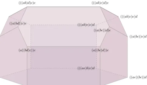
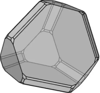
For the first two trees above, we get the 3-dimensional permutohedron and associahedron, respectively, whose edges all stand for θ-arrows in the first case, and β-arrows in the second. For the third one, we get a polytope called the hemiassociahedron, which, as we shall see, also belongs to the familly of hyper-graph polytopes. In Figure 1, we labelled some of the vertices of this polytope, matching them with decompositions of our example tree (this matching will be spelled out in Proposition 4).
(((ab)d)c)e (((ab)c)d)e ((a(bc))d)e ((a(bd))c)e (a((bc)d))e (a((bd)c))e (((ab)c)e)d ((a(bc))e)d ((ae)(bc))d (((ae)b)c)d (((ab)e)c)d
Fig. 1 The hemiassociahedron
4.2 Graphs associated with operadic trees
To every rooted tree T representing a pasting scheme for operadic operations, Doˇsen and Petri´c associate a graph G(T ), obtained as follows. Its vertices are the edges of T, and two vertices are connected whenever as edges of T they share a common vertex.
It is clear that one can identify the edges of T with the non-root nodes of T (for example, in Figure 2, there is a bijection mapping x to c, y to d, z to b, and u to e). By this identification, seeing now the nodes of G(T ) as the non-root nodes of T , all edges of T , apart from those stemming from the root, are in G(T ). All the other edges of G(T ) are edges witnessing that two edges of T are siblings. We record the latter (resp. the former) by representing them with a dashed (resp. solid) line.
The graph G(T ) is connected and can be represented itself as a tree with some horizontal dashed edges such that, by construction, each dashed horizon-tal zone is a complete graph all of whose nodes are connected to their father
a b e c d z u x y z u x y
Fig. 2 The G(T ) construction
node (if it exists) by solid edges. The nodes of G(T ) are thus organised in levels. We say that G(T ) has a root when there is no horizontal dashed layer at the bottom of G(T ).
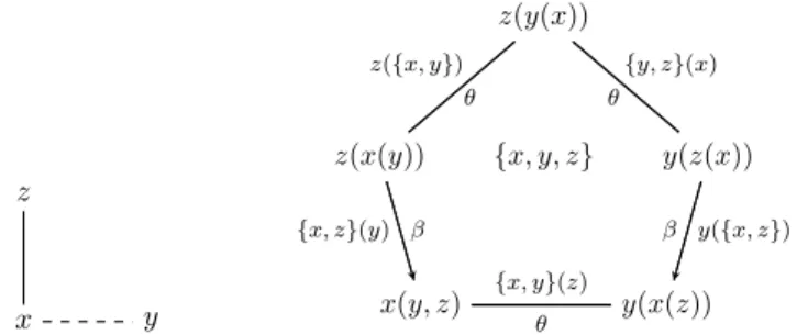
Figure 2 shows the graph associated to the third tree considered at the end of Section 4.1 (z, u are at level 1, and x, y are at level 2).
We insist that the dashed/solid informations on the edges of G(T ) are not part of the graph structure G(T ): they are additional data that we shall use to derive both the type (β or θ) and (in the case of β) the orientation of all edges of the corresponding polytope (as dictated by T ).
Recall that, in the language of constructs, vertices are trees whose nodes are all labelled with singletons. An edge E is a tree whose nodes are all singletons, except one, which is a two-element set {uE, vE}. We will show that G(T ),
together with its bipartition of dashed and solid edges, determines the type (and the orientation) of E. Let us call a min-path of a graph a path of minimum length between two vertices (we will show that in G(T ) min-paths are always unique). Our criterion is the following:
† If the min-path between uE and vE in G(T ) is made only of solid edges,
E corresponds to a β-arrow, oriented towards the vertex of E in which the label uE appears below the label vEif and only if the level of uE is inferior
to the level of vE in G(T ). Otherwise, E witnesses a θ-arrow.
As an example, let us derive the edge information for the mixed pentagon (4), out of the associated graph:
z y x z(y(x)) z(x(y)) y(z(x)) x(y, z) y(x(z)) {x, y, z} z({x, y}) θ {y, z}(x) θ {x, z}(y) β β y({x, z}) {x, y}(z) θ
According to the criterion, the orientation of, say, the β edge connecting z(x(y)) and x(y, z) is dictated by the fact that x is below z in G(T ). The orientation of the θ edges is then determined after choosing a starting vertex (one of the three upper vertices).
We now embark on the proof of soundness and completeness of this crite-rion. We shall formulate the criterion in different ways, and we shall exhibit the relationship between the connectedness properties of T and of G(T ).
We first observe that for any two distinct vertices u, v of G(T ), exactly one of the following two situations occurs (referring to u, v as edges of T ):
• Type I: u is above v or conversely.
• Type II: u and v are situated in disjoint branches of a subtree of T . We will denote by meet (u, v) the node of T at which the two branches diverge. We can reformulate these two situations in G(T ), without reference to T :
• Type I: There is a descending path of solid edges (i.e., the level decreases by 1 at each node in the path) from u to v or from v to u (such a path will be called of type I);
• Type II: There exists a path p = p1, u0, v0, p2from u to v whose parts p1, u0
and v0, p2 are descending and ascending, respectively (and therefore are
made of solid edges only) and which is such that (u0, v0) is a dashed edge (such a path will be called of type II).
That this indeed is a reformulation is obvious for type I, while for type II, the desired path in G(T ) is obtained by going down in T from (the child vertex of) u all the way down to u0 whose father node is meet (u, v), then through a dashed arrow to the branch carrying v0, and then all the way up to (the child vertex of) v. Conversely, transcribing the path p1, u0, v0, p2in the language of
T , we find a configuration of type II there.
In the next lemma, we show how to transform any path into a path of type I or II with the same end nodes. The transformations are specified by the following picture: z x y y x z z x y x y z ↓ ↓ ↓ ↓ x z x z z x x z
This specification is then used to define a rewriting system: p1, x, y, z, p2−→ p1, x, z, p2
when x, y, z are in one of the four configurations at the top of the picture. Lemma 11 This rewriting system is confluent and terminating. It is complete in the sense that any two paths between the same pair of end points are provably equal by a zigzag of such rewritings, and sound in the sense that any such zigzag always relates two paths with the same endpoints. The normal forms of the rewriting system are the paths of type I or II, and are the min-paths.
Proof. Termination is obvious, since the length decreases by 1 at each step. As for confluence, we list the critical pairs, which all admit immediate solutions (note that the sequence (x, y) solid, (y, z) dashed, (z, u) solid is excluded since one would then have x = u, which contradicts the definition of a path):
z x y u y x z u z y u x u y z x x y z u
That the paths of type I and II are in normal form is also immediate (there is no matching for the left hand sides of our rewriting rules). It remains to check that all normal forms are indeed of one of these two shapes. We proceed by induction on the length of the normal form p. Every path of length 1 is indeed of type I or II. Let now p = u, v, p1. We can assume by induction that p1is of
type I or II. There are three cases:
– (u, v) is solid with v one level up from u. Then p1cannot start with a solid
edge going down, because then p would visit u twice, nor with a dashed edge, because p would then not be a normal form. Hence p1 is of type I,
and morevoer goes up (again because otherwise p would not be a path). Then adding (u, v) in front still results in a path of type I.
– (u, v) is solid with v one down from u. Then p1 cannot start with a solid
edge going up, since p would not be in normal form. Hence prefixing p1
with (u, v) yields a path of type I (resp. II) if p1 was of type I (resp. II).
– (u, v) is dashed. Then p1cannot start with a dashed edge nor a solid edge
going down, as p would then not be in normal form. Hence p1 has to be of
type I, going up, which makes p a path of type II.
We now prove completeness. We have already observed the uniqueness of the paths of type I or II. Since we have established that the normal forms are the paths of type I or II, it follows that all paths in normal form from u to v coincide (notation ≡), and we have, for any two paths p1, p2 from u to v, and
writing nf (p) for the normal form of a path p
p1−→∗nf (p1) ≡ nf (p2)∗←− p2
Conversely, the rewriting system leaves the endpoints of the path unchanged at each step, and hence any zigzag maintains this inviariant, which establishes soundness.
That every minpath is normal is clear, since any rewriting step decreases the length of a path. For the converse, we use completeness. Suppose that p is normal, but is not a min-path, and let p1 be a min-path with the same
endpoints as p. By completeness, there exists a zigzag between p and p1, or
equivalently, by confluence, p and p1 have the same normal form. But nf (p1)
has a fortiori a length strictly smaller than p = nf (p): contradiction. ut Summing up, the following are characterisations of “being of type I or II”, for two distinct vertices u, v of G(T ) (or equivalently, two edges u, v of T ):
Type I Type II
u, v are one above the other in T u, v are on disjoint branches of a subtree of T
u, v connected by a path of type I u, v connected by a path of type II min-path between u, v is of type I min-path between u, v is of type II min-path between u, v contains min-path between u, v contains only solid edges at least one dashed edge
Indeed, by Lemma 11, we know that the min-paths are exactly the paths of type I or II, and crossing or not a dashed edge is what distinguishes among min-paths those that are of type II or I, respectively.
Lemma 12 There is a one-to-one correspondence between the subtrees of T and the connected subsets of G(T ).
Proof. The connected subset of G(T ) corresponding to a subtree T0 of T is precisely G(T0). In the other direction, let K be a connected subset of G(T ). By connectedness, for any u, v in K there exists a path p from u to v that is included in K. By Lemma 11, we know that nf (p) is also included in K. By this observation, through the transcription in T of paths of type I or II of G(T ), we conclude that the subgraph of T whose edges are precisely the
vertices of K is a subtree. ut
In what follows, in the context of operadic trees, we shall say that a tree is non-Empty if it contains at least one edge (whence the capital “E”). Clearly, all operadic trees relevant for describing operadic laws are non-Empty. Lemma 13 If x1, . . . , xn are arbitrary distinct edges of T , then the following
claims hold.
1. By removing x1, . . . , xn from T , we obtain exactly n + 1 subtrees of T .
2. The number k of non-Empty subtrees of T obtained in this way is equal to the number of connected components of G(T ) obtained by removing the vertices x1, . . . , xn, and k ∈ {0, . . . , n + 1}.
3. Let T0 be one of the non-Empty subtrees of T obtained by removing x1, . . . ,
xn, and let K be the connected subset of G(T ) associated with T by (2).
Then, if y is an edge of T0 and a vertex of K, we have that G(T0) = K. Proof. We consider only the case n = 1 (the general case follows easily by induction), and we write x for x1. Let a and b be the vertices adjacent to x,
with a being the child vertex for b.
The first claim is standard: the subtrees obtained after the removal of x are the subtree T1 rooted at a and containing all descendants of a, and the
subtree T2obtained from T by removing all of T1. Note that b is a leaf of T2.
We prove the other two claims in parallel, by looking at the possible con-figurations of T . If x is the only edge of T , then T1 and T2 are the vertex a
and the vertex b, respectively, and, therefore, k = 0. Suppose that x is not the only edge of T . Then, if x is on the highest level in T , T1is just the vertex a,
while T2is clearly non-Empty, and, hence, k = 1. We also get k = 1 when x is
the unique edge on the first level of T , in which case T1is non-Empty and T2
is just the vertex b. In all other situations, we have k = 2.
Let us now prove that k is also the number of connected components of G(T ) obtained by removing the vertex x. We examine only the case k = 2. Let K1= G(T1) and K2= G(T2). Since K1and K2are connected and disjoint and
G(T )\{x} = K1∪ K2, we only have to show that the set of edges of G(T )\{x}
is also the (disjoint) union of sets of edges of K1 and K2. For this, we use the
fact that the removal of x from G(T ) involves the removal of all edges of G(T ) that have x as one of its adjacent vertices. Let e be an edge of G(T ), with y and z being its adjacent vertices.
Suppose first that e is an edge of G(T )\{x}. We then know that both y and z are different from x, and share a common vertex v when considered as edges of T . Since T1and T2 form a partition of the set of vertices of T , let us
assume, say, that v is a vertex of T1. If v 6= a, we can immediately conclude
that y and z are edges of T1, and, if v = a, then, since both y and z are
different from x, it must be the case that v is the parent vertex for both y and z, which also implies that y and z are edges of T1. Therefore, y and z are both
vertices of K1, and, hence, e is an edge of K1.
Conversely, if e is an edge of K1, then y and z are edges of T1, and therefore
must both be different from x. Since they share a common vertex in T1, and,
hence, in T , we conclude that e is an edge of G(T )\{x}. ut The following proposition is only implicit in [5].
Proposition 4 For every operadic tree T , the constructions of G(T ) (consid-ered as hypergraph) are in one-to-one correspondence with the (fully) paren-thesised words that denote decompositions of T .
Proof. To every decomposition/parenthesisation of T , one can associate a tree each of whose nodes is decorated by an edge of T : one proceeds from the most internal parentheses to the most external ones, recording each insertion on the way.
Formally, the fullly parenthesised words are declared by the syntax w :: a || (ww), where a ranges over the nodes of T (all named with different letters).
Not all words correspond to decompositions of T . When this is the case, we say that w is admissible for T (the precise definition of admissibility can be easily reconstructed from the inductive construction below).
Since we deal with non-Empty trees, our base case is that of a word (ab) corresponding to a single edge operadic tree connecting a and b. Then there is only one decomposition and one construction, hence the statement holds.
Otherwise, we have a word w = (w1w2), where at least one of the words
w1or w2is not reduced to a letter. We proceed by structural induction on w,
providing both the decorated tree and the proof that is indeed a construction. Let us call T1, T2 the trees decomposed by w1, w2, respectively (cf. Lemma
13). Let x be the edge on which T1 is grafted on the tree T2. We distinguish
three cases.
1. If neither w1nor w2are reduced to a letter, then G(T1) and G(T2) are both
non-empty, and are the connected components of G(T )\{x}. We can thus apply induction: if V1and V2are the constructions associated with w1and
w2, then we associate x(V1, V2) with (w1w2), which is a construction.
2. If w2= a is a reduced to a letter and w1 is not reduced to a letter, then
G(T2) is empty, and x is a leaf of G(T ). We conclude by induction that the
tree x(V1) associated with ((w1)a) is a construction.
3. If w1= a is reduced to a letter, then T is of the form a(T2), i.e. a is the root
and has only one child which is the root of T2. We conclude by induction
that the tree x(V2) associated with (a(w2)) is a construction.
Note that case 1 (resp. cases 2 and 3) correspond to the situation where k = 2 (resp. k = 1), while the base case is the case where k = 0 (in the terminology of Lemma 13).
The converse mapping is defined much in the same way. We observe that, for any T (with at least 3 nodes), constructions of G(T ) can only be of the form x(V ) or x(V1, V2). They are of the first (resp. second) form when the
node x is either a leaf or the root of G(T ), (resp. when x is any other node). We can deploy induction on the number of nodes of T and map constructions back to parenthesised words. By induction too, we can show that these are
inverse transformations. ut
As an illustration, referring to Figure 2, (ae)((bd)c) is mapped to z(x(y), u), obtained as follows: the leaf u records ae, while in parallel the leaf y records bd and then x(y) encodes (bd)c and, finally, the last insertion is along z. (Note that, following common practice, in examples, we do not write the most ex-ternal parentheses.)
We are now in a position to conclude.
Theorem 2 The criterion (†) is sound and complete.
Proof. We write u, v for uE, vE. Let E0 be the subtree of E whose root is
{u, v} and let K be the connected subset of G(T ) out of which E0 arises as a
construct. Let T0 be the subtree of T that corresponds to K by Lemma 12.
The number of constructions grafted to {u, v} in E0 is the number of con-nected components of K\{u, v}. By Lemma 13, it is also the number of non-Empty subtrees of T0obtained by removing the edges u and v. Moreover, there can be at most 3 such subtrees. Let us now introduce some names.
Let T10, T20 and T30 be the subtrees of T0 obtained by removing u and v. Let I ⊆ {1, 2, 3} be such that i ∈ I if and only if Ti0 is non-Empty, and let J = {1, 2, 3}\I. Let, for all i ∈ I, Kibe the connected component of K\{u, v}
corresponding to Ti0, Vi be the construction of Ki that is grafted to {u, v}
in E0, and wi be the decomposition of Ti0 corresponding to Vi according to
Proposition 4. On the other hand, for all j ∈ J , Tj0 is a vertex aj, and let wj