Collision Avoidance System Optimization for
Closely Spaced Parallel Operations through
Surrogate Modeling
by
Kyle A. Smith
B.S., United States Air Force Academy (2011)
Submitted to the Department of Aeronautics and Astronautics
in partial fulfillment of the requirements for the degree of
Master of Science in Aeronautics and Astronautics
at the
MASSACHUSETTS INSTITUTE OF TECHNOLOGY
June 2013
This material is declared a work of the U.S. Government and is not
subject to copyright protection in the United States.
Author . . . .
Department of Aeronautics and Astronautics
April 10, 2013
Certified by . . . .
Mykel J. Kochenderfer
Technical Staff, Surveillance Systems Group, MIT Lincoln Laboratory
Thesis Supervisor
Certified by . . . .
Jonathan P. How
Richard C. Maclaurin Professor of Aeronautics and Astronautics
Thesis Supervisor
Accepted by . . . .
Eytan H. Modiano
Professor of Aeronautics and Astronautics
Chair, Graduate Program Committee
Disclaimer:
The views expressed in this thesis are those of the author and do not reflect the official policy or position of the United States Air Force, Department of Defense, or
Collision Avoidance System Optimization for Closely Spaced
Parallel Operations through Surrogate Modeling
by
Kyle A. Smith
Submitted to the Department of Aeronautics and Astronautics on April 10, 2013, in partial fulfillment of the
requirements for the degree of
Master of Science in Aeronautics and Astronautics
Abstract
The Traffic Alert and Collision Avoidance System (TCAS) is mandated worldwide to protect against aircraft mid-air collisions. One drawback of the current TCAS design is limited support for certain closely spaced parallel runway operations. TCAS alerts too frequently, leading pilots to often inhibit Resolution Advisories during approach. Research is underway on the Airborne Collision Avoidance System X (ACAS X), a next-generation collision avoidance system that will support new surveillance systems and air traffic control procedures. ACAS X has been shown to outperform TCAS for enroute encounter scenarios. However, the design parameters that are tuned for the enroute environment are not appropriate for closely spaced parallel operations (CSPO).
One concept to enhance the safety of CSPO is a procedure-specific mode of the logic that minimizes nuisance alerts while still providing collision protection. This thesis describes the application of surrogate modeling and automated search for the purpose of tuning ACAS X for parallel operations. The performance of the tuned system is assessed using a data-driven blunder model and an operational performance model. Although collision avoidance system development normally relies on human judgment and expertise to achieve ideal behavior, surrogate modeling is efficient and effective in tuning ACAS X for CSPO as the tuned logic outperforms TCAS in terms of both safety and operational suitability.
Thesis Supervisor: Mykel J. Kochenderfer
Title: Technical Staff, Surveillance Systems Group, MIT Lincoln Laboratory
Thesis Supervisor: Jonathan P. How
Acknowledgments
I would like to thank MIT Lincoln Laboratory for supporting my education and research over the past two years, especially Col. (ret) John Kuconis, Division 4 Di-rector Dr. Israel Soibelman, Group 42 Leader Gregory Hogan, and Associate Group 42 Leader Dr. Gregg Shoults.
I am thankful for Dr. Wesley Olson’s leadership and support as head of the Group 42 ACAS X program, and for continually guiding and supporting my work in every aspect. This work was sponsored by the FAA TCAS Program Office AJM-233, and I gratefully acknowledge Neal Suchy for his leadership and support.
I am extremely grateful to Professor Jonathan How as my advisor and thesis supervisor for looking out for my best interests over the past two years and ensuring that I stayed on target in successfully completing my coursework and research on time.
I am indebted to Dr. Mykel Kochenderfer for his continual guidance during my en-tire time at Lincoln Laboratory, including helping to provide direction for my research and invaluable critique of this thesis throughout the entirety of its development. Like-wise, Dr. Adan Vela stood by my side during critical moments of research and writing and dedicated extensive effort and time to helping me complete quality work. I would not have succeeded without the hard work and commitment exhibited by these two gentlemen.
I am thankful to numerous members of Group 42 and others within Lincoln Lab-oratory who offered their expertise when I needed it most. Specifically, I wish to thank Jessica Holland, Dylan Asmar, James Chryssanthocopoulos, Tomas Elder, and Thomas Billingsley for their insights and assistance in completing this work. Chung Lee of Georgia Tech was a great help due to his early input regarding potential opti-mization tools. I am also appreciative of my officemate Melvin Stone for his seemingly endless supply of stories, advice, peanuts, and tea.
Finally, the love and support shown by my family and friends never ceases to amaze me. Throughout the years, they have played a critical role in building the foundations for who I am today and every one of my accomplishments, and I am forever grateful.
Contents
1 Introduction 11
1.1 Traffic Alert and Collision Avoidance System . . . 11
1.2 Closely Spaced Parallel Operations . . . 14
1.3 Collision Avoidance System Design . . . 17
1.4 ACAS X . . . 19
1.5 Objective: Tuning ACAS Xo for CSPO . . . 20
1.6 Literature Review: Optimization Methods . . . 21
1.7 Contributions and Outline . . . 23
2 Worst-Case Analysis of Airborne Collision Avoidance Systems 25 2.1 Problem Description . . . 26
2.2 Worst-Case Analysis . . . 30
2.3 Discussion . . . 35
3 Optimization via Surrogate Modeling 37 3.1 Performance Metrics . . . 38
3.2 Historical Encounter Set . . . 39
3.3 Simulation and Evaluation . . . 42
3.4 Defining the Objective Value . . . 43
3.5 Screening Study . . . 44
3.6 Sampling Plan . . . 46
3.7 Surrogate Modeling . . . 47
3.9 Discussion . . . 53
4 Performance Analysis 55 4.1 Historical Encounter Set Performance . . . 57
4.2 Individual Parameter Analysis . . . 61
4.3 Generated Encounter Set Performance . . . 63
4.4 Operational Performance Analysis . . . 68
4.5 Policy Examples . . . 73
4.6 Application of Worst-Case Analysis to ACAS Xo Development . . . . 76
4.7 Discussion . . . 82
5 Conclusions and Further Work 85
A Objective Value Weighting Sweep 89
List of Figures
1-1 Example TA cockpit display and annunciation . . . 12
1-2 Example RA cockpit display and annunciation . . . 12
1-3 Aircraft trajectories and TCAS commands in the ¨Uberlingen mid-air collision . . . 13
1-4 Example parallel approach scenario . . . 15
1-5 Example dependent approach geometry . . . 16
1-6 Example overtake geometry . . . 16
1-7 Example oscillation geometry . . . 17
1-8 Example TCAS pseudocode . . . 18
1-9 Example slow-closure geometry . . . 19
1-10 ACAS X optimization and development process . . . 20
2-1 Encounter timeline . . . 27
2-2 Climb maneuver . . . 28
2-3 Constant-drift blunder . . . 28
2-4 Constant-turn blunder . . . 29
2-5 Worst-case available time to alert (tc) vs. drift angle . . . 31
2-6 Drift angle vs. perpendicular deviation . . . 32
2-7 Worst-case available time to alert (tc) vs. turn rate . . . 33
2-8 Worst-case available time to alert (tc) vs. turn rate . . . 34
2-9 Turn rate vs. perpendicular deviation . . . 34
3-1 Overview of the optimization via surrogate modeling process . . . 38
3-3 Example aircraft behavior . . . 41
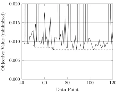
3-4 Objective values of eighty infill points (solid) and the cumulative min-imum value achieved (dashed) . . . 51
4-1 Sample encounter . . . 60
4-2 Sample encounter . . . 61
4-3 Effect of cycles parameter . . . 63
4-4 Generated encounter set configuration . . . 65
4-5 Probability (in percent) of alert . . . 69
4-6 No-blunder CSPO configuration (vertical sweep) . . . 73
4-7 Example policy plots for Aircraft 1 . . . 74
4-8 No-blunder CSPO configuration (horizontal sweep) . . . 75
4-9 Example horizontal alert probabilities for Aircraft 1 . . . 75
4-10 Sample encounter . . . 77
4-11 Sample encounter . . . 78
4-12 Sample encounter . . . 79
4-13 Sample encounter . . . 80
4-14 Worst-case available time to alert (tc) vs. drift angle; Actual ACAS Xo alert time vs. drift angle . . . 81
4-15 Worst-case available time to alert (tc) vs. turn rate; Actual ACAS Xo alert time vs. turn rate . . . 81
A-1 Risk ratio (blue) and nuisance alert rate (red) at the optimal point found for each weighting combination . . . 101
List of Tables
3.1 Optimization Performance Metrics . . . 39
3.2 Design Parameters Analyzed in the Screening Study . . . 44
3.3 Design Parameter Screening Study Results (Mean) . . . 45
3.4 Design Parameter Screening Study Results (Standard Deviation) . . . 45
3.5 Design Parameter Ranges used for Optimization . . . 47
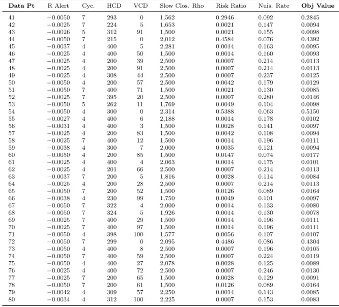
3.6 Evaluation Results for the First Forty Infill Points . . . 52
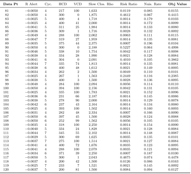
3.7 Evaluation Results for the Second Forty Infill Points . . . 53
4.1 ACAS Xo Parameter Value Changes Relative to ACAS Xa . . . 56
4.2 Metric Results for the Historical Blunder Encounter Set . . . 58
4.3 Metric Results using ACAS Xa Settings for One Parameter at a Time 62 4.4 Metric Results for the Generated Blunder Encounter Set . . . 66
4.5 Metric Results for the Generated Nominal Encounter Set . . . 67
A.1 Evaluation Results for the First Forty Infill Points (97.5%/2.5%) . . . 91
A.2 Evaluation Results for the Second Forty Infill Points (97.5%/2.5%) . 92 A.3 Evaluation Results for the First Forty Infill Points (92.5%/7.5%) . . . 93
A.4 Evaluation Results for the Second Forty Infill Points (92.5%/7.5%) . 94 A.5 Evaluation Results for the First Forty Infill Points (90%/10%) . . . . 95
A.6 Evaluation Results for the Second Forty Infill Points (90%/10%) . . . 96
A.7 Evaluation Results for the First Forty Infill Points (85%/15%) . . . . 97
A.8 Evaluation Results for the Second Forty Infill Points (85%/15%) . . . 98
A.9 Evaluation Results for the First Forty Infill Points (80%/20%) . . . . 99
List of Acronyms and Abbreviations
ACAS Airborne Collision Avoidance System
CAT Category
CSPO Closely Spaced Parallel Operations
deg degrees
ft feet
ILS Instrument Landing System
IMC Instrument Meteorological Conditions
kt knots
lbs pounds
Max EI Maximum Expected Improvement
min minute
MLE Maximum Likelihood Estimate
NAS National Airspace System
NextGen Next Generation Air Transportation System
NM Nautical Mile
NMAC Near Mid-Air Collision
NTZ No Transgression Zone
PRM Precision Runway Monitor
RA Resolution Advisory
RNP Required Navigation Performance
TA Traffic Alert
Chapter 1
Introduction
This thesis asserts that a surrogate modeling and automated search process can tune an airborne collision avoidance system for ideal alerting behavior during closely spaced parallel operations (CSPO). The goal is to produce a system that maintains or en-hances the safety level of the current operational system while reducing unnecessary alerts, thereby decreasing pilot workload during parallel approaches. Improved alert-ing behavior will allow for greater operational efficiency duralert-ing CSPO, leadalert-ing to greater airport throughput and cost savings especially during Instrument Meteoro-logical Conditions in which pilots and controllers cannot rely on visual separation between aircraft.
1.1
Traffic Alert and Collision Avoidance System
The Traffic Alert and Collision Avoidance System (TCAS) provides pilots with verti-cal avoidance maneuver guidance when a near mid-air collision is imminent. TCAS is currently mandated on all commercial aircraft with more than thirty seats or a max-imum takeoff weight greater than 33,000 lbs, in addition to being used extensively by many business jet type aircraft [9]. TCAS is able to provide pilots with both Traf-fic Alerts (TAs) and Resolution Advisories (RAs) for any aircraft with an operating transponder. TAs warn pilots of nearby traffic that poses a potential threat and fa-cilitate pilots in visually acquiring the traffic. TAs consist of an aural annunciation
(“Traffic, Traffic”) and traffic information such as relative altitude on a visual display in the cockpit, as depicted in Figure 1-1.
Figure 1-1: Example TA cockpit display and annunciation
Figure 1-2: Example RA cockpit display and annunciation
If a threat becomes imminent, an RA is issued to prevent a collision by command-ing the pilot to execute a vertical avoidance maneuver (e.g., Climb, Descend, Level
Off). As shown in Figure 1-2, RAs include visual instructions such as target vertical speeds or pitch angles, as well as aural annunciations (e.g., “Climb, Climb”). TCAS functions independently of ground-based systems and air traffic controllers and relies on surveillance equipment onboard the aircraft [9].
If an aircraft has begun a maneuver in concordance with an RA, the ground con-troller is no longer responsible for separation between that aircraft and any other aircraft, airspace, or obstacle. Once the controller is aware of the RA, he or she is not authorized to instruct the pilot to maneuver contrary to the RA. Controller responsibility for separation is reinstated when either the aircraft returns to its pre-viously assigned altitude or the pilot indicates that the RA maneuver is completed. The pilot in command is ultimately responsible for the safe operation of flight and should immediately respond to any RA unless a response would jeopardize safety or is deemed unnecessary by visual contact with the target aircraft [9]. To illustrate the importance of these responsibilities, Figure 1-3 shows the aircraft trajectories and TCAS commands in the 2002 mid-air collision over ¨Uberlingen, Germany. The con-flicting instructions of TCAS (Climb) and air traffic control (Descend) resulted in the Russian Tu-154 passenger jet following the controller’s instructions and descending into the path of the Boeing B-757 [23].
Figure 1-3: Aircraft trajectories and TCAS commands in the ¨Uberlingen mid-air collision [23]
1.2
Closely Spaced Parallel Operations
The National Airspace System (NAS) is operated by the Federal Aviation Adminis-tration and consists of various units that regulate, coordinate, and supervise aircraft travel over the United States. The NAS is designed to enable safe and efficient air-craft operations through the interaction of airspace structure, technologies, policies, and standard procedures [40]. One such set of procedures is CSPO, in which multi-ple aircraft simultaneously approach parallel runways for landing at a given airport to increase airport throughput. Depending on the airport, parallel runways can be laterally spaced as close as 700 ft [28]. Uninterrupted and efficient CSPO is normally feasible during Visual Meteorological Conditions when pilots are able to maintain vi-sual separation with other aircraft. However, Instrument Meteorological Conditions (IMC) are defined by varying degress of reduced visibility and cloud clearance, de-pending on the type of airspace. As visibility deteriorates in IMC, safety cannot be ensured at smaller runway spacings and CSPO is restricted to a smaller set of runway configurations. This limited CSPO capability decreases airport throughput, causes delays in the air and on the ground, and decreases the overall efficiency in the NAS [7].
Executing CSPO often allows for higher airport throughput than would otherwise be achievable [7]. However, such operations are sometimes prohibited due to safety concerns, such as during IMC. Between October 2010 and March 2011, CSPO ac-counted for 13% of all unique RAs detected in U.S. high-tempo regions. Among the most affected regions were San Francisco, where 92.6% of RAs were during parallel approaches, Atlanta (56.3%), and Denver (54.1%) [28]. Under current regulations, independent parallel approaches, in which no minimum diagonal spacing is required, may only be conducted in IMC for runways separated laterally by at least 4300 ft [25]. This requirement is relaxed down to a minimum of 3000 ft if certain conditions are met for approaches equipped with the Precision Runway Monitor (PRM) system. PRM employs a ground-based high-update-rate radar that allows an air traffic controller to closely monitor aircraft tracks on parallel approaches. If either aircraft deviates, or
blunders, from its correct trajectory into a predefined No Transgression Zone (NTZ) during PRM, as illustrated in Figure 1-4, the controller will issue an alert to prevent a collision if TCAS has not already issued an RA [3]. These separation standards were developed by simulating worst-case blunder scenarios and determining the minimum acceptable runway separations [25].
Runway Stagger No Transgression Zone (NTZ) 2000 ft Runway thresholds Turn onto localizer Glide slope capture
Figure 1-4: Example parallel approach scenario
PRM is only available at select U.S. airports and only allows dependent ap-proaches, in which aircraft must maintain certain diagonal spacing in addition to in-trail spacing, for runway separations of at least 3000 ft [25]. Figure 1-5 gives an example of this dependent approach geometry.
Figure 1-5: Example dependent approach geometry [2]
PRM also requires an additional specially trained controller to monitor and pro-vide separation assurance for the aircraft on parallel approach. This staffing require-ment can be difficult to schedule, especially in the case of unanticipated weather events. Providing an alternate means of conducting CSPO in IMC for smaller run-way separations, specifically an enhanced airborne collision avoidance system, would enable high throughput at a larger set of airports without requiring additional staffing or technology on the ground.
CSPO often involves unique aircraft geometries that require collision avoidance logic to respond with fine-tuned sensitivity. One example is an overtake scenario, shown in Figure 1-6, in which a trailing aircraft overtakes a lead aircraft on a parallel approach due to speed differential.
Figure 1-6: Example overtake geometry [9]
A second example involves navigation error during CSPO in IMC. For instance, an aircraft may appear to be initiating a blunder toward another aircraft on approach, as shown in Figure 1-7, but it may simply be oscillating along the approach path while
attempting to stabilize its track along the localizer during an Instrument Landing System (ILS) approach.
Figure 1-7: Example oscillation geometry
As a third example, an aircraft that seems to be aimed toward another aircraft on final approach may simply be angling to initially establish the localizer, as in Figure 1-4. These situations are typically safe and intentional, but the challenge lies in tuning the collision avoidance system such that it can distinguish between these safe scenarios and imminent threats due to deviations from the correct nominal flight paths.
1.3
Collision Avoidance System Design
There are a number of trade-offs that must be taken into account in the design of a collision avoidance system. For example, the system should alert frequently enough to maintain a desired level of safety. However, the system should also minimize nuisance alerts such that safe operations can be performed without being interrupted by an RA. There are several hazards associated with nuisance alerts. For example, when faced with too many unnecessary alerts during intentional and safe operations, pilots may become desensitized and distrust the collision avoidance system, potentially ignoring legitimate alerts [23, 31].
Collision avoidance systems are highly complex and a comprehensive understand-ing of their decision processes is not a trivial task for most common users. The fact
that pilots regularly utilize collision avoidance systems “implies that they must have made a leap of faith” [27]. This leap of faith is heavily based on experience with the system and its perceived predictability during risky events, leading the pilot to generalize the system’s dependability [24]. Perceived system unreliability can also lead to increased response times due to indecision about the best course of action [33]. Finally, excessive nuisance alerts may increase the potential for induced colli-sions where a pilot follows a nuisance RA, maneuvers unnecessarily, and creates an unsafe situation.
Figure 1-8: Example TCAS pseudocode [34]
TCAS follows a complex set of heuristic rules, as illustrated in the pseudocode of Figure 1-8, that are difficult to adjust in concordance with airspace and proce-dure changes over time. At its foundation, the TCAS logic uses the projected time until closest point of approach to determine when to issue an RA. However, during slow-closure situations, such as in Figure 1-9, the projected time until closest point of approach may be too large to provide adequate protection against an intruder air-craft. In these circumstances, TCAS uses an enlarged critical region based on the aircraft altitude. These ranges are defined as follows: 0.2 NM below 2350 ft Above
Ground Level, 0.35 NM below 5000 ft Mean Sea Level, and 0.55 NM between 5000 ft and 10,000 ft Mean Sea Level [9]. Although the thresholds defining the critical re-gion tend to provide an adequate level of safety, rigid rules like these can result in undesirable alert rates and behavior during CSPO [23, 30, 37].
Figure 1-9: Example slow-closure geometry [9]
1.4
ACAS X
As the airspace evolves with the introduction of the Next Generation Air Trans-portation System (NextGen), research is underway to field a system known as the Airborne Collision Avoidance System X (ACAS X) to replace TCAS. In contrast to the rule-based logic of TCAS, ACAS X uses probabilistic models and cost functions to determine an optimal collision avoidance action [21]. Four variants of ACAS X are in development for different users and objectives. The first variant is ACAS Xa, which uses active secondary radar supplemented with passive surveillance. ACAS Xa is the analogue to TCAS and is intended to be used by current TCAS-mandated users during the majority of flight operations. ACAS Xo, the subject of this thesis, is tuned for specific operations such as CSPO. ACAS Xo issues procedure-specific RAs for designated aircraft while ACAS Xa maintains global protection against all other aircraft in the vicinity. The initial version of ACAS Xo uses the same surveillance as ACAS Xa, while future versions may incorporate data obtained directly from other aircraft such as bank angle or autopilot status. The two other variants, ACAS Xp
and Xu, are designed for general aviation aircraft and unmanned aicraft, respectively. The optimization and development process of ACAS X is depicted in Figure 1-10 [21]. ACAS X differs from TCAS in that it uses a probabilistic dynamic model of aircraft behavior and optimizes the alerting behavior with respect to an offline cost function defined by numerous design parameters (approximately forty). The aim of the cost function is to balance safety and operational goals such as minimizing collision risk and nuisance alerts. With an appropriate cost function and probabilistic model, a dynamic programming approach is used to precompute an offline look-up table and optimal system parameters (millions). Using the offline look-up table and additional online parameters in real-time, the optimal action is determined at each timestep.
Probabilistic Dynamic Model Offline Look-up Table Dynamic Programming Onboard Logic Offline Design Parameters Online Design Parameters
Figure 1-10: ACAS X optimization and development process
1.5
Objective: Tuning ACAS Xo for CSPO
CSPO is the initial target application for ACAS Xo. The goal of ACAS Xo is to provide additional protection during CSPO, especially in IMC, while minimizing un-necessary alerts. Providing protection with minimal alerting will increase the effi-ciency of parallel approaches during IMC and help achieve NextGen goals such as fewer flight delays, greater cost savings, and increased throughput at high-volume airports [17]. TCAS has been able to maintain adequate safety levels during CSPO [23], but it is also plagued with excessive alert rates which cause pilots to inhibit RAs by switching to a TA-only mode [28]. To be operationally suitable for CSPO, ACAS Xo must maintain the safety level of TCAS while improving the overall alerting behavior, specifically by reducing nuisance alerts.
The performance of ACAS Xo depends on design parameters that can be tuned to modify various behaviors of the collision avoidance logic. Hand-tuning these design parameters is challenging since the impact of changing parameters can be difficult to predict, usually resulting in sub-optimal system behavior. Instead, optimization via surrogate modeling is applied to tune parameters for desirable ACAS Xo performance during CSPO. The safety and alerting performance of ACAS Xo on a set of CSPO encounters is essentially a “black-box” function that is dependent on the individual design parameter values. Using surrogate modeling to tune ACAS Xo allows for a more efficient and effective process that results in ideal alerting behavior during CSPO encounters.
The global optimization process used here efficiently selects data points to test in order to model the “black-box” function that is unknown to the user [11]. The function value at a given point is unknown until a simulation is performed for a certain combination of parameter settings. Exploring the design space improves the function prediction, thereby allowing the search method to identify promising areas of the design space (i.e., parameter settings) to search [18]. Eventually the design space is explored thoroughly enough to determine the location of the global optimum. The objective of this thesis is to apply the aforementioned global optimization to ACAS Xo such that it achieves acceptable performance on the encounter set used for tuning as well as additional independent CSPO encounter sets that represent various aircraft behaviors and procedures. Furthermore, the tuning process should result in ACAS Xo outperforming TCAS in terms of both safety and operational suitability in all encounter sets used for analysis.
1.6
Literature Review: Optimization Methods
Variations of this global optimization process have been used in many different ap-plication areas. One example is a model for flame velocity (output) based on five different chemical reaction rates (input). The objective was to tune a computer fluid-dynamics model to match physical data for flame velocity. High computational cost
for each run dictated the need for careful selection of data points to test [35]. Another application has been in minimizing the drag coefficient of an airfoil (output) defined by various inputs such as thickness-to-chord ratio. Expensive computer simulations must be run to determine the drag coefficient at each distinct input setting [10].
There are many different types of surrogate models that can be used for tuning. Kriging models are often used due to the flexibility and high dimensionality that they allow. Kriging was originally developed for geostatistics, where core samples were taken at carefully selected positions with the goal of predicting the concentration of a mineral at a given location [18]. The model has been applied to a wide range of topics and represents a special case of radial basis functions. The Kriging model is used extensively in work by Forrester et al., Jones et al., Sacks et al., and Schonlau, who sometimes refer to the model as a “stochastic process model” [10, 11, 18, 35, 36]. Sacks et al. explored various methods of determining the Kriging model parameters that best represent a given data set, including Integrated Mean Squared Error and Maximum Mean Squared Error [35].
Jones et al. developed a process called “Efficient Global Optimization” which uses a Kriging model and search criteria that maximizes expected improvement for each evaluation point [18]. Forrester et al. expanded the scope of global optimization work by applying Kriging and max expected improvement criteria to noisy computer exper-iments and adjusting the estimate of prediction error [10, 11]. Regis and Shoemaker developed a global optimization method subject to nonlinear constraints. Additional constraints were imposed which force the search method to cycle between global and local search by specifying the next evaluation point’s minimum distance from pre-vious data points [32]. This thesis mainly utilizes methods developed by Forrester et al. to show that global optimization can be used to tune ACAS Xo for optimal performance during CSPO [11].
On a broader level, there are numerous stochastic optimization methods that do not rely on an already existing model of the “black-box” function. A genetic algorithm is one such method which uses ideas derived from evolution to find an optimal solution, as outlined by Goldberg and Whitley [12, 42]. A process of selection is applied to each
population to determine the best solutions. Recombination and mutation processes are applied to the population to generate a new population that is ideally comprised of more promising solutions.
Alternatively, Kirkpatrick et al. and Press et al. describe Simulated Annealing as an optimization method that bases its implementation on thermodynamic principles [19, 29]. The goal is to navigate around many local optima within a large design space to find the approximate location of the global optimum. An annealing schedule is generated which dictates the direction and magnitude of change in parameter settings. An important feature of Simulated Annealing is that, in a minimization problem for example, the algorithm may accept sample points with higher objective values, but with decreasing probability over time.
Gaussian Adaptation is an additional optimization method that is similar to Sim-ulated Annealing with respect to the decreasing probability of accepting less desirable points over time [20]. Drawing from its name, Gaussian Adaptation adapts a Gaussian distribution to regions of feasible points in the design space. Certain regions in the design space are designated as feasible based on whether associated samples satisfy a criterion that becomes more demanding over time. This increasingly demanding criterion drives the aforementioned decreasing probability of accepting points with higher objective values (when minimization is desired).
1.7
Contributions and Outline
This thesis offers several contributions to the problem of designing airborne collision avoidance systems:
Worst-case scenarios are identified for various blunder types and severities, and the available alert time is calculated for each scenario. The worst-case available alert times help guide the development of collision avoidance systems by defining alerting requirements at various parallel approach configurations.
process for tuning collision avoidance systems. Given a collision avoidance logic dependent on a small number of design parameters, the logic’s performance can be tuned to behave optimally for specific operations and procedures.
The tuning process is shown to not only result in acceptable ACAS Xo per-formance, but also in exceptional performance on independent encounter sets compared to that of TCAS. As ACAS Xo development continues in the future, the tuning process can be reapplied to update the design parameter settings based on revised versions of the logic.
The remainder of this thesis is organized as follows:
Chapter 2 completes a worst-case analysis of CSPO. The alerting limits of col-lision avoidance systems during these worst-case scenarios are determined for varying aircraft behaviors, runway configurations, and pilot responses. These collision avoidance limits help guide the development of ACAS Xo and establish realistic expectations for performance in worst-case scenarios.
Chapter 3 provides an overview of the surrogate modeling and tuning process, as well as the encounter set used for simulations. The results of the tuning process are presented in preparation for more detailed performance analysis in Chapter 4.
Chapter 4 analyzes and compares the safety and alerting performance of TCAS and ACAS Xo. Additional encounter sets are utilized to compare TCAS and ACAS Xo alerting ranges and probabilities in certain approach configurations. Performance contributions of individual ACAS Xo parameters are analyzed, and the ACAS Xo logic is tested in various worst-case scenarios from Chapter 2. The alerting behavior of ACAS Xo is also compared to the limits determined in Chapter 2.
Chapter 5 concludes and suggests areas for further work related to the limits of collision avoidance and tuning ACAS Xo for CSPO.
Chapter 2
Worst-Case Analysis of Airborne
Collision Avoidance Systems
During CSPO, there may exist certain blunders and aircraft configurations that com-prise “worst-case” scenarios in which a collision avoidance system may be unable to alert in time to prevent a near mid-air collision (NMAC). This inability to alert in time may be caused by several factors, most notably: a small period of time between blunder initiation and NMAC, and the desire to minimize nuisance alerts. Minimizing nuisance alerts is only desirable until safety is undermined. The worst-case scenarios analyzed in this chapter aid in understanding where this threshold lies. Understand-ing the alertUnderstand-ing requirements of collision avoidance systems durUnderstand-ing CSPO is helpful in guiding the development of ACAS Xo and setting realistic expectations for its performance.
To extract certain worst-case scenarios, two types of basic aircraft blunders rel-evant to CSPO are simulated for the intruder aircraft, as well as a corresponding vertical avoidance maneuver for the own aircraft. By simulating these aircraft dy-namics within feasible parallel approach configurations, scenarios are extracted for which an NMAC is only avoidable if the collision avoidance system issues an RA within a small timeframe.
2.1
Problem Description
A general encounter framework is applied from which worst-case scenarios can be extracted. Each encounter consists of two aircraft on final approach to parallel run-ways separated by distance D. The own aircraft is defined to be on final approach to the left runway and only strays from its nominal flight path to execute a vertical avoidance maneuver. The intruder aircraft is defined to be on approach to the right runway and is simulated to blunder into the own aircraft’s flight path. Both aircraft maintain a constant speed (v1 and v2, respectively) and a 3° glide slope, with the exception of the own aircraft which may deviate from its glide slope to execute an avoidance maneuver. Only the own aircraft is simulated as equipped with a collision avoidance system, as the intruder does not terminate its blunder maneuever once initiated.
Two types of blunders are simulated: constant-drift and constant-turn. The constant-drift blunder is characterized by the intruder flying a normal final approach and suddenly altering its course to the left by a constant drift angle β. The intruder maintains its new course across the own aircraft’s approach path. The constant-turn blunder is characterized by the intruder flying a normal final approach and then initiating and maintaining a constant-rate turn to the left with turn rate ω.
The possible avoidance maneuvers for the own aircraft are limited to a constant-rate climb or descent. The own aircraft dynamics [43] are modeled such that the pilot applies a constant-acceleration control input until the target rate of climb or descent is achieved. Unless otherwise stated, the target vertical rate for climbs/descents is fixed at ±2500 ft/min since that is the greatest vertical rate commanded by TCAS and ACAS Xo. Furthermore, a 5 s pilot response delay (P D) is assumed unless otherwise stated. This delay is the elapsed time between the initial RA and the initial pilot response to the RA. For simplicity, no horizontal avoidance maneuevers are simulated. This simplification aligns with the implementation of TCAS and ACAS Xo, both of which restrict RAs to the vertical dimension [9, 21].
to alert in order to avoid an NMAC, which is defined as when aircraft come within 500 ft horizontally (hnmac) and 100 ft vertically (vnmac) of each other. This calculation requires knowledge of the theoretical time until NMAC, assuming the own aircraft does not execute an avoidance maneuver, and the time required for the own aircraft to respond to an RA and climb or descend to a clear-of-conflict altitude. These values are represented by T and tm, respectively. The difference of these two values results in the time available for the collisoin avoidance system to issue an RA before an NMAC is unavoidable, represented by tc:
tc = T − tm. (2.1)
The point at which tc= 0 indicates where an NMAC is unavoidable unless an RA is issued before the blunder is initiated. Figure 2-1 illustrates the relationship between T , tm, and tc.
Figure 2-1: Encounter timeline
Figure 2-2 illustrates an example vertical profile over time of the own aircraft (blue) and intruder aircraft (red) after the intruder has begun to blunder. After the intruder begins to blunder at time zero, the own aircraft receives an RA at time tc and initiates a climb avoidance maneuver after the pilot response delay P D. In this case, since the RA was issued at time tc, the own aircraft achieves clear-of-conflict vertical separation vnmac at time T . If the RA had been issued any later, the own aircraft would not have had enough time to maneuver to a safe altitude. If the RA had been issued earlier, separation would have been achieved with altitude to spare.
Figure 2-2: Climb maneuver
Figure 2-3 illustrates the horizontal profile of an example constant-drift blunder scenario. For the constant-drift blunder, T is defined as a quadratic such that
T = −b − √ b2− 4ac 2a , (2.2) where a = v12+ v22− 2v1v2cos(β) b = 2v2(S cos(β) − D sin(β)) − 2Sv1 c = D2+ S2 − h2 nmac.
Figure 2-4: Constant-turn blunder
Figure 2-4 illustrates the horizontal profile of an example constant-turn blunder scenario. T cannot be calculated directly for the constant-turn blunder and requires a series of intermediate steps. The intruder’s turn radius and velocity help calculate when the intruder enters and exits the horizontal region defined by a perpendicular distance of hnmac from either side of the own aircraft’s flight path. The boundaries
of this region represent the outer bounds for the possible values of T . Discretizing and searching over this time range yields the time when the intruder is first within an absolute horizontal distance of hnmac from the own aircraft.
2.2
Worst-Case Analysis
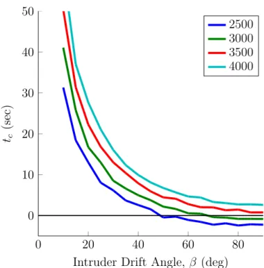
With the previous aircraft dynamics and blunders developed, an analysis of the phys-ical collision avoidance limits can be completed. For a constant-drift blunder, the minimum (worst-case) available time to alert (tc) is calculated for a given runway separation and intruder drift angle β, for 10–90° in 5° intervals, over all possible combinations of velocity, longitudinal runway stagger, and longitudinal aircraft stag-ger. The velocity for each aircraft is searched between 110 and 170 kt in 5 kt incre-ments. Longitudinal runway and aircraft stagger are both searched between =4000 and 4000 ft in 200 ft increments. The vertical aircraft stagger is not directly varied, but rather derived from the longitudinal runway and aircraft stagger distances.
Figure 2-5 displays the worst-case available time to alert (tc) versus drift angle β for a 5 s pilot response delay and runway separations of 2500, 3000, 3500, and 4000 ft. As drift angle β increases, the plot lines become slightly wavy due to the velocity and stagger discretization eliminating potentially worse scenarios from consideration. The smallest drift angle β for which the worst-case configuration precludes NMAC resolution (tc < 0) is 50° at 2500 ft runway separation. The worst-case scenario at 3000 ft runway separation that guarantees an NMAC occurs at a 70° drift angle. However, even at a 90° drift angle, worst-case scenarios at runway separations of 3500 and 4000 ft do not quite reach tc = 0.
Although tc does not reach zero until β = 50° for 2500 ft runway separation, the available time to alert is still limited for smaller, more realistic drift angles. For example, even at β = 25°, the collision avoidance system must recognize the blunder and decide to alert less than 10 s after the blunder begins. This 10 s threshold is crossed at β = 30° for 3000 ft runway separation. Alerting within 10 s is manageable, though not trivial, for a system like ACAS Xo.
0 20 40 60 80 0 10 20 30 40 50
Intruder Drift Angle, β (deg) tc (sec) 2500 3000 3500 4000
Figure 2-5: Worst-case available time to alert (tc) vs. drift angle
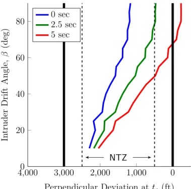
Figure 2-6 displays the intruder’s perpendicular deviation from the runway at the corresponding tc from Figure 2-5, with varying pilot response delays, for 3000 ft runway separation. Again, the lack of smoothness in the plot lines is due to the same discretization as in Figure 2-5. Notice that pilot response delay has a larger effect on tc, and thus the perpendicular distance from the nominal flight path at tc, as the intruder’s drift angle increases.
Figure 2-6 allows for comparison to a PRM approach, in which the controller would issue breakout instructions after the intruder violates a 2000 ft wide NTZ. This 2000 ft wide NTZ would begin 500 ft from the intruder’s nominal flight path when considering the 3000 ft runway separation of Figure 2-6. Considering the 5 s pilot response delay curve in Figure 2-6, the collision avoidance system would be able to effectively alert later than during PRM for intruder drift angles below 50° (where the curve crosses the 500 ft mark).
0 1,000 2,000 3,000 4,0000 20 40 60 80 NTZ Perpendicular Deviation at tc (ft) In truder Drift Angle, β (deg) 0 sec 2.5 sec 5 sec
Figure 2-6: Drift angle vs. perpendicular deviation
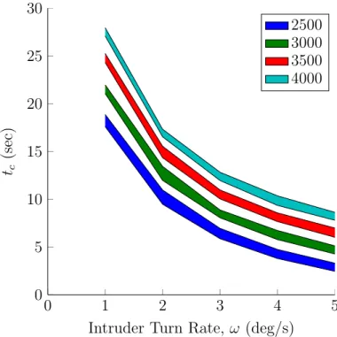
For a constant-turn blunder, the minimum (worst-case) available time to alert (tc) is calculated for a given runway separation and intruder turn rate ω, between 1 and 5 deg/s in 1 deg/s intervals, over all possible combinations of velocity, longitudi-nal runway stagger, and longitudilongitudi-nal aircraft stagger. The velocity for each aircraft is searched between 110 and 170 kt in 10 kt increments. Longitudinal runway and aircraft stagger are both searched between =4000 and 4000 ft in 400 ft increments. These larger increments, compared to those of the constant-drift analysis, are due to computational limitations.
Figure 2-7 displays the worst-case available time to alert (tc) versus turn rate ω for a 5 s pilot response delay and runway separations of 2500, 3000, 3500, and 4000 ft. The filled plot areas represent the tc range for avoidance maneuever vertical rates between 1500 and 2500 ft/min. For a given runway separation and intruder turn rate, an increased avoidance vertical rate from 1500 ft/min to 2500 ft/min only adds, at most, about 1 s to the available alert time tc. Since no curve passes below the tc = 0 line, there are no worst-case scenarios which absolutely preclude NMAC resolution. For 3000 ft runway separation, the worst-case available time to alert drops below 10 s
at intruder turn rates greater than or equal to 3 deg/s. Furthermore, each additional 500 ft of runway separation allows for approximately 2 s of additional time to alert.
0 1 2 3 4 5 0 5 10 15 20 25 30
Intruder Turn Rate, ω (deg/s) tc (sec) 2500 3000 3500 4000
Figure 2-7: Worst-case available time to alert (tc) vs. turn rate
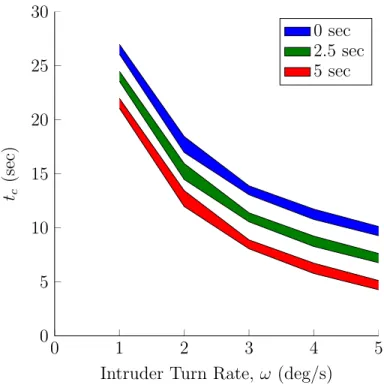
Figure 2-8 displays the worst-case available time to alert (tc) versus turn rate ω for 3000 ft runway separation and pilot response delays of 0, 2.5, and 5 s. The trends are similar to those observed in Figure 2-7. As expected, each additional 2.5 s of pilot response delay decreases the available time to alert by 2–3 s.
Figure 2-9 displays the intruder’s perpendicular deviation from the runway at the corresponding tc from Figure 2-8, with varying pilot response delays, for 3000 ft runway separation and a 2500 ft/min avoidance maneuever. Comparing the 5 s pilot response delay curve in Figure 2-9 with a PRM approach, the collision avoidance system would be able to effectively alert later than when using PRM for intruder turn rates less than 4 deg/s. With a standard 2000 ft NTZ and 3000 ft runway separation, PRM alerts when the intruder deviates 500 ft from centerline. Smaller pilot response delays allow for even greater advantages over PRM alert thresholds, as any intruder turn rate up to at least 5 deg/s does not require an RA until after the 500 ft mark.
0 1 2 3 4 5 0 5 10 15 20 25 30
Intruder Turn Rate, ω (deg/s) tc
(sec)
0 sec 2.5 sec 5 sec
Figure 2-8: Worst-case available time to alert (tc) vs. turn rate
0 1,000 2,000 3,000 4,0000 1 2 3 4 5 NTZ Perpendicular Deviation at tc (ft) In truder T urn Rate, ω (deg/s) 0 sec 2.5 sec 5 sec
2.3
Discussion
According to Figures 2-5 and 2-6, for reasonable blunders (around 30° drift angle or 3 deg/s turn rate) and assuming a 5 s pilot response delay and 3000 ft runway separation, the worst-case scenarios allow 5–10 s to alert after the blunder is initiated. These worst-case alerting requirements correspond to path deviations equal to or greater than those that would trigger a controller-issued alert during PRM operations, as displayed in Figures 2-6 and 2-9. There are no cases in which it is too late to avoid an NMAC (tc < 0) for any turn rate or any drift angle less than 70° at 3000 ft runway separations. However, Figure 2-6 reveals that there are some high-angle drift scenarios at 3000 ft runway separation that require an alert within only a few seconds of the start of a blunder.
Taking these conclusions into consideration, it is feasible that ACAS Xo can be tuned to meet the alerting criteria for all reasonable blunders and potentially more severe constant-turn blunders. Even in the worst-case and with the most conservative pilot response assumption (5 s), ACAS Xo could likely detect the blunder and alert in time to resolve any conflicts. Furthermore, in the case of the more severe drift blunders, even with a few seconds of available alert time, the blunder may be obvious enough from the outset that ACAS Xo is able to alert in time. The true abilities of ACAS Xo, however, cannot be realized until it is tuned for CSPO through surrogate modeling and automated search. This optimization process is described in the next chapter.
Chapter 3
Optimization via Surrogate
Modeling
To achieve optimal ACAS Xo performance with respect to a set of CSPO encounters, optimization via surrogate modeling is used to tune applicable design parameters. Optimization via surrogate modeling is an approach that aims to reduce computation time and increase optimization effectiveness in a large design space by testing data points that are most likely to lead to the global optimum. The goal of this study is to tune ACAS Xo for optimal performance during CSPO with respect to both safety and alerting behavior. The logic can be tuned by altering the settings of multiple design parameters, the effects and interactions of which are difficult to infer by human judgment.
The automated tuning procedure applied here begins with a screening study of a large initial set of design parameters to reduce the dimensionality of the search to a smaller subset of parameters. Latin hypercubes are optimized to generate a sampling plan that effectively samples the design space [15]. Each design parameter setting in the sampling plan is evaluated on 100,000 CSPO encounters using Monte Carlo simulation. Using the resulting sample data, a surrogate model is generated that estimates the model parameters, and thus the performance function (the “black-box” function) at each point in the design space. The sample data and surrogate model are updated after testing each new infill point (additional sample point) that meets
the Maximum Expected Improvement criterion. With sufficient data, this iterative process converges on the optimum [11]. Figure 3-1 outlines the process.
Initial Parameters Screened Parameters Initial Sample Data Estimated Model Parameters Updated Sample Data New Infill Point Screening Sampling plan and simulation Generate model Regenerate model
Search for Max Expected Improvement Simulate point
Figure 3-1: Overview of the optimization via surrogate modeling process
3.1
Performance Metrics
As previously stated, the ultimate goal is to tune ACAS Xo for optimal safety and alerting behavior during CSPO. Safety and alerting behavior can generally be mea-sured by two performance metrics:
Risk Ratio = NMACs with collision avoidance
NMACs without collision avoidance, (3.1)
Nuisance Alert Rate = Alerts in non-NMAC encounters
Non-NMAC encounters . (3.2)
The output of the Monte Carlo simulations includes information about each en-counter, such as whether an NMAC occurs and whether an RA is issued. The CSPO encounters are also simulated without any collision avoidance system to determine
which encounters nominally result in an NMAC. An NMAC is defined to occur when two aircraft come within 500 ft horizontally and 100 ft vertically of each other.
Additional performance metrics not involved in the optimization process may still be of interest when analyzing collision avoidance system performance. These addi-tional metrics, referred to as secondary metrics, relate to specific behaviors during an RA, such as strengthenings and reversals. For example, a Climb (1500 ft/min) command could be strengthened to a 2500 ft/min climb rate or reversed to a De-scend command (1500 ft/min). Though strengthenings and reversals are sometimes necessary, they should be minimized when possible due to their disruptive nature [21]. Table 3.1 lists the performance metrics considered in this study. The metrics in boldface correspond to the primary metrics of Equations 3.1 and 3.2 that are used in the tuning process. The performance metrics of Table 3.1 are also commonly used for ACAS Xa performance assessments.
Table 3.1: Optimization Performance Metrics
Metric Description
Unresolved NMACs # NMACs that occur when an alert is issued and when an NMAC would have occurred otherwise
Induced NMACs # NMACs that occur when an alert is issued but when an NMAC would not have occurred otherwise
Missed Alerts # NMACs that occur when no alert is issued
Risk Ratio Ratio of total NMACs with collision avoidance to NMACs without collision avoidance
Nuisance Alert Rate Rate of alerting in encounters where no NMAC occurs both with and without collision avoidance
Strengthenings # encounters that include a strengthening command Reversals # encounters that include a reversal command
3.2
Historical Encounter Set
To support the tuning efforts described in this thesis, an historical CSPO encounter set of 100,000 encounters was generated to enable Monte Carlo simulation. A tech-nical report describes the historical CSPO encounter model development in further detail [41]. Individual encounters are used to simulate certain aircraft dynamics,
con-figurations, and procedures by specifying the states of multiple aircraft at regular time intervals. This encounter set includes significant aircraft blunders and is used to assess system safety as well as alerting behavior.
For every encounter, runways are separated by 3000 ft without stagger. A runway separation of 3000 ft is selected because it represents the minimum distance allowed for parallel operations without addressing the risk of wake turbulence. For each encounter, two aircraft are initialized so that they come within 2000 ft of each other’s longitudinal position at some point along the approach path.
Figure 3-2: Example encounter generation
The 100,000 encounters are generated by randomly selecting two aircraft tracks from an historical trajectory library. The library contains approximately 140,000 tracks of aircraft on approach to landing during IMC at various airports in the NAS. Three main assumptions were required to create the historical trajectory library [41]:
Only including trajectories from IMC periods results in only instrument ap-proach trajectories.
Lateral deviations about the localizer are symmetrically distributed.
An approach path’s glide slope is best determined by the mode of the discretized probability distribution.
Each aircraft track is transformed (rotated and/or flipped) such that the aircraft approaches a generic runway 09L or 09R (east-bound). To create an encounter, two trajectories are transformed to approach the desired parallel runways. An illustration of this process is provided in Figure 3-2.
Each sampled trajectory begins at least 10 NM from the runway threshold. The sampling process biases trajectories with large deviations over small deviations by up to a factor of 1000. Nominally, each pair of trajectories should be vertically separated by at least 1000 ft when entering the localizer beam, which guides each aircraft’s lateral position. Blunder types include incorrect altitude join-ups, incorrect ILS captures (Figure 3-3(a)), and break-out maneuvers in the direction of the paired aircraft (Figure 3-3(b)), each occurring at a rate of one per hundred approaches. This rate is chosen so that ACAS Xo is tested against a sufficiently high number of severe blunders.
(a) Incorrect ILS capture (b) Break-out (c) Large-angle intercept
Figure 3-3: Example aircraft behavior
Because the aircraft trajectories are sampled directly from the historical library, they exhibit a wide range of behavior, including intercepting the localizer at large angles (Figure 3-3(c)) and capturing the ILS at a variety of altitudes and distances from the runway. Some of these behaviors are outside those observed during actual CSPO operations in IMC. The goal of such an encounter set is to allow for simulations over a wide range of possible scenarios. This is the encounter set that is used to tune ACAS Xo for CSPO.
3.3
Simulation and Evaluation
Collision avoidance system performance is evaluated on a given encounter using Monte Carlo simulation. Both TCAS and ACAS Xo aircraft are simulated to be equipped with the same surveillance capabilities to determine the range, bearing, and altitude of other aircraft within radar range. The range and bearing measurements are corrupted with zero-mean Gaussian noise with 50 ft and 10° standard deviations, respectively, to account for surveillance uncertainty, while the altitude is quantized to 25 ft.
The state space within which the sensor measurements are taken must be dis-cretized so that the ACAS X solution is computationally feasible to obtain. Variables within the horizontal and vertical dimensions are discretized such that the state space is adequately defined. A pilot response model must also be defined to accurately reflect pilot response delays observed in real life. For both TCAS and ACAS X sim-ulations, the pilot response model includes a 5 s initial pilot response delay and a 3 s subsequent pilot response delay. In other words, the pilot will begin to respond 5 s after an initial RA is issued and 3 s after any additional RAs are issued.
After an encounter is simulated, a wide variety of performance metrics can be extracted for that encounter. For the purposes of tuning ACAS Xo, these metrics include:
Whether an RA is issued for either aircraft
Whether a strengthening RA is issued for either aircraft Whether a reversal RA is issued for either aircraft Whether the encounter results in an NMAC
A set of encounters can be simulated with any combination of unequipped aircraft (i.e., lacking a collision avoidance system) and aircraft equipped with TCAS or ACAS Xo. By simulating an encounter set with two unequipped aircraft, in ad-dition to simulating with equipped aircraft, the performance metrics for each case can be combined to output additional meaningful metrics for each encounter, such
as specific NMAC types. For example, an NMAC resulting from a simulation of equipped aircraft is categorized as an induced NMAC if the unequipped simulation of the same encounter does not result in an NMAC. Unresolved NMACs and missed alerts can be similarly extracted from the raw output metrics.
3.4
Defining the Objective Value
The collision avoidance system performance for a given set of encounters is essentially a “black-box” function since the performance cannot be known until simulations are performed for each combination of design parameter settings. An underlying premise of surrogate modeling is that the performance of the system can be defined by a single function value, or objective value, at each point in the design space. Based on the objective values at different parameter settings, a surrogate model for the function can be estimated with increasing accuracy as more data points are intelligently selected and tested over time to find the “black-box” function’s global optimum.
Utility elicitation is one concept that helps generate an objective function which combines performance metrics into a single objective value [38]. Examples of utility elicitation methods include additive modeling, swing weight elicitation, and rank-weighting [8]. Although several methods are available to elicit preferences from users to determine the appropriate attribute rankings and relative weightings, utility elici-tation is not within the scope of this study.
The objective function is formulated as a linear combination of two performance metrics: risk ratio and nuisance alert rate. A weighting sweep is performed to test various linear combinations of performance metrics and select the weighting that most effectively tunes ACAS Xo. The weighting sweep procedure and results are provided in more detail in Appendix A. Since safety is the primary concern, the risk ratio is given more weight than the nuisance alert rate, resulting in the following objective function:
Risk ratio also requires more weight due to its lower-magnitude values compared to those of nuisance alert rate. The selected linear combination in Equation 3.3 is cross-referenced and confirmed with a subjective hand-ranking of data points with respect to overall performance. Such a simple linear combination of performance metrics has been shown to perform well in decision-making processes [5].
3.5
Screening Study
To maximize computational efficiency in the optimization process, the scope of the tuning process is reduced. For the ACAS Xo problem, the scope correlates to the number of design variables that will be tuned. The ACAS X logic incorporates 46 distinct design parameters. Based on prior knowledge of ACAS X, the eight param-eters listed in Table 3.2 were deemed appropriate to tune and potentially relevant to ACAS Xo behavior in CSPO encounters. These parameters are discussed in further detail in technical reports [1, 21]. The goal of the screening study is to extract the most significant parameters affecting the performance metrics of interest, specifically the primary metrics of risk ratio and nuisance alert rate.
Table 3.2: Design Parameters Analyzed in the Screening Study
Parameter Description
r alert Cost of issuing an RA to the pilot
r maintain < 1500 ft/min Cost of issuing a “Maintain Vertical Rate” command when the current vertical rate is < 1500 ft/min
ddx ddy sigma Intruder horizontal acceleration deviation
cycles Number of seconds for which alerting is allowed when in horizontal conflict horiz. conflict def. Horizontal range that defines an NMAC for logic calculations
vert. conflict def. Vertical range that defines an NMAC for logic calculations
slow clos. rho thresh. Range threshold where time until conflict is calculated using horizontal and vertical information
slow clos. drho thresh. Range rate threshold where time until conflict is calculated using horizontal and vertical information
To determine the most significant parameters relative to each performance metric, the elementary effect on the primary and secondary performance metrics is calculated;
that is, a sensitivity study is performed. The elementary effect for each parameter-metric pair is expressed by a mean and standard deviation. The mean value measures the change in the performance metric for a given change in the parameter. A large-magnitude mean indicates that the parameter has a strong effect on the given metric. A large standard deviation indicates that the parameter experiences strong interac-tions with other parameters [11].
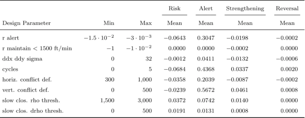
Table 3.3: Design Parameter Screening Study Results (Mean)
Risk Alert Strengthening Reversal
Design Parameter Min Max Mean Mean Mean Mean
r alert −1.5 · 10−2 −3 · 10−3 −0.0643 0.3047 −0.0198 −0.0002
r maintain < 1500 ft/min −1 −1 · 10−2 0.0000 0.0000 −0.0002 0.0000
ddx ddy sigma 0 32 −0.0012 0.0411 −0.0132 −0.0006
cycles 0 5 −0.0684 0.4368 0.0337 0.0020
horiz. conflict def. 300 1,000 −0.0358 0.2039 −0.0087 −0.0002
vert. conflict def. 0 500 −0.0239 0.5672 0.0461 0.0008
slow clos. rho thresh. 1,500 3,000 0.0372 0.0742 0.0140 0.0000
slow clos. drho thresh. 0 500 0.0191 0.0131 0.0008 0.0000
Table 3.4: Design Parameter Screening Study Results (Standard Deviation)
Risk Alert Strengthening Reversal
Design Parameter Min Max Std Dev Std Dev Std Dev Std Dev
r alert −1.5 · 10−2 −3 · 10−3 0.0556 0.1963 0.0174 0.0004
r maintain < 1500 ft/min −1 −1 · 10−2 0.0000 0.0000 0.0002 0.0000
ddx ddy sigma 0 32 0.0009 0.0409 0.0127 0.0009
cycles 0 5 0.0820 0.2817 0.0349 0.0019
horiz. conflict def. 300 1,000 0.0378 0.1434 0.0262 0.0010
vert. conflict def. 0 500 0.0349 0.3387 0.0356 0.0009
slow clos. rho thresh. 1,500 3,000 0.0540 0.1082 0.0270 0.0000
slow clos. drho thresh. 0 500 0.0314 0.0251 0.0017 0.0002
Table 3.3 shows the eight parameter ranges and the mean elementary effect for each parameter-metric pair. As an example, the cycles parameter, which was tested between values of 0 and 5, exhibits a relatively large-magnitude elementary effect for each of the four metrics. Therefore, the cycles parameter has a significant effect on each of the performance metrics and is included in the optimization process moving
forward. The standard deviations are also included in Table 3.4. The results indicate a strong correlation between design parameters with a large standard deviation and those with a large mean.
The five parameters that exhibit significant elementary effects for the primary metrics are: (1) cost of alerting, (2) number of cycles, (3) horizontal conflict definition, (4) vertical conflict definition, and (5) slow closure rho threshold. The cost of alerting relates to the cost of issuing an initial RA to the pilot. The cycles parameter indicates the number of seconds the logic may continue issuing an RA while the two aircraft remain in horizontal conflict for an extended period of time. The cycles parameter is particularly relevant when considering CSPO encounters in which low closure rates are prevalent. The horizontal and vertical conflict definitions define the NMAC region on which the ACAS X logic bases its calculations, though the actual horizontal and vertical NMAC definitions remain unchanged (500 ft and 100 ft, respectively) for the performance metrics. The slow closure rho threshold parameter defines the range threshold between aircraft where ACAS X begins using both horizontal and vertical state information to calculate the estimated time until conflict. These five design parameters are used for the remainder of the tuning of ACAS Xo for CSPO.
3.6
Sampling Plan
The next step to prepare for the optimization is to generate a sampling plan that will provide a uniform, space-filling initial data set over the design space. This initial sampling plan will lead to a well informed surrogate model from which additional infill points can be intelligently selected for testing. The sampling plan is generated using Latin hypercubes that are optimized with respect to the Morris-Mitchell cri-teria. The result is a sampling plan that does not repeat any one parameter setting and comprehensively samples the design space [11]. Forty sample points, each rep-resenting a combination of parameter settings, are tested on the historical encounter set of 100,000 CSPO encounters. Table 3.5 lists the ranges used for the five design parameters.
Table 3.5: Design Parameter Ranges used for Optimization
Design Parameter Min Max r alert −5 · 10−3 −2.5 · 10−3
cycles 4 7
horiz. conflict def. 200 400 vert. conflict def. 0 100 slow clos. rho thresh. 1,500 2,500
3.7
Surrogate Modeling
After simulating the 100,000 CSPO encounters from the historical encounter set, and calculating objective values using Equation 3.1 through Equation 3.3 for each parameter setting from the sampling plan, a surrogate model can be generated that approximates the objective value of Equation 3.3 at every point in the design space. The Kriging model is a Gaussian process based model that allows for the calcula-tion of a prediccalcula-tion mean and variance at every point in the design space. The Kriging model is chosen for its ability to model complex functions and measure uncertainty at each point [22]. Specifically, the Kriging model is defined by the radial basis function of the form ψ(i) = exp − k X j=1 θj|x (i) j − xj|pj . (3.4)
The Kriging basis function only differs from a Gaussian basis function in that the Kriging basis allows the width and smoothness of the function to vary in each di-mension. Holding the width and smoothness constant for every parameter yields the Gaussian basis function [11].
In Equation 3.4, ψ denotes the basis function (one centered at each data point), k is the number of design parameters (dimensionality), θ defines the basis function width (also known as the “activity” parameter) for each dimension, and p determines the function smoothness for each dimension. The sample data and their observed
responses (objective values) are defined, respectively, as follows:
X = {x(1), x(2), ..., x(n)}T, (3.5)
y = {y(1), y(2), ..., y(n)}T. (3.6)
The observed responses at each data point are considered to be derived from a stochas-tic process with mean 1µ, where 1 is an n by 1 vector of ones:
Y = {Y (x(1)), ..., Y (x(n))}T. (3.7)
The basis function of Equation 3.4 can then be used to calculate the correlation between each pair of responses, resulting in an n by n correlation matrix Ψ, where an element Ψ(i, l) of the matrix is defined by
cor[Y (x(i)), ..., Y (x(l))] = exp
− k X j=1 θj|x (i) j − x (l) j |pj . (3.8)
The correlation between a pair of responses, expressed by Equation 3.8, depends on the distance between each point as well as the θ and p parameters [11].
The next step in generating the surrogate model is to calculate maximum likeli-hood estimates (MLEs) for the parameters µ and σ, which are base terms used to define the model. The MLEs of µ and σ are calculated by maximizing the likelihood of the existing sample data given the parameters:
L(Y(i), ..., Y(n)|µ, σ) = 1 (2πσ2)n/2 exp " − Pn i=1(Y (i)− µ)2 2σ2 # . (3.9)
Equation 3.9 can be expressed in terms of its natural logarithm and the existing data set: ln(L) = n 2ln(2π) − n 2ln(σ 2) − 1 2ln |Ψ| − (y − 1µ)TΨ−1 (y − 1µ) 2σ2 . (3.10)
By setting the derivatives of Equation 3.10 to zero, the MLEs for µ and σ2 can be extracted [11]: ˆ µ = 1 TΨ−1 y 1TΨ−1 1, (3.11) ˆ σ2 = (y − 1µ) TΨ−1 (y − 1µ) n . (3.12)
These MLEs can be substituted back into Equation 3.10 to derive the concentrated log-likelihood function (constant terms removed) which depends on θ and p via Ψ [11]:
ln(L) ≈ −n 2 ln(ˆσ
2) − 1
2ln |Ψ|. (3.13)
The log-likelihood function in Equation 3.13 is not differentiable and requires numer-ical optimization to maximize the function and find MLEs for θ and p.
A genetic algorithm was applied throughout this process [12, 42]. The parameter θ was searched on a logarithmic scale from 10−3 to 103, and p was searched from 1 to 2. After finding the MLEs for each model parameter, a prediction can be made at any point in the design space by maximizing the conditional likelihood of the existing data set and the point’s predicted objective value. After defining a vector ψ of correlations between the prediction point and each existing observed value, the objective value prediction at a point x in the design space can be calculated [11] by
ˆ
y(x) = ˆµ + ψTΨ−1(y − 1ˆµ). (3.14)
3.8
Searching the Model
After developing the Kriging model to estimate the objective value at each point in the design space, a search algorithm must determine which point in the design space, known as an infill point, to test next and efficiently drive toward the optimum design setting with the best performance. This determination relies on a specific heuristic to be used in computing the expected reward of sampling a certain point. In searching for the global optimum, an heuristic can be designed to focus on global exploration,

![Figure 1-3: Aircraft trajectories and TCAS commands in the ¨ Uberlingen mid-air collision [23]](https://thumb-eu.123doks.com/thumbv2/123doknet/14370143.504221/13.918.154.777.708.924/figure-aircraft-trajectories-tcas-commands-uberlingen-mid-collision.webp)