en fr

HAL Id: tel-01228505

https://tel.archives-ouvertes.fr/tel-01228505

HAL is a multi-disciplinary open access archive for the deposit and dissemination of sci-entific research documents, whether they are

pub-L’archive ouverte pluridisciplinaire HAL, est destinée au dépôt et à la diffusion de documents scientifiques de niveau recherche, publiés ou non,

to infections

Eugenio Valdano

To cite this version:

Eugenio Valdano. Computing the vulnerability of time-evolving networks to infections. Santé publique et épidémiologie. Université Pierre et Marie Curie - Paris VI, 2015. English. �NNT : 2015PA066211�. �tel-01228505�

THESE DE DOCTORAT DE L’UNIVERSITE PIERRE ET MARIE CURIE

Spécialité Biomathématiques

École Doctorale Pierre Louis de Santé Publique à Paris : Épidémiologie et Sciences de l’Information Biomédicale

Présentée par M. Eugenio VALDANO

Pour obtenir le grade de

DOCTEUR de l’UNIVERSITÉ PIERRE ET MARIE CURIE

Analyse quantitative de la vulnérabilité

des réseaux temporels aux maladies infectieuses

à soutenir le 13 octobre 2015 devant le jury composé de :

M. le Docteur Alain BARRAT (CNRS Marseille) Examinateur

Mlle le Docteur Vittoria COLIZZA (Université Pierre et Marie Curie) Co-directrice de thèse M. le Docteur Philipp HÖVEL (Technische Universität Berlin) Rapporteur

Mme le Professeur Clémence MAGNIEN (Université Pierre et Marie Curie) Examinateur M. le Professeur Guy THOMAS (Université Pierre et Marie Curie) Directeur de thèse Mme le Docteur Elisabeta VERGU (INRA) Rapporteur

Résumé de la thèse

Résumé de la thèse

Introduction

Les modèles mathématiques représentent une contribution importante dans la lutte contre les maladies infectieuses, comme ils représentent un outil pour définir des stra-tégies pour réduire le nombre de cas, utiliser de façon optimale des ressources limitées, faire face rapidement aux émergences, et mettre en place des mesures d’endiguement efficaces. Depuis leur introduction, ces modèles, qu’on appelle modèles à compartiments, sont basés sur la supposition que l’évolution et la transmission de la maladie puissent être traduites en un ensemble de règles simples et qui peuvent être adaptées à des agents pathogènes caractérisés par différents pathophysiologie, développement clinique, et étio-logie (virus, bactéries, etc.). L’épidémie est donc interprétée comme un comportement émergent de l’interaction parmi les hôtes [1–5]. Néanmoins, dans le passé, l’utilisation de modèles mathématiques en santé publique a été limitée par le manque de données sur les interactions humaines. Récemment, la situation a radicalement changé, grâce à l’avènement de la science des données, grâce à laquelle il est devenu possible d’enregis-trer de façon très précise les contacts et les transports responsables de la propagation des maladies. Actuellement, on a des bases de données qui décrivent l’interaction entre personnes, dans différents contextes et à différentes échelles : des contacts sociaux à la mobilité, jusqu’aux contacts sexuels [6–34]. En outre, les activités humaines ne sont pas le seul objet de recherche : il est maintenant possible de suivre les mouvements d’animaux de ferme [35–40], afin d’étudier la propagation des nombreuses maladies qui menacent la santé des animaux, l’économie, et finalement même la santé humaine.

Épidémies et réseaux

Afin de gérer ces structures des contacts complexes, de nouveaux outils théoriques ont été adapté et développé, qui considèrent la propagation de maladies comme un processus dynamique sur réseaux [41–48]. Les réseaux sont en fait devenus un outil essentiel qui, en représentant les populations en tant de nœuds (hôtes potentiels de l’agent pathogène) et des liens (interactions entre hôtes), permettent d’appliquer au contexte des maladies in-fectieuses le formalisme de la physique statistique, la théorie des graphes, et des systèmes dynamiques.

La dynamique épidémique sur réseau suppose que chaque nœud peut se trouver dans une des stades de la maladie prédites par le modèle à compartiments de référence, et que le processus de l’infection se déroule par les liens : chaque nœud a une probabilité d’infecter (transmissibilité) un nœud susceptible auquel il est connecté.

Un aspect clé dans la modélisation épidémique concerne l’émergence du régime épidé-mique. Quand un agent pathogène est introduit dans une population susceptible, deux scénarios sont possibles : soit le nombre d’infectés va vite à zéro, en conduisant rapide-ment à l’extinction, soit il augrapide-mente de façon exponentielle, ce qui entraîne une flambée

épidémique. Être capable de prédire lequel des deux aura lieu est fondamental pour es-timer la vulnérabilité de la population attaquée par un agent pathogène spécifique, et ensuite pour évaluer les stratégies les plus efficaces d’immunisation. Ce concept de vul-nérabilité de la population est formalisé en termes de seuil épidémique [4, 41], qui est la valeur critique de la transmissibilité qui distingue extinction et régime épidémique. L’épi-démiologie computationnelle a fourni des outils pour calculer analytiquement la valeur du seuil épidémique pour de nombreux modèles épidémiques, et pour de différents types de structures de contact. En particulier, grâce à l’intégration de la théorie des réseaux, il a été possible d’évaluer l’impact des différentes caractéristiques topologiques sur la vul-nérabilité, comme la présence de nœuds avec un degré (nombre de contacts) exception-nellement élevé, qu’on appelle hubs. Il a été montré, en effet, que leur présence augmente considérablement la vulnérabilité du réseau, en réduisant le seuil épidémique. Pour mon-trer cela analytiquement, on va supposer un modèle susceptible-infecté-susceptible (SIS), dans lequel les nœuds infectés transmettent la maladie aux voisins susceptibles avec une probabilité , et qui guérissent avec une probabilité µ. Ce modèle est clairement une simplification du développement clinique réel d’une maladie ; il représente néanmoins un modèle utile et applicable à des maladies qui admettent l’existence d’un état endémique, comme un grand nombre d’infections bactériennes. On suppose en outre que P (k) soit la distribution des degrés du réseau. Le seuil épidémique ( c) peut donc s’exprimer en

termes des moments de cette distribution [41, 49, 50] : c = µ_hkhki2_i;vu que la présence de

hubs induit de fortes variations de degré, le second moment de la distribution est très grand. Cela signifie que le seuil est très bas, et diminue de plus en plus avec l’augmen-tation de la taille de la population. Le valeur du seuil dans ce type d’approche découle des propriétés statistiques des classes de réseaux (annealed) ; il est également possible de prendre en compte la topologie explicite du réseau de contacts à travers le forma-lisme de la matrice d’adjacence (quenched). En supposant un réseau de N nœuds, indicés i, j = 1,· · · , N, on définit la matrice d’adjacence [51] A, de taille N ⇥ N, et d’éléments Aij = 1 si i est connecté à j, et Aij = 0 autrement. Le seuil épidémique peut ansi être

calculé en termes du spectre de la matrice d’adjacence [52, 53] :

c = µ

⇢[A], (1)

où ⇢[A] est le rayon spectral de la matrice d’adjacence, soit le maximum parmi les valeurs absolues de ses valeurs propres.

Seuil épidémique sur des réseaux temporels

Les résultats décrits ci-dessus ont été développées en supposant que les maladies se pro-pagent sur des réseaux qui ne varient pas dans le temps, ou qu’ils le fassent à des échelles de temps très différentes de celles de la diffusion de l’agent pathogène. Dans de différents contextes, il a cependant été observé que les contacts et l’épidémie évoluent sur des temps caractéristiques comparables ; il a également été montré que l’interaction entre l’évolution du réseau et le processus de l’infection influence sensiblement le résultat du processus

Résumé de la thèse épidémique [13, 54–59], les conditions de déclenchement, de persistance et d’endémicité. Par conséquent, une méthodologie qui aspire à une évaluation quantitative du risque doit tenir compte de l’évolution temporelle de contacts. Le formalisme des réseaux temporels (ou réseaux dynamiques) [60–62], où le réseau lui-même devient un processus dynamique qui détermine l’évolution des liens, peut être utilisé efficacement pour représenter ce type de structure ; cependant, il a été noté que les propriétés émergentes de ces nouveaux systèmes sont conceptuellement et phénoménologiquement nouvelles, et ne peuvent gé-néralement pas être considérées comme de simples extensions de ce qui est connu pour les réseaux statiques. En particulier, l’étude du seuil épidémique a été limiteé à des ap-proches numériques ou des apap-proches analytiques pour des cas spécifiques [59, 63–67]. Dans cette thèse, nous proposons une nouvelle méthode, publiée dans [68, 69], pour cal-culer analytiquement le seuil épidémique pour un réseau temporel générique. Le concept fondamental derrière cette méthode est de représenter le réseau en termes d’un objet sta-tique : le réseau multi-couches (ou multi-layer) [70, 71]. Dans ce type d’objet les nœuds sont divisées en plusieurs couches, et les liens qui joignent des nœuds de la même couche ou de couches différentes sont interprétées de manière différente. On propose une façon innovatrice pour représenter le réseau temporel, où chaque pas de temps est représenté comme une couche qui contient une copie de tous les nœuds du réseau, et les liens du réseau temporel se traduisent en termes de liens entre les couches du réseau multi-couche. Les règles de construction du réseau multi-couche sont illustrées dans la Figure R1. La structure spécifique de cette projection permet de prendre en compte aussi la dynamique de l’infection. Le résultat est un objet qui représente à la fois le processus dynamique de l’évolution structurelle des contacts, et le processus de propagation de l’épidémie. Cet aspect nous a permis de résoudre analytiquement le calcul du seuil épidémique ; en particulier, on montre qu’il peut être dérivé à partir de ce que nous appelons propaga-teur d’infection [69]. En supposant un réseau temporel de T pas de temps, chacun avec matrice une d’adjacence At, le propagateur d’infection a la forme suivante :

P =

T

Y

t=1

(1 µ + At) . (2)

On montre que le seuil épidémique est la valeur minimale de transmissibilité c pour

laquelle ⇢[P ( c, µ)] = 1 [72]. Le propagateur d’infection représente en fait le potentiel

de propagation, puisque l’élément Pij est égale à la probabilité que le nœud i, infectieux

au temps t = 1, donne lieu à un nœud j qui soit infectieux au temps t = T , dans l’approximation quenched mean field [52, 53, 73] avec laquelle on l’a calculé.

En [68] on n’a introduit cette méthode que pour le modèle de diffusion SIS ; dans [69] on montre que la forme du propagateur d’infection décrite dans l’Equation 2 est valable même pour des maladies qui confèrent l’immunité après la guérison, soit temporaire soit permanente. La précision de notre mesure du seuil peut être estimée avec des simulations numériques de l’infection, en mesurant la fraction de nœuds infectés en fonction de la transmissibilité, lorsque la maladie atteint l’état endémique : la Figure R2A montre un exemple de cette approche.

t temporalt+1 multilayer

node i existing at times t,t+1 (i,t) (i,t+1)

(i,t) (j,t+1) (j,t) (i,t+1) (i,t) (j,t)

contacts

Figure R1: Représentation multi-couche du réseau temporel. Ici sont décrites les règles pour construire notre représentation multi-couches du réseau temporel, en uti-lisant seulement trois nœuds et deux pas de temps. Les liens qui joignent des représentations du même nœud sont pondérées avec 1 µ, afin de représenter le processus de guérison – plus précisément de non-guérison – en termes de transmission de la maladie à soi-même dans le futur ; par contre, les liens qui re-présentent les contacts du réseau temporel sont pondérés avec la transmissibilité

Résumé de la thèse 0 0.01 0.02 0.03 0 0.004 0.008 0.012 λc λc T (10mins) 18 12 6 1 24 30 36 9 55.7 11am 1pm 3pm B 0.08 0.06 0.04 λ 0.02 0 0.1 ‹i› 1 A 0.8 0.6 0.4 0.2 1 0 μ=0.2 μ=0.5

Figure R2: Validation du calcul du seuil, et influence du temps total du réseau sur le seuil. On considère ici un réseau de contacts sociaux dans un lycée, enregistré par Salathé et collaborateurs [7]. EnA on montre la fraction des nœuds infectés à l’équilibre (état endémique) en fonction de la transmissibilité, pour deux valeurs de probabilité de guérison (en rouge et bleu). Les flèches montrent la valeur théorique du seuil, calculée avec le propagateur d’infection. Les croix (MC) ont été obtenues de la solution numérique du processus de Markov (Equation 2 dans [68]), tandis que les points gris représentent le résultat des simulations microscopiques, dans lesquelles chaque nœud infectieux peut contaminer les nœuds sains avec lesquels il est en contact (ses voisins). En B on montre la valeur du seuil épidémique c(T )obtenu en considérant que le premiers T pas

de temps. L’histogramme en gris est en échelle linéaire et montre le degré moyen associé au pas de temps T .

contact empiriques registrent seulement une partie limitée dans le temps des interactions, il est important d’évaluer l’impact d’une telle longueur temporelle sur l’estimation du seuil, et par conséquent notre capacité à évaluer la vulnérabilité du système . En [68] on explore cet aspect, en essayant d’identifier la période de prise de donnée minimale qui soit optimale pour caractériser le propagateur d’infection ; on en montre un exemple en Figure R2B.

En plus de la durée totale de la prise de données, le calcul du seuil permet d’éva-luer l’impact d’autres caractéristiques des prises des données empiriques, y compris la résolution temporelle, que nous analysons dans [69].

La représentation multi-couches du réseau temporel, qui est le cœur de notre métho-dologie de calcul du seuil, n’est possible que si on suppose que l’évolution du réseau se déroule en temps discret, ce qui représente une limite lorsque nous traitons des systèmes pour lesquels le temps est un paramètre continu. Pour résoudre ce problème, on montre que la limite continue du propagateur d’infection est obtenue en résolvant un système différentiel qui contient la matrice d’adjacence A(t) du réseau temporel :

d

dtP (t) = P (t) [ m + lA(t)] , (3)

où l, m sont les taux de transmission et de guérison de la maladie. Une fois qu’on a trouvé le propagateur d’infection, le seuil peut être calculé avec son rayon spectral, comme dans le cas discret.

Les modèles épidémiques dont nous avons parlé jusqu’à maintenant ne prennent pas en compte une caractéristique commune à nombreuses maladies : la période de latence, c’est-à-dire le temps qui passe entre être infecté et devenir infectieux. Dans le cas des réseaux statiques la latence n’a pas d’impact sur le seuil épidémique [50], par contre cela n’est plus vrai pour les réseaux temporels, en raison de l’interaction entre les trois échelles de temps en jeu : évolution du réseau, durée d’infection, et période de latence. Le modèle SIS peut être modifié pour prendre en compte ce nouvel ingrédient, en devenant susceptible-exposé-infectieux-sensible (SEIS). La progression de la maladie est similaire au cas du SIS, sauf que les individus infectées ne sont pas immédiatement infectieux (E) ; ils deviennent infectieux avec une probabilité ✏ à chaque pas de temps.

Notre objectif est de calculer le propagateur d’infection du modèle SEIS sur réseaux temporels, et pour ce faire, nous utilisons à nouveau le formalisme des réseaux multi-couches. En particulier, on part du cas statique, et on démontre que le modèle SEIS sur un réseau A générique a le même seuil d’un modèle SIS sur un réseau à 2 couches. La structure spécifique du réseau 2-couches et les paramètres du modèle SIS permettant cette analogie sont décrits dans la Figure R3. Une fois démontré cette équivalence, la généralisation au cas temporel est obtenue en appliquant les résultats précédents [68,69]. On obtient ansi le propagateur d’infection ˆP pour le modèle SEIS, en termes de matrices composées de quatre blocs N ⇥ N :

ˆ P = T Y t=1 ✓ 1 µ ✏ At 1 ✏ ◆ (4)

Résumé de la thèse

A B

Figure R3: Représentation de la structure à deux couches pour le calcul du seuil épidémique en incluant la latence. A représente le réseau statique initial. B représente la projection multi-couches. Chaque nœud a une copie sur chaque couche, et la copie dans la couche 2 est connectée à la copie dans la couche 1 avec un lien direct (flèches noires pointillées). Chaque lien présent enA se traduit par deux liens directs de la couche 1 à la couche 2 (flèches rouges pointillées). À cette structure on couple un processus SIS, dans lequel les liens noirs ont une probabilité de transmission égale à ✏, tandis que les rouges . De plus, la probabilité de guérison dans la couche 1 est µ, et dans la couche 2 est ✏.

Réseaux de déplacements des bovins

Les maladies des animaux de ferme ont une grande pertinence dans le contexte de la santé publique, car elles menacent la santé et le bien-être animal, et ont un effet négatif sur l’économie, en termes de réduction de la productivité et de coûts de l’éradication [74,75]. De plus, elles représentent un danger direct pour la santé humaine [76].

En raison de sa position géographique et son marché de bétail intégré, l’Europe est constamment menacée par divers agents pathogènes, y compris la fièvre aphteuse [74,77, 78], la diarrhée virale bovine [79–81], la tuberculose bovine [82–84] et la brucellose [85–87] pour les bovins, la fièvre catarrhale du mouton pour tous les ruminants, la peste porcine classique [88] et africaine [89] pour les porcs. Bien que ces maladies ont des caractéris-tiques épidémiologiques très différentes les unes des autres, elles se propagent toutes, exclusivement ou en partie, grâce aux mouvements d’animaux entre les structures ; pour cette raison, l’étude des réseaux de mouvements est extrêmement importante. De nom-breuses études ont déjà été publiées, sur des pays et espèces différents. Dans cette thèse, nous nous concentrons sur le marché des bovins, et développons une analyse compa-rative des mouvements dans trois pays européens : l’Italie, la Suède, la Hongrie, grâce à la coopération avec les institutions compétentes1_{. La Figure R4 montre la définition}

des réseaux, et leur représentation agrégée. Ces réseaux sont intrinsèquement temporels, parce que les mouvements sont enregistrés quotidiennement.

Nous avons observé que ces réseaux montrent une phénoménologie extrêmement riche et diversifiée en termes de propriétés globales, temporelles, et géographiques. En par-1. Istituto Zooprofilattico Sperimentale “G. Caporale” (Italie), Linköping University (Suède), Hunga-rian National Food Chain Safety Office (Hongrie).

A w<10 IT A HUN SWE w≥10 B C D E F

Figure R4: Réseau bovin agrégé. Représentation du réseau des mouvements des bovins, agrégé sur une période d’un an : 2008 pour l’Italie (A,B) et la Suède (E,F), 2010 pour l’Hongrie (C,D). Les nœuds (les structures qui participent au marché) sont placés en fonction de leur position géographique ; les lien représentent les déplacements de bovins d’un nœud à l’autre, composés de moins (A,C,E) ou plus de 10 animaux (B,D,F).

Résumé de la thèse ticulier, les réseaux agrégés à échelles de temps différentes présentent des topologies hétérogènes dans les trois pays. En outre, l’échelle de temps qui domine l’évolution de chaque réseau est la semaine ; par contre les effets saisonniers tendent à être spécifiques à chaque pays. Les caractères spatiaux aussi ont tendance à varier d’un pays à l’autre, car ils répondent à la diversité climatique et géographique.

Analyse du risque

Le calcul du seuil épidémique peut être utilisé comme une estimation du risque, pour mesurer combien une population est vulnérable à l’introduction d’un agent pathogène spécifique. Pour ce faire, nous nous sommes concentrés sur deux cas : le réseau des mouvements de bovins italiens et le réseau de contacts sexuels humains (données en [34]). Pour les bovins, nous avons calculé le seuil des modèles SIS, SIR, SIRS, qui ensemble couvrent une bonne variété d’infections, et nous en avons étudié les variations dans le temps et l’espace. Nous avons observé une forte hétérogénéité spatiale, avec la partie nord de l’Italie extrêmement plus vulnérable que le Centre et le Sud, en raison des différences dans les types d’élevage, comme on avait déjà trouvé en étudiant ce réseau. De plus, on a trouvé une hétérogénéité temporelle probablement attribuable à des adaptations du réseau suite à des urgences sanitaires, ou à l’adoptions de nouveaux règlements.

Dans le contexte des contacts sexuels humains, nous avons étudié l’impact de la latence sur la vulnérabilité du réseau, en terme de différence du seuil épidémique entre le modèle sans latence (SIS), et avec latence (SEIS). Nous nous sommes concentrés sur la propa-gation de la syphilis à travers ce réseau, et nous avons observé comment, en explorant les paramètres épidémiques, la latence peut représenter soit un facteur de risque soit un facteur de protection.

Le calcul du risque avec le seuil épidémique a cependant une limitation due au fait que les données de contact ne sont guère disponibles en temps réel, et en plus dans de nombreux contextes – notamment pour les mouvements des bovins [38] – les mesures de centralité calculées sur les données passées ne sont pas représentatives des développements futurs. De plus, le seuil est une mesure de la vulnérabilité de l’ensemble de la population ; elle n’est capable de fournir des prévisions spécifiques sur la probabilité qu’a un certain nœud d’être infecté. Pour répondre à ces questions, nous avons développé dans [72] une méthodologie pour prédire le risque épidémique au niveau des nœuds, en n’utilisant que les données de contacts passées.

La quantité clé de cette méthode est ce que nous appelons loyalty, qui mesure la tendance de chaque nœud à rétablir des connexions toujours avec les mêmes nœuds, en opposition à la tendance à changer souvent de voisins. Si on considère les pas de temps t et t+1 d’un réseau temporel, et Vt

i l’ensemble des voisins du nœud i au temps t, la loyalty

du nœud i entre les temps t et t+1 (✓t,t+1

i ) est donc ✓ t,t+1

i = Vit\ Vit+1 / Vit[ Vit+1 .La

loyalty prend valeurs dans [0, 1] ; ✓ = 0 signifie qu’aucun voisin est maintenu, tandis que ✓ = 1 indique que le nœud conserve exactement les mêmes voisins. Cette mesure trouve son inspiration dans le contexte des mouvements des bovins, comme une estimation de la tendence de l’éleveur à acheter du bétail chez les mêmes fournisseurs. En considérant

à la fois les mouvements bovins et les contacts sexuels humains, nous avons effectué des simulations épidémiques, en supposant un modèle susceptible-infecté, afin de modéliser les premiers stades d’une épidémie [72]. Nous sommes ensuite allés observer les différences dans la façon de propagation de l’épidémie, causée par les changements temporels dans le réseau. Nous avons constaté qu’un nœud qui est infecté lors d’une flambée épidémique au temps t, sera infecté par la même épidémie simulée au temps t+1 avec une probabilité corrélée positivement avec sa loyalty. Ce résultat, observé numériquement dans les deux réseaux, est à la base d’une méthode permettant de prédire le risque que qu’un nœud a d’être infecté dans le futur par une épidémie spécifique.

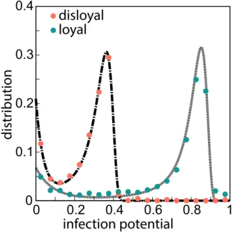
Enfin, pour essayer de mieux comprendre les mécanismes responsables de la perfor-mance de cette méthode, nous avons développé un modèle synthétique de réseau qui garde uniquement les propriétés topologiques de base communes aux deux réseaux réels : hétérogénéité de dégré à tout niveau d’agrégation temporelle, et un niveau de mémoire dans l’évolution, en termes de distribution de loyalty, réglable par un paramètre. Nous avons observé que ces ingrédients sont suffisants pour assurer la précision de nos prévi-sions, et que la mémoire est ce qui règle la puissance prédictive, c’est-à-dire la fraction de nœuds infectés par l’épidémie pour lesquels on a pu produire des prévisions de risque.

infection potential

distr

ibution

disloyal

loyal

Figure R5: potentiel de propagation pour le réseau bovin italien. Les nœuds sont classifiés comme disloyal (✓  0.1, orange) ou loyal (✓ > 0.1, vert). On montre les distributions de la probabilité que un nœud disloyal (loyal), infecté pendant la simulation pour l’année t, soit infecté par la même épidémie pendant l’année t + 1 (potentiel de propagation). On observe que le potentiel de propagation d’un nœud loyal est en moyenne 2.5 plus grand que celui d’un nœud disloyal.

Résumé de la thèse

Conclusions

Dans cette thèse, on a développé de nouvelles méthodes pour estimer et prédire le risque associé à l’émergence d’un nouveau pathogène, à la fois à l’échelle de la popula-tion et à celle de l’hôte, et en utilisant des outils à la fois analytiques et numériques. Nous avons testé ces méthodes dans des milieux différents, tous très pertinents dans le contexte de la santé publique, avec un accent sur les réseaux des mouvements de bovins dans de différents pays européens, pour lesquels nous avons proposé une analyse des caractéristiques topologiques, spatiales et temporelles.

Références

[1] Norman Bailey. The mathematical theory of infectious diseases and its applications. Griffin, London, 1975.

[2] R M Anderson and Robert M May. Infectious Diseases of Humans : Dynamics and Control. Oxford University Press, 1992.

[3] Daryl Daley. Epidemic modelling : an introduction. Cambridge University Press, Cambridge New York, 1999.

[4] Matt J. Keeling and P. Rohani. Modeling Infectious Diseases in Humans and Ani-mals. Princeton University Press, 2007.

[5] Emilia Vynnycky. An introduction to infectious disease modelling. Oxford University Press, Oxford, 2010.

[6] Ciro Cattuto, Wouter den Broeck, Alain Barrat, Vittoria Colizza, Jean-François Pinton, and Alessandro Vespignani. Dynamics of Person-to-Person Interactions from Distributed RFID Sensor Networks. PLoS ONE, 5(7) :e11596, 2010.

[7] Marcel Salathé and James H Jones. Dynamics and Control of Diseases in Networks with Community Structure. PLoS Comput Biol, 6(4) :e1000736, 2010.

[8] Mohammad S Hashemian, Kevin G Stanley, and Nathaniel Osgood. FLUNET : Automated Tracking of Contacts During Flu Season. In WiOpt’10 : Modeling and Optimization in Mobile, Ad Hoc, and Wireless Networks, pages 557–562, Avignon, France, May 2010.

[9] Marcel Salathé, Maria Kazandjieva, Jung Woo Lee, Philip Levis, Marcus W Feld-man, and James H Jones. A high-resolution human contact network for infectious di-sease transmission. Proceedings of the National Academy of Sciences, 107(51) :22020– 22025, 2010.

[10] Lorenzo Isella, Mariateresa Romano, Alain Barrat, Ciro Cattuto, Vittoria Colizza, Wouter Van den Broeck, Francesco Gesualdo, Elisabetta Pandolfi, Lucilla Ravà, Ca-terina Rizzo, and Alberto Eugenio Tozzi. Close Encounters in a Pediatric Ward : Measuring Face-to-Face Proximity and Mixing Patterns with Wearable Sensors. PLOS ONE, 6(2) :e17144, 2011.

[11] Lorenzo Isella, Juliette Stehlé, Alain Barrat, Ciro Cattuto, Jean-François Pinton, and Wouter Van den Broeck. What’s in a crowd ? Analysis of face-to-face behavioral networks. Journal of Theoretical Biology, 271(1) :166–180, 2011.

[12] Juliette Stehlé, Nicolas Voirin, Alain Barrat, Ciro Cattuto, Lorenzo Isella, Jean-François Pinton, Marco Quaggiotto, Wouter Van den Broeck, Corinne Régis, Bruno Lina, and Philippe Vanhems. High-Resolution Measurements of Face-to-Face Contact Patterns in a Primary School. PLOS ONE, 6(8) :e23176, 2011.

[13] Juliette Stehlé, Nicolas Voirin, Alain Barrat, Ciro Cattuto, Vittoria Colizza, Lorenzo Isella, Corinne Regis, Jean-François Pinton, Nagham Khanafer, Wouter Van den Broeck, and Philippe Vanhems. Simulation of an SEIR Infectious Disease Model on the Dynamic Contact Network of Conference Attendees. BMC Medicine, 9(87), July 2011.

[14] Thomas Hornbeck, David Naylor, Alberto M Segre, Geb Thomas, Ted Herman, and Philip M Polgreen. Using Sensor Networks to Study the Effect of Peripatetic Healthcare Workers on the Spread of Hospital-Associated Infections. The Journal of Infectious Diseases, 206(10) :1549–1557, November 2012.

[15] Wouter Van den Broeck, Marco Quaggiotto, Lorenzo Isella, Alain Barrat, and Ciro Cattuto. The making of Sixty-Nine Days Of Close Encounters At The Science Gallery. Leonardo, 45(3) :285, May 2012.

[16] Philippe Vanhems, Alain Barrat, Ciro Cattuto, Jean-François Pinton, Nagham Kha-nafer, Corinne Régis, Byeul-a Kim, Brigitte Comte, and Nicolas Voirin. Estimating Potential Infection Transmission Routes in Hospital Wards Using Wearable Proxi-mity Sensors. PLoS ONE, 8(9) :e73970, 2013.

[17] Julie Fournet and Alain Barrat. Contact Patterns among High School Students. PLoS ONE, 9(9) :e107878, 2014.

[18] Nicolas Voirin, Cécile Payet, Alain Barrat, Ciro Cattuto, Nagham Khanafer, Corinne Régis, Byeul-a Kim, Brigitte Comte, Jean-Sébastien Casalegno, Bruno Lina, and Philippe Vanhems. Combining High-Resolution Contact Data with Virological Data to Investigate Influenza Transmission in a Tertiary Care Hospital. Infection Control & Hospital Epidemiology, 36(03) :254–260, 2015.

[19] Thomas Obadia, Romain Silhol, Lulla Opatowski, Laura Temime, Judith Legrand, Anne C M Thiébaut, Jean-Louis Herrmann, Éric Fleury, Didier Guillemot, and Pierre-Yves Boëlle. Detailed Contact Data and the Dissemination of Staphylococcus aureus in Hospitals. PLoS Comput Biol, 11(3) :e1004170, 2015.

[20] Marta C González, Cesar A Hidalgo, and Albert-László Barabási. Understanding individual human mobility patterns. Nature, 453(7196) :779–782, June 2008. [21] Chaoming Song, Zehui Qu, Nicholas Blumm, and Albert-László Barabási. Limits of

Predictability in Human Mobility. Science, 327(5968) :1018–1021, 2010.

[22] Gautier Krings, Márton Karsai, Sebastian Bernhardsson, Vincent D Blondel, and Jari Saramäki. Effects of time window size and placement on the structure of an aggregated communication network. EPJ Data Science, 1(1) :1–16, 2012.

Résumé de la thèse [23] Mikko Kivelä, Raj Kumar Pan, Kimmo Kaski, János Kertész, Jari Saramäki, and Márton Karsai. Multiscale analysis of spreading in a large communication network. Journal of Statistical Mechanics : Theory and Experiment, 2012(03) :P03005, 2012. [24] Lauri Kovanen, Kimmo Kaski, János Kertész, and Jari Saramäki. Temporal motifs reveal homophily, gender-specific patterns, and group talk in call sequences. Procee-dings of the National Academy of Sciences, 110(45) :18070–18075, 2013.

[25] Zhi-Qiang Jiang, Wen-Jie Xie, Ming-Xia Li, Boris Podobnik, Wei-Xing Zhou, and H Eugene Stanley. Calling patterns in human communication dynamics. Proceedings of the National Academy of Sciences, 110(5) :1600–1605, 2013.

[26] Ming-Xia Li, Vasyl Palchykov, Zhi-Qiang Jiang, Kimmo Kaski, János Kertész, Sal-vatore Miccichè, Michele Tumminello, Wei-Xing Zhou, and Rosario N Mantegna. Statistically validated mobile communication networks : the evolution of motifs in European and Chinese data. New Journal of Physics, 16(8) :83038, 2014.

[27] Michele Tizzoni, Paolo Bajardi, Adeline Decuyper, Guillaume Kon Kam King, Chris-tian M Schneider, Vincent D Blondel, Zbigniew Smoreda, Marta C González, and Vittoria Colizza. On the Use of Human Mobility Proxies for Modeling Epidemics. PLoS Comput Biol, 10(7) :e1003716, 2014.

[28] Pablo Kaluza, Andrea Kölzsch, Michael T Gastner, and Bernd Blasius. The complex network of global cargo ship movements. Journal of The Royal Society Interface, January 2010.

[29] Lijun Sun, Kay W Axhausen, Der-Horng Lee, and Xianfeng Huang. Understanding metropolitan patterns of daily encounters. Proceedings of the National Academy of Sciences, 110(34) :13774–13779, 2013.

[30] Pierre Borgnat, Céline Robardet, Patrice Abry, Patrick Flandrin, Jean-Baptiste Rou-quier, and Nicolas Tremblay. A Dynamical Network View of Lyon’s V\’elo’v Shared Bicycle System. In Animesh Mukherjee, Monojit Choudhury, Fernando Peruani, Niloy Ganguly, and Bivas Mitra, editors, Dynamics On and Of Complex Networks, Volume 2 SE - 13, Modeling and Simulation in Science, Engineering and Technology, pages 267–284. Springer New York, 2013.

[31] Martin Rosvall, Alcides V Esquivel, Andrea Lancichinetti, Jevin D West, and Re-naud Lambiotte. Memory in network flows and its effects on spreading dynamics and community detection. Nat Commun, 5, August 2014.

[32] Ingo Scholtes, Nicolas Wider, René Pfitzner, Antonios Garas, Claudio J Tessone, and Frank Schweitzer. Causality-driven slow-down and speed-up of diffusion in non-Markovian temporal networks. Nat Commun, 5, September 2014.

[33] Ken T D Eames and Matt J. Keeling. Monogamous networks and the spread of sexually transmitted diseases. Mathematical biosciences, 189(2) :115–30, June 2004. [34] Luis E C Rocha, Fredrik Liljeros, and Petter Holme. Information dynamics shape the sexual networks of Internet-mediated prostitution. Proceedings of the National Academy of Sciences of the United States of America, 107(13) :5706–5711, 2010.

[35] R R Kao, Leon Danon, D M Green, and Istvan Z Kiss. Demographic structure and pathogen dynamics on the network of livestock movements in Great Britain. Proceedings of the Royal Society of London B : Biological Sciences, 273(1597) :1999– 2007, August 2006.

[36] Matthew C. Vernon and Matt J. Keeling. Representing the UK’s cattle herd as static and dynamic networks. Proceedings of the Royal Society of London B : Biological Sciences, 276(1656) :469–476, February 2009.

[37] Tom Lindström, Scott A Sisson, Susanna Stenberg Lewerin, and Uno Wennergren. Estimating animal movement contacts between holdings of different production types. Preventive veterinary medicine, 95(1-2) :23–31, June 2010.

[38] Paolo Bajardi, Alain Barrat, Fabrizio Natale, Lara Savini, and Vittoria Colizza. Dynamical Patterns of Cattle Trade Movements. PLoS ONE, 6(5) :e19869, 2011. [39] Mario Konschake, Hartmut H K Lentz, Franz J Conraths, Philipp Hövel, and

Tho-mas Selhorst. On the Robustness of In- and Out-Components in a Temporal Net-work. PLoS ONE, 8(2) :e55223, 2013.

[40] Bhagat Lal Dutta, Pauline Ezanno, and Elisabeta Vergu. Characteristics of the spatio-temporal network of cattle movements in France over a 5-year period. Pre-ventive veterinary medicine, 117(1) :79–94, November 2014.

[41] Alain Barrat, Marc Barthelemy, and Alessandro Vespignani. Dynamical Processes on Complex Networks. Cambridge University Press, 2008.

[42] S N Dorogovtsev, A V Goltsev, and J F F Mendes. Critical phenomena in complex networks. Rev. Mod. Phys., 80(4) :1275–1335, October 2008.

[43] Carter T Butts. Revisiting the Foundations of Network Analysis. Science, 325(5939) :414–416, 2009.

[44] Alessandro Vespignani. Predicting the Behavior of Techno-Social Systems. Science, 325(5939) :425–428, 2009.

[45] M E J Newman. Networks : an introduction. Oxford University Press, Oxford New York, 2010.

[46] Chapter 12 - An Overview of Social Networks and Economic Applications. In Hand-book of Social Economics, volume 1, pages 511–585. 2011.

[47] Alessandro Vespignani. Modelling dynamical processes in complex socio-technical systems. Nat Phys, 8(1) :32–39, January 2012.

[48] Albert-László Barabási. Network science. Cambdridge University Press, Cambridge UK, 2015.

[49] Romualdo Pastor-Satorras and Alessandro Vespignani. Epidemic spreading in scale-free networks. Phys. Rev. Lett., 86(14) :3200–3203, 2001.

[50] M E J Newman. Spread of epidemic disease on networks. Phys. Rev. E, 66(1) :16128, 2002.

Résumé de la thèse [52] Yang Wang, D Chakrabarti, Chenxi Wang, and C Faloutsos. Epidemic spreading in real networks : an eigenvalue viewpoint. In Reliable Distributed Systems, 2003. Proceedings. 22nd International Symposium on, pages 25–34, 2003.

[53] Sergio Gómez, Alexandre Arenas, J Borge-Holthoefer, Sandro Meloni, and Yamir Moreno. Discrete time Markov chain approach to contact-based disease spreading in complex networks. Europhysics Letters, 89(3) :38009, 2010.

[54] Alexei Vazquez, Balázs Rácz, András Lukács, and Albert-László Barabási. Im-pact of Non-Poissonian Activity Patterns on Spreading Processes. Phys. Rev. Lett., 98(15) :158702, April 2007.

[55] José Luis Iribarren and Esteban Moro. Impact of Human Activity Patterns on the Dynamics of Information Diffusion. Phys. Rev. Lett., 103(3) :38702, July 2009. [56] Márton Karsai, Mikko Kivelä, R K Pan, K Kaski, J Kertész, Albert-László Barabási,

and Jari Saramäki. Small but slow world : How network topology and burstiness slow down spreading. Phys. Rev. E, 83(2) :25102, February 2011.

[57] Giovanna Miritello, Esteban Moro, and Rubén Lara. Dynamical strength of social ties in information spreading. Phys. Rev. E, 83(4) :45102, April 2011.

[58] Luis E C Rocha and Vincent D Blondel. Bursts of Vertex Activation and Epidemics in Evolving Networks. PLoS Comput Biol, 9(3) :e1002974, 2013.

[59] Luca Ferreri, Paolo Bajardi, Mario Giacobini, Silvia Perazzo, and Ezio Venturino. Interplay of network dynamics and heterogeneity of ties on spreading dynamics. Phys. Rev. E, 90(1) :12812, July 2014.

[60] Petter Holme and Jari Saramäki. Temporal networks. Physics Reports, 519(3) :97– 125, October 2012.

[61] Petter Holme and Jari Saramäki, editors. Temporal networks. Springer, Berlin New York, 2013.

[62] Petter Holme. Modern temporal network theory : A colloquium. arXiv, 2015. [63] Thilo Gross, Carlos J Dommar D’Lima, and Bernd Blasius. Epidemic Dynamics on

an Adaptive Network. Phys. Rev. Lett., 96(20) :208701, May 2006.

[64] Erik Volz and Lauren Ancel Meyers. Epidemic thresholds in dynamic contact net-works. Journal of The Royal Society Interface, 6(32) :233–241, March 2009.

[65] Michael Taylor, Timothy J Taylor, and Istvan Z Kiss. Epidemic threshold and control in a dynamic network. Phys. Rev. E, 85(1) :16103, January 2012.

[66] Nicola Perra, Bruno Gonçalves, Romualdo Pastor-Satorras, and Alessandro Vespi-gnani. Activity driven modeling of time varying networks. Sci. Rep., 2, June 2012. [67] Suyu Liu, Nicola Perra, Márton Karsai, and Alessandro Vespignani. Controlling Contagion Processes in Activity Driven Networks. Phys. Rev. Lett., 112(11) :118702, March 2014.

[68] Eugenio Valdano, Luca Ferreri, Chiara Poletto, and Vittoria Colizza. Analytical Computation of the Epidemic Threshold on Temporal Networks. Phys. Rev. X, 5(2) :21005, April 2015.

[69] Eugenio Valdano, Chiara Poletto, and Vittoria Colizza. Infection propagator ap-proach to compute epidemic thresholds on temporal networks : impact of immunity and of limited temporal resolution. arXiv, 2015.

[70] Manlio De Domenico, Albert Solé-Ribalta, Emanuele Cozzo, Mikko Kivelä, Yamir Moreno, Mason A Porter, Sergio Gómez, and Alexandre Arenas. Mathematical Formulation of Multilayer Networks. Phys. Rev. X, 3(4) :41022, December 2013. [71] Mikko Kivelä, Alexandre Arenas, Marc Barthelemy, James P Gleeson, Yamir

Mo-reno, and Mason A Porter. Multilayer networks. Journal of Complex Networks, 2(3) :203–271, September 2014.

[72] Eugenio Valdano, Chiara Poletto, Armando Giovannini, Diana Palma, Lara Savini, and Vittoria Colizza. Predicting Epidemic Risk from Past Temporal Contact Data. PLoS Comput Biol, 11(3) :e1004152, 2015.

[73] Piet Van Mieghem. The N-intertwined SIS Epidemic Network Model. Computing, 93(2-4) :147–169, 2011.

[74] Iain Anderson. Foot and Mouth Disease 2001 : Lessons to be Learned Inquiry Report. The Stationery Office, (July), 2002.

[75] T. E. Carpenter, J. M. O’Brien, A. D. Hagerman, and B. A. McCarl. Epidemic and Economic Impacts of Delayed Detection of Foot-And-Mouth Disease : A Case Study of a Simulated Outbreak in California. Journal of Veterinary Diagnostic Investigation, 23(1) :26–33, January 2011.

[76] L H Taylor, S M Latham, and Mark E J Woolhouse. Risk factors for human disease emergence. Philosophical Transactions of the Royal Society B : Biological Sciences, 356(1411) :983–989, July 2001.

[77] Matt J. Keeling, Mark E J Woolhouse, Darren J Shaw, Louise Matthews, Margo Chase-Topping, Dan T Haydon, Stephen J Cornell, Jens Kappey, John Wilesmith, and Bryan T Grenfell. Dynamics of the 2001 UK Foot and Mouth Epidemic : Stochastic Dispersal in a Heterogeneous Landscape. Science, 294(5543) :813–817, 2001.

[78] Matt J. Keeling. Models of foot-and-mouth disease. Proceedings of the Royal Society of London B : Biological Sciences, 272(1569) :1195–1202, June 2005.

[79] A-F Viet, C Fourichon, and H Seegers. Review and critical discussion of assump-tions and modelling opassump-tions to study the spread of the bovine viral diarrhoea virus (BVDV) within a cattle herd. Epidemiology and infection, 135(5) :706–721, 2007. [80] Aurélie Courcoul and Pauline Ezanno. Modelling the spread of Bovine Viral

Diar-rhoea Virus (BVDV) in a managed metapopulation of cattle herds. Veterinary Microbiology, 142(1-2) :119–128, 2010.

[81] Mark Tinsley, Fraser I Lewis, and Franz Brülisauer. Network modeling of BVD transmission. Veterinary research, 43(1) :11, January 2012.

[82] L.M. O’Reilly and C.J. Daborn. The epidemiology of Mycobacterium bovis infections in animals and man : A review. Tubercle and Lung Disease, 76 :1–46, August 1995.

Résumé de la thèse [83] Robin A. Skuce, Adrian R. Allen, and Stanley W. J. McDowell. Herd-level risk fac-tors for bovine tuberculosis : A literature review. Veterinary Medicine International, 2012 :621210, 2012.

[84] Ellen Brooks-Pollock, Gareth O. Roberts, and Matt J. Keeling. A dynamic model of bovine tuberculosis spread and control in Great Britain. Nature, 511(7508) :228–231, July 2014.

[85] V Taleski, L Zerva, T Kantardjiev, Z Cvetnic, M Erski-Biljic, B Nikolovski, J Bosn-jakovski, V Katalinic-Jankovic, A Panteliadou, S Stojkoski, and T Kirandziski. An overview of the epidemiology and epizootology of brucellosis in selected countries of Central and Southeast Europe. Veterinary Microbiology, 90(1-4) :147–155, Decem-ber 2002.

[86] T England, L Kelly, R D Jones, A MacMillan, and M Wooldridge. A simulation model of brucellosis spread in British cattle under several testing regimes. Preventive veterinary medicine, 63(1-2) :63–73, April 2004.

[87] E Díaz Aparicio. Epidemiology of brucellosis in domestic animals caused by Bru-cella melitensis, BruBru-cella suis and BruBru-cella abortus. Revue scientifique et technique (International Office of Epizootics), 32(1) :43–51, 53–60, 2013.

[88] V Moennig, G Floegel-Niesmann, and I Greiser-Wilke. Clinical Signs and Epide-miology of Classical Swine Fever : A Review of New Knowledge. The Veterinary Journal, 165(1) :11–20, January 2003.

[89] S Costard, L Mur, J Lubroth, J M Sanchez-Vizcaino, and D U Pfeiffer. Epidemiology of African swine fever virus. Virus research, 173(1) :191–7, April 2013.

PHD THESIS

Computing the vulnerability of

time-evolving networks to infections

Eugenio Valdano

Sorbonne Universit´es, UPMC Univ Paris 06, INSERM, Institut Pierre Louis d’´Epid´emiologie et de Sant´e Publique (IPLESP UMRS 1136), F75012, Paris, France.

Computing the vulnerability of time-evolving networks to infections

Research articles published as first author contained in this thesis

• Eugenio Valdano, Luca Ferreri, Chiara Poletto, and Vittoria Colizza. Analytical Computation of the Epidemic Threshold on Temporal Networks. Physical Review X, 5(2):21005, 2015.

Cited in this thesis as [1].

• Eugenio Valdano, Chiara Poletto, Armando Giovannini, Diana Palma, Lara Savini, and Vittoria Colizza.

Predicting Epidemic Risk from Past Temporal Contact Data. PLoS Computational Biology, 11(3):e1004152, 2015.

Cited in this thesis as [2].

Research articles submitted as first author contained in this thesis

• Eugenio Valdano, Chiara Poletto, and Vittoria Colizza.

Infection propagator approach to compute epidemic thresholds on temporal net-works: impact of immunity and of limited temporal resolution.

2015. - under review. Cited in this thesis as [3].

Quare habe tibi quicquid hoc libelli qualecumque; quod, patrona virgo, plus uno maneat perenne saeclo.

Abstract

Infectious disease modeling represents a powerful tool for assessing the vulnerability of a population to the introduction of a new infectious pathogen. The increased availability of highly resolved data tracking host interactions is making epidemic models potentially increasingly accurate. Integrating into them all the features emerging from these data, however, still represents a challenge. In particular, the interaction between disease dy-namics and the time evolution of contact structures has been shown to impact the way pathogens spread. Specifically, it changes the conditions that lead to the wide-spreading regime, as encoded in epidemic threshold, which is the critical transmissibility value above which the epidemic breaks out. Up to now, through the formalism of tempo-ral networks, researchers have characterized the epidemic threshold on time evolving contact structures only through numerical approaches or in specific settings. Using a multilayer formalism, we analytically compute the epidemic threshold on a generic tem-poral network, accounting for several di↵erent disease features. We use this methodology to assess the impact of time resolution and network duration on the estimation of the threshold, given the importance that these features have in setting up an optimal data collection strategy. We introduce several epidemiologically relevant datasets, and in par-ticular we analyze the networks of cattle trade movements, highlighting the features that can influence disease spreading. Then we use the analytical tools we have developed to assess the global vulnerability of di↵erent systems to pathogen introduction, focusing on Italian cattle trade movements, and on a network of human sexual contacts. Data collection strategies often inform us only about past network configurations, and that limits our prediction capabilities. We face this by developing a data-driven methodology for predicting targeted epidemic that relies only past contact data, and apply to real and synthetic networks. Our work provides new methodologies for assessing and predicting the risk associated to an emerging pathogen, both at the population scale and targeting specific hosts. We develop and test them in a wide variety of contexts, making our results widely applicable.

Contents

. Introduction 13

1. Epidemics on static networks 17

1.1. Compartmental models . . . 17 1.2. Homogeneous mixing . . . 20 1.3. Networks . . . 21 1.4. Epidemics on networks . . . 22 1.5. The epidemic threshold . . . 23 1.5.1. Homogeneous mixing: R0 . . . 26

1.5.2. Static and annealed networks . . . 29

2. Temporal networks 33

2.1. Definition and basic properties . . . 34 2.2. Representations . . . 35 2.3. Statistical properties . . . 40 2.4. Datasets . . . 41 2.5. Synthetic models of temporal networks . . . 43 2.6. Null models for temporal networks . . . 47 2.7. Epidemics on temporal networks . . . 48

3. The epidemic threshold on temporal networks 51

3.1. A novel multilayer mapping of network evolution and disease dynamics . . 52 3.2. Article: Analytical computation of the epidemic threshold on temporal

networks . . . 55 3.3. Article: Infection propagator approach to compute epidemic thresholds on

temporal networks: impact of immunity and of limited temporal resolution 56 3.4. Continuous time . . . 57

3.5. Latency . . . 61 3.6. Conclusion . . . 66

4. Cattle trade movements 69

4.1. Defining the network . . . 70 4.2. Static topologic properties . . . 72 4.3. Temporal patterns . . . 74 4.4. Geographic patterns . . . 84 4.5. Conclusion . . . 87

5. Targeted risk prediction 89

5.1. Vulnerability of Italian cattle trade network . . . 90 5.2. Sexual contact network: how latency influences vulnerability . . . 95 5.3. Article: Predicting epidemic risk from past temporal contact data . . . . 96

. Conclusions and perspectives 97

A. Appendix 99

A.1. Networks - essential glossary . . . 99 A.2. Tensor representation of temporal networks . . . 100 A.3. Discrete Fourier Transform . . . 101 A.4. R0 from di↵erential equations . . . 102

Introduction

Infectious diseases represent a major burden on welfare and society. They directly threaten human health, and impact economy and development. In developing coun-tries, they represent the top cause of death [4], and pose a particularly heavy burden on child health, with pneumonia, diarrhea and malaria together accounting for more than 60% percent of child deaths [5]. Even in the developed World, where most deaths are due to non-infectious diseases, the situation may worsen in the near future. Bacteria strains are developing antibiotic resistance at a quicker pace than we can come up with new drugs [6], and vector-borne diseases (for instance, Dengue Fever [7]) are now reaching areas in which they were previously absent, as climate change impacts vector ecology. Finally, the ever more globalized World we live in is prone to breakouts of pathogens with pandemic potential, like SARS (2003) [8–10], H1N1 flu (2009) [11–15], or, more recently MERS CoV [16–19] and Ebola [20–23]. In the fight against infectious diseases, mathematical models have become an important tool, as they provide tools to reduce the number of infections, optimally allocate limited resources, react promptly to emer-gencies, and implement targeted containment strategies. Ever since their introduction in 1927 by Kermack & McHendrick [24–26], these models are based on the assumption that disease transmission and progression can be translated into a relative simple set of mechanistic rules that can be adapted to pathogens with very diverse pathophysiology, clinical symptoms, and causative agents (bacteria, viruses, etc.). The epidemic is then an emerging collective behavior of the “microscopic” interactions among hosts [27–31]. This framework has allowed researchers to apply and develop several tools and tech-niques borrowed from mathematics and statistical physics. Up until two decades ago, however, the use of mathematical models in public health was limited by the lack of data concerning human interactions. Simplified and coarse-grained assumptions limited model applicability to real scenarios. The picture has dramatically changed in the last years, with the outbreak of data science. The development of both new hardware and software technologies has made it possible to track contacts and transports relevant for

the spread of diseases in an extremely accurate and almost unsupervised way. We now have detailed records of how people interact in di↵erent settings, and at di↵erent scales, from face-to-face proximity encounters [32–45], to mobility patterns [46–58], to sexual contacts [59, 60]. Detailed data do not concern only human activities: we can now keep track of livestock displacements between farms, which are spreading routes for many diseases threatening animal health, economy, and ultimately human health [61–66].

This “data deluge”1 _{has radically transformed infectious disease modeling, proving}

to be both a huge resource and a great challenge. High resolution data have made it possible to model entire populations down to single individuals [67–73], providing tailored real-time predictions of epidemic outbreaks [15, 74, 75]. These simulations schemes are e↵ective and perform well in specific settings, but cannot provide a general understanding of the unfolding of epidemic processes. New theoretical tools have been developed in order to deal with the complexity of interaction structures, treating diseases as dynamic processes on networks [76–83]. Networks have indeed become a common and successful tool to model populations in terms of nodes (hosts) and links (interactions among hosts) of a graph [84–86]. This has made it possible to use all the tools already developed in statistical physics, graph theory, and dynamical systems, to the context of infectious diseases.

An important feature emerging from this huge amount of data is that contacts are not fixed in time during the spread of the disease, but evolve in time. The complex interplay between network evolution and disease di↵usion has been proven to impact the outcome of the epidemic process, in several di↵erent contexts [39, 87–92]. This is due to time correlations between contacts, that determine the shape and amount of routes along which the disease can spread, and make traditional risk proxies, developed for static contact patterns, insufficient to characterize this new phenomenology [64, 93].

As a result, a methodology that aims at assessing the threat a specific pathogen poses to a population must account for the temporal evolution of contacts within that popula-tion. This calls for new theoretical tools to handle the interaction between the dynamics of network evolution, and the spread of the pathogen. Temporal networks represent an e↵ective framework to model time-evolving contact patterns [94–96], but their interplay with spreading dynamics has so far been investigated only though numerical approaches, or in controlled settings [92, 97–101]. In the first part of our work we focus on assessing

Computing the vulnerability of time-evolving networks to infections

the vulnerability of a system to a disease, in term of its epidemic threshold, i.e., the critical value of disease transmissibility above which the epidemic breaks out. We in-troduce a new way of representing the unfolding of a disease on a time-evolving contact structure in terms of a multilayer network [102, 103], and use it to analytically compute the epidemic threshold on a generic temporal network. Our computation can account for various disease features, like immunity, waning of immunity and latency period. We then focus on particular datasets that carry a notable epidemiological relevance. Specifically, we provide a comparative analysis of the network of cattle trade movements in three European countries, highlighting the structural features that can impact the spread of an epidemic. In the last part of the thesis we develop a risk assessment analysis on these specific datasets, focusing on particular classes of diseases. Thanks to our theoretical findings, we can use the threshold as a measure of global network risk. Then, we focus on a more targeted, host-centered, risk analysis. Given that, for many systems, contacts are not reported in real time, the datasets that are commonly available inform us on the structure of contacts in the past, and that limits our prediction capabilities. We thus develop a data-driven methodology that, in case of a future epidemic outbreak of a certain pathogen, is able to provide the risk a particular host will be hit, by relying only to past contact data. We apply this methodology to di↵erent real scenarios, and develop a generative network model to test which structural features of contacts determine the performance of our prediction.

The goal of this thesis is thus to present new tools to assess and predict the risk asso-ciated to the introduction of a pathogen onto a population, accounting for the dynamic evolution of the pattern of contacts among hosts. We do that through new analytical tools that are able to handle the interplay between network and disease dynamics, and through data-driven analyses and models. The variety of datasets and disease models we consider, albeit being a simplification of the actual progression of real pathogen, makes our findings applicable to various contexts and scenarios.

In Chapter 1 we introduce the basics of epidemic modeling and networks. We also define the epidemic threshold, and show how to compute it in di↵erent settings. In Chapter 2 we define temporal networks, their epidemiological relevance, and their repre-sentations. We also introduce some datasets that will be used in the following chapters. We then describe some generative models and reference models for temporal networks. In Chapter 3 we develop our methodology for computing the epidemic threshold on temporal networks. We extend it to generic networks, and di↵erent disease models.

We also assess the impact of temporal aggregation of contact data, and the length of the period of data collection in empirical settings. This chapter includes two research articles: Analytical computation of the epidemic threshold on temporal networks, pub-lished on Physical Review X [1], and Infection propagator approach to compute epidemic thresholds on temporal networks: impact of immunity and of limited temporal resolution, currently under review [3]. In Chapter 4 we provide a comparative analysis of cattle dis-placement networks in three European countries. In Chapter 5 we compute epidemic risk in real settings, cattle trade movements (Chapter 4) and sexual contact network (Chap-ter 2 and [60]). In this chap(Chap-ter we develop and apply our framework for computing node epidemic risk from past contact data, contained in our article Predicting Epidemic Risk from Past Temporal Contact Data, published in PLoS Computational Biology [2].

1. Epidemics on static networks

Infectious diseases vary widely in their pathophysiology, clinical symptoms and etiology, resulting in diverse progression and transmission patterns. Viral diseases, like influenza, measles, chicken pox, usually confer permanent immunity after recovery, while bacterial diseases (tuberculosis, syphilis) allow multiple re-infections of the same host. Many diseases are transmitted by direct contact between hosts, while others require vectors, such as malaria or bluetongue. Some, like cholera, require the ingestion of contaminated water and food. Such diversity calls for modeling approaches that are general and versatile enough to be adapted to each specific ailment, and still be a realistic description of its epidemiological features [104]. This is commonly achieved through compartmental models, which will be the first argument of this chapter. We will then explain how to account for the contact structure of the host population, and how compartmental models are adapted to complex population structures. Finally, we will investigate what are the conditions that, following a pathogen introduction in a susceptible population, lead to an epidemic outbreak. We will formalize this concept in terms of epidemic threshold, and show how to compute it for several contact structures.

1.1. Compartmental models

In principle, the mathematical description of an infectious disease can explore di↵erent scales, from describing pathogen population dynamics within a host, to ecological mod-els that predict incidence in a population. We are interested in modeling the spread of a disease on a host population, so we consider the health status of a host as the elementary building block of our modeling approach. In particular, we assume that the health status can be described as a discrete set of states (compartments). The two compartments that characterize every epidemic model are susceptible (S) to being infected, and infectious (I), i.e., infected and contagious. Another compartment commonly used is recovered (R), i.e., immune to the disease. Hosts in the population are divided into compartments,

ac-cording to their health status [28, 105], and disease progression is modeled in terms of a set of interaction and transition rules among compartments. The simplest conceivable model is the susceptible-infected (SI). In the SI model, infectious hosts infect their sus-ceptible neighbors with probability , and no recovery is possible. Despite its extreme simplicity, the SI model can be used, for instance, to approximate the initial stage of an outbreak (Section 5.3 and [2]). Other widely used models are the susceptible-infectious-susceptible (SIS) and susceptible-infectious-susceptible-infectious-recovered (SIR) models. In both models, infectious hosts infect their susceptible neighbors with probability . In addition, they recover with probability µ, going either back to the susceptible state (SIS), or to the recovered state (SIR). In the SIR model recovered hosts are immune to re-infection. Probabilities are usually defined in discrete time; when time is continuous we have rates instead of probabilities, i.e., probabilities per infinitesimal time interval (see also Sec-tion 3.3 and [3]). The success of these two models is due to two aspects. Firstly their simplicity and their small number of free parameters make them analytically treatable, and their results provide a general understanding of infection dynamics. Secondly, they have proven adequate to model a wide range of diseases under simplifying assumptions. SIS model applies quite well to bacterial infections (see, for instance, hospital acquired MRSA [45], or STD’s [91]), while SIR model works well with viral diseases, like flu, chicken pox [28], cattle Foot-and-Mouth [106]. More elaborate compartmental models account of more complex infection dynamics. Among them, we describe two that we will use in this thesis. The first is the SIRS model. Its progression is analogous to SIR model, but recovered individuals lose their immunity with probability !, going back to susceptible state. SIR model can indeed be seen as a particular case of SIRS, when ! = 0. The last model we use is the SEIS model. Many ailments are characterized by a latency period, which is a time lag between being infected, and becoming infectious. We can take this feature into account by adding a new compartment to the model, E (Exposed). A susceptible agent is infected by an infectious neighbor, and becomes ex-posed. It then turns infectious with a probability ✏. From then, the progression is the same as the SIS model. Figure 1.1 schematically summarizes all the models we use in this thesis. For a detailed description of compartmental models we refer to traditional textbooks [27–31].

Computing the vulnerability of time-evolving networks to infections

SIS

SIR

SIRS

SEIS

λ

λ

λ

μ

μ

μ

ε

λ

μ

ω

SIS

S E

I R

SIR

SIRS

SEIS

λ

λ

λ

μ

SI

_λ

μ

μ

ε

λ

μ

ω

Figure 1.1.: Compartmental models. The first row describes the four compartments used. Susceptible is in blue, infectious in red, recovered in gray, and exposed in yellow. Dynamics of SI, SIS, SIR, SIRS and SEIS is then described. Arrows showing transitions from one compartment to the other are pictured with the respective probability. The red (infectious) smaller point close to indicates that infection requires interaction with an infectious agent. All other processes are spontaneous one-body transitions.

1.2. Homogeneous mixing

In general, the choice of compartmental model, and the values of the parameters, are informed by the epidemiology of the specific disease under study. The goal of infectious disease modeling is to uncover and characterize the macroscopic behavior emerging from applying such model to a population interacting in a certain way. In order to do that, it is necessary to have information about the structure of contacts along which the disease spreads.

The simplest framework is homogeneous mixing, which assumes no specific contact structure. Every host in the population has the same probability of being in contact with any other host. Despite its simplicity, homogeneous mixing still represents a suc-cessful approximation in many contexts, especially within patches of meta-population models [15, 107–111].

The traditional way to couple compartmental models to homogeneous mixing is repre-sented by deterministic di↵erential equations, interpreting pathogen spread as a reaction process. These equations compute the number of hosts in a compartment as a function of time. Let S(t), I(t), R(t) be the number of susceptible (infectious, recovered) individ-uals at time t. We call N the population size, and k the number of contacts every host establishes. The equations of the SIS model are

8 < : ˙ S = _NkSI + µI; ˙ I = _NkSI µI. (1.1)

For the SIR model are instead 8 > > > < > > > : ˙ S = _NkSI; ˙ I = _NkSI µI; ˙ R = µI. (1.2)

Last line in both Equation 1.1 and Equation 1.2 is redundant if we assume a fixed population ( ˙N _{⌘ 0).}

Deterministic di↵erential equations, however, have two important limitations. They treat the number of infected agents as a continuous variable, and they do not account for stochastic e↵ects. In other words, they do not consider hosts as individual entities, which have a certain probability of transmitting to a contact, or change infection status. As a result, di↵erential equations produce accurate predictions only in large populations (in

Computing the vulnerability of time-evolving networks to infections

the limit N _{! 1). Real populations, however, often cannot be treated as infinite, and} stochastic e↵ects kick in. They not only quantitatively change the predictions, but have conceptual implications in defining what we mean by the persistence of an epidemic. One way to account for stochastic e↵ects in the framework of homogeneous mixing is through branching processes [112–114]. In a SIS branching process, any infectious host in a given generation produces a random number of infectious hosts, sampled from a given distribution, which make up the next generation. In practice we seed a certain number of infectious hosts (first generation), they then will produce a certain number of infectious (second generation), and so on.

1.3. Networks

Epidemiologists have been reconstructing who had been in contact with whom during a particular time frame through surveys and questionnaires, asking, for instance, to list list all people you had met that particular day. This strategy has been used for di↵erent types of contacts, like face-to-face proximity [115–120], sexual encounters [121], and needle share among injection drug users [122–124]. These data allowed researchers to uncover features of human interactions, which prompted the need of going beyond the homogeneous mixing assumption. Researchers found out that these these complex contact structures could be represented as networks [76, 80, 82, 83, 125, 126].

A network is a representation of an interacting population, in terms of a mathematical entity, the graph [84–86, 127, 128]. A graph is composed of a set of nodes (vertices), and links (edges) that connect pairs of nodes. In our context, nodes represent the hosts of our population, and links represent the interactions relevant to the spread of the disease. The first elementary concept that arises is the one of neighbor and neighborhood. Two nodes are neighbors if there is a link among them, and the neighborhood of a node is the set of its neighbor nodes. Networks can be undirected, when links represent mutual interactions, or directed, like in the case of transport networks. In other words, in directed networks the proposition “i is contact with j” does not imply “j is contact with i”. Furthermore, links can be binary relationships, or weighted by an intensity factor, modulating force-of-infection (weighted networks [128]). One of the advantages of the network approach is that a graph has a natural algebraic representation in terms of adjacency matrix [129, 130]. Given a network with N nodes labeled as i, j = 1_{· · · N, its} adjacency matrix A has entry Aij = 1 if i is connected to j, and zero otherwise. If the

network is undirected, then A is symmetric (A = A†); if the network is weighted, Aij can

assume values other than 0, 1, encoding link weights. One of the most important graph-theoretical measures is degree of a node [80], i.e., the number of connections this node establishes with other nodes. For directed networks, we discriminate between incoming and outgoing degree, and for weighted networks we also introduce strength of a node, i.e. the sum of the weights of its links. Networks are often characterized in terms of their degree distribution, i.e., the statistical distribution of node degrees. When nodes establish links randomly, the resulting degree distribution is Poisson-like, with small dispersion around a mean value [80, 128]. On the other hand, networks with deeply non random connection patterns exhibit heterogeneous degree distributions, with large, sometimes diverging, variance. The most popular heterogeneous distribution in this context is the power-law P (k)_{⇠ k} [131,132], as many real networks are found to have degree distribution closely related to it. We summarize essential definitions of network theory in Appendix A.1. For a detailed introduction to networks, we refer to the books by Newman [80] and Barab´asi [83].

1.4. Epidemics on networks

In order to model the spread of a disease on a network, we choose the appropriate compartmental model. Then we infect a limited set of nodes (epidemic seeds). Assuming discrete time, at each time step all infectious nodes infect their neighbors with probability equal to disease transmissibility (see Figure 1.1). At the same time, in each node the disease progresses as required by the chosen model. For instance, in the case of SIR model, at each time step every infectious node recovers with probability µ.

Many features of real interaction networks have proven to dramatically impact the way diseases spread. The simplest, yet extremely crucial, among these features is the presence of hubs (large degree nodes). Heterogeneous degree distributions generally make the network more vulnerable to disease invasion and persistence, with respect to homogeneous mixing [76,133–136]. As soon as the pathogen is able to infect the hubs, it gets access to a large part of the network, making its containment more difficult. Hubs also make the network more vulnerable to disease invasion (see [133] and Section 1.5.2), and more difficult to immunize. Strategies based on homogeneous mixing predicate that as soon as you immunize a critical fraction of the population, e.g. through vaccina-tion, the disease is no longer able to turn epidemic. This phenomenon is called herd