Cognitive Optical Network Architecture in Dynamic
Environments
by
Xijia Zheng
E.E., Massachusetts Institute of Technology (2017)
S.M., Massachusetts Institute of Technology (2015)
B.Eng., The University of Hong Kong (2014)
Submitted to the Department of Electrical Engineering and Computer
Science
in partial fulfillment of the requirements for the degree of
Doctor of Philosophy in Computer Science and Engineering
at the
MASSACHUSETTS INSTITUTE OF TECHNOLOGY
May 2020
c
○ Massachusetts Institute of Technology 2020. All rights reserved.
Author . . . .
Department of Electrical Engineering and Computer Science
May 15, 2020
Certified by . . . .
Vincent W. S. Chan
Joan and Irwin Jacobs Professor of Electrical Engineering and
Computer Science
Thesis Supervisor
Accepted by . . . .
Leslie A. Kolodziejski
Professor of Electrical Engineering and Computer Science
Chair, Department Committee on Graduate Students
Cognitive Optical Network Architecture in Dynamic
Environments
by
Xijia Zheng
Submitted to the Department of Electrical Engineering and Computer Science on May 15, 2020, in partial fulfillment of the
requirements for the degree of
Doctor of Philosophy in Computer Science and Engineering
Abstract
Emerging network traffic requires a more agile network management and control system to deal with the dynamic network environments than today’s networks use. The bursty and large data transactions introduced by new technological applications can cause both high costs and extreme congestion in networks. The prohibitive cost of massive over-provisioning will manifest as huge congestions during peak demand periods. The network management and control system must be able to sense the traffic changes and reconfigure in a timely manner (in tens of milliseconds instead of minutes or hours) to use network resources efficiently. We propose the use of cognitive techniques for fast and adaptive network management and control of future optical networks. The goal of this work is to provide timely network reconfigurations in response to dynamic traffic environments and prevent congestion from building up.
We make a simplified model of the expected traffic arrival rate changes as a multi-state Markov process based on the characteristics of the dynamic, bursty, and high granularity traffic. The traffic is categorized into different network traffic environ-ments by the length of the network coherence time, which is the time that the traffic is unvarying. The tunneled network architecture is adopted due to its supremacy in reducing the control complexity when the traffic volume is at least one wavelength.
In the long coherence time regime where traffic changes very slowly, the traffic detection performances of two Bayesian estimators and a stopping-trial (sequential) estimator are examined, based on the transient behaviors of networks. The stopping-trial estimator has the fastest response time to the changes of traffic arrival statis-tics. We propose a wavelength reconfiguration algorithm with continuous assessment where the system reconfigures whenever it deems necessary. The reconfiguration can involve addition or subtraction of multiple wavelengths. Using the fastest detection and reconfiguration algorithm can reduce queueing delays during traffic surges with-out over-provisioning and thus can reduce network capital expenditure and prevent wasting resources on erroneous decisions when surges occur.
For traffic with moderate coherence time (where traffic changes at a moderate rate) and the short coherence time (where traffic changes quickly), the
stopping-trial estimator still responds to the traffic changes with a short detection time. As long as the inter-arrival times of traffic transactions are independent, the algorithm is still optimum. The algorithm provides no prejudice on the exact network traffic distribution, avoiding having to sense and estimate detailed arrival traffic statistics.
To deal with fast-changing traffic, we model the transient convergent behaviors of network traffic drift as a result of traffic transition rate changes and validate the feasibility and utility of the traffic prediction. In a simple example when the net-work traffic rate changes monotonically in a linear model, the sequential maximum likelihood estimator will capture the traffic trend with a small number of arrivals. The traffic trend prediction can help to provide fast reconfiguration, which is very important for maintaining quality of service during large traffic shifts.
We further investigate the design of an efficient rerouting algorithm to maintain users’ quality of service when the incremental traffic cannot be accommodated on the primary path. The algorithm includes the fast reconfiguration of wavelengths in the existing lit and spatially routed fibers, and the setting up and lighting of new fibers. Rerouting is necessary to maintain users’ quality of service when the queueing delay on the primary path (determined by shortest path routing) exceeds the requirement. Our algorithm triggers reconfiguration when a queueing delay threshold is crossed on the primary path. The triggering by a threshold on the queueing delay is used due to its simplicity, and it is directly measurable by the exact traffic transaction sizes and the queue size, which reflect both the current network traffic environment and the network configurations. A dynamic rerouting algorithm implemented with a shortest-path algorithm is proposed to find the secondary shortest-paths for rerouting. We make the conjecture that it is desirable that the alternate paths for rerouting have small numbers of hops and are disjoint with other busy paths when the hops on the path are independent. In addition, the conjecture suggests that a good candidate network topology should have high edge-connectivity. Wavelength reservation for rerouted traffic does not maximize wavelength utilization. We make the conjecture that traffic with different sizes should be broken up into multi-classes with dedicated partitioned resources and the queueing delay should be normalized by the transmission time for rerouting triggering to realize better network utilization.
Thesis Supervisor: Vincent W. S. Chan
Title: Joan and Irwin Jacobs Professor of Electrical Engineering and Computer Sci-ence
Acknowledgments
First and foremost, I would like to express my deepest gratitude to my research advisor, Professor Vincent W. S. Chan, for his knowledge, expertise, support, and patience. His emphasis on practical design, creative thinking and precise communi-cation continues to be a great inspiration to me. Moreover, his dedicommuni-cation and advice have been invaluable and will continue to support me in life.
I would also like to thank Dr. Richard Barry and Professor Vivienne Sze for carving out time to join my thesis committee. I am deeply grateful to them for providing invaluable feedback for my research and assisting in polishing this work.
I would like to thank my fellow group mates: Lei Zhang, Henna Huang, Matthew Carey, Manishika Agaskar, Shane Fink, Arman Rezaee, John Metzger, Antonia Feffer, Esther Jang, Andrew Song, and Junior Weerachai Neeranartvong. All of them have made my time in the group enjoyable and wonderful.
I would like to thank my friends both near and far. I am so grateful for their friendship and encouragement.
Last but not the least, I would like to thank my parents for their unconditional love, guidance, and unwavering support. This thesis is dedicated to them.
Contents
1 Introduction 19
1.1 Increasing Traffic . . . 19
1.2 Cognitive Optical Networking . . . 22
1.3 Design Goals . . . 26
1.4 Cognitive Optical Network Design Submodules . . . 28
1.5 Thesis Scope and Organization . . . 29
2 Dynamic Traffic Environment, Tunneled Architecture, and Recon-figurations 33 2.1 Dynamic Traffic Model . . . 33
2.1.1 All-to-all Stochastic Traffic . . . 34
2.1.2 Multi-state Markov Arrival Rate . . . 35
2.1.3 Network Coherence Time . . . 38
2.2 Tunneled Architecture . . . 39
2.3 Traffic Load . . . 40
2.4 Reconfigurations . . . 41
3 Long Coherence Time Traffic Environment 45 3.1 Two Bayesian Estimators . . . 46
3.1.1 Fixed-Time Estimator ^𝜆𝑇(𝑡) . . . 48
3.1.2 Fixed-Count Estimator ^𝜆𝑁(𝑡) . . . 51
3.1.3 Comparison of the Two Bayesian Estimators . . . 54
3.3 Network Transient Behaviors . . . 64
3.3.1 Sampled-Time Markov Chain Approximation . . . 66
3.3.2 𝑀/𝑀/1/𝑋 Queue Transient Behavior Approximation . . . 68
3.3.3 Transient Behavior of the Queue . . . 69
3.3.4 Detection Time 𝜏1 . . . 75
3.3.5 Peak Queueing Delay Γ𝑝𝑒𝑎𝑘 . . . 79
3.3.6 Queue settling time 𝜏2 . . . 82
3.4 Cost-Driven Network Reconfiguration Scheme . . . 84
3.4.1 Network Operating Cost Model . . . 85
3.4.2 Multiple Wavelengths Addition and Subtraction . . . 87
3.5 Chapter 3 Summary . . . 90
4 Moderate Coherence Time Traffic Environment 93 4.1 Validation of Stopping-Trial Estimator . . . 94
4.1.1 Uncertain Start Counting Point . . . 95
4.1.2 Detection Performance in Different Environments . . . 97
4.2 Detection Performance in Moderate Network Coherence Time Envi-ronment . . . 99
4.3 Reconfiguration in Moderate Coherence Time Traffic Environment . . 103
4.4 Chapter 4 Summary . . . 103
5 Short Coherence Time Traffic Environment 105 5.1 Fast Detection in Short Network Coherence Time Environment . . . . 106
5.2 Network Drifting Time . . . 108
5.3 Prediction of the Network Traffic Drifting Trend . . . 114
5.4 Summary of Chapter 5 . . . 118
6 Rerouting 121 6.1 Rerouted Traffic and Shortest-Path Rerouting . . . 122
6.2 Blocking of Secondary Paths for Rerouting . . . 124
6.2.2 Topology Recommendation for Efficient Rerouting . . . 128
6.3 Wavelength Reservation for Rerouted Traffic . . . 131
6.4 Delay Threshold to Reroute . . . 134
6.4.1 Triggering Algorithm with the Delay Threshold . . . 135
6.4.2 Performance for Node Pair with Single Wavelength . . . 137
6.4.3 Performance for Node Pair with Multiple Wavelengths . . . . 140
6.5 Summary of Chapter 6 . . . 143
List of Figures
1-1 Cognitive all-optical network concept with optical gateways between hierarchical subnet, peering gateway control points and cognitive en-gine sensing and interacting with multiple layers for network control. Reproduced from [7, 9]. . . 24 1-2 An agile control plane architecture of cognitive network management
and control system. Reproduced from [8, 10]. . . 25 2-1 All-to-all dynamic traffic. . . 35 2-2 Multi-state embedded Markov chain transition of the traffic arrival rate
𝜆(𝑡). . . 37 2-3 An example of an all-to-all tunneled network connection between node
pairs in the form of wavelengths. (a) All-to-all tunneled network topol-ogy; (b) Reconfigurable wavelength assignment. . . 40 2-4 The traffic transmission of three network reconfiguration options. (a)
The dynamic wavelength addition or subtraction on the primary path. Traffic will be transmitted on the primary path. (b) The rerouting of the incremental traffic. Part of the traffic will be transmitted on paths other than the primary path. (c) The new fiber setup on the primary path. Traffic will be transmitted on the primary path. . . 42 3-1 Two-state embedded Markov chain transition of the traffic arrival rate
𝜆(𝑡). . . 47 3-2 The comparison of detection shapes of ^𝜆𝑇(𝑡) and ^𝜆𝑁(𝑡) in a single run.
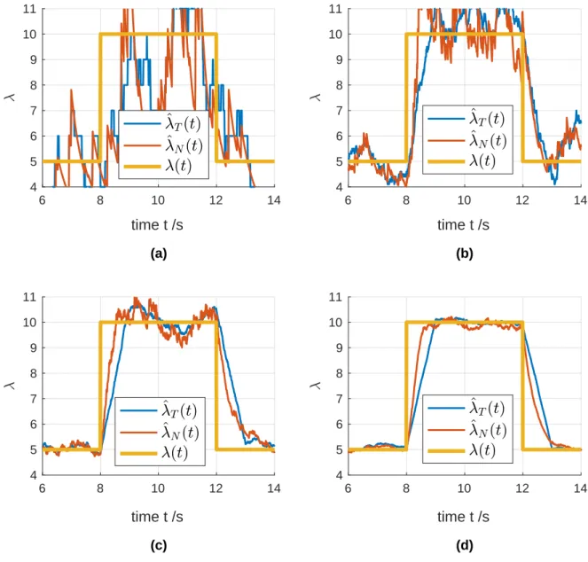
3-3 The comparison of the average detection results over different numbers of runs of ^𝜆𝑇(𝑡) and ^𝜆𝑁(𝑡): (a) a single run; (b) 10 runs; (c) 100
runs; (d) 1000 runs. No assumption of 𝜆(𝑡) is made. The probability distribution of 𝜆(𝑡) is the same but each time the arrival samples will be randomly generated. 𝜆0 = 5, 𝜆1 = 10. 𝑇 = 1, 𝑁 = 𝜆0𝑇 = 5. . . 56
3-4 The comparison of the average detection results over 10000 runs of ^
𝜆𝑇(𝑡) and ^𝜆𝑁(𝑡). No assumption of 𝜆(𝑡) is made. The probability
distribution of 𝜆(𝑡) is the same, but each time the arrival samples will be randomly generated. 𝜆0 = 5, 𝜆1 = 10. 𝑇 = 1, 𝑁 = 𝜆0𝑇 = 5. . . 57
3-5 The comparison of ROC curves of fixed-time estimator ^𝜆𝑇(𝑡) and
fixed-count estimator ^𝜆𝑁(𝑡). 𝜆0 = 5, 𝜆1 = 10. The fixed count 𝑁 in ^𝜆𝑁(𝑡) is
chosen such that 𝑁 = 𝜆0𝑇 for the fixed time 𝑇 in ^𝜆𝑇(𝑡). . . 58
3-6 Sample functions of random walks 𝑆𝑛with one for traffic surge and one
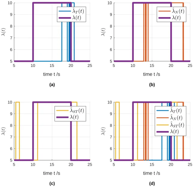
for traffic drop [12]. 𝑛 is a discretized time index in the unit of arrivals. 61 3-7 The comparison of traffic surge/drop detections among different
esti-mators with 𝑝𝑚 = 1%. 𝑇 = 6.2 for ^𝜆𝑇(𝑡), 𝑁 = 43 for ^𝜆𝑁(𝑡), 𝜂− = 0.575
for ^𝜆𝑆𝑇(𝑡). Here it is already assumed the traffic rate jumps between
two states: (a) The fixed-time estimator ^𝜆𝑇(𝑡); (b) The fixed-count
estimator ^𝜆𝑁(𝑡); (c) The stopping-trial estimator ^𝜆𝑆𝑇(𝑡); (d) All three
estimators. 𝜋𝜆0 = 𝜋𝜆1 = 0.5, 𝜆0 = 5, 𝜆1 = 10. [59] . . . 64
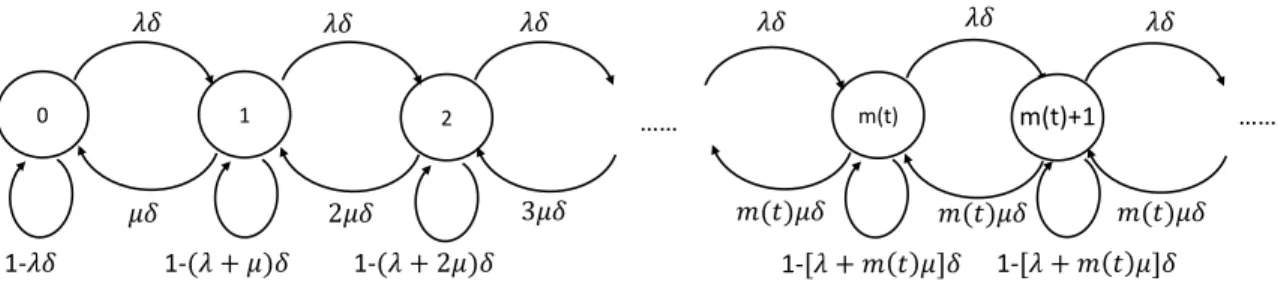
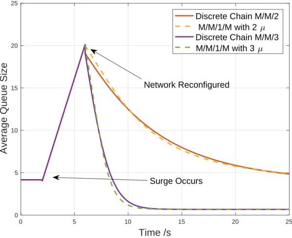
3-8 Sampled-time approximation to 𝑀/𝑀/𝑚(𝑡) queue with a very small time increment 𝛿. . . 66 3-9 (a) Simulated and analytical results of the evolution of queue size for a
network surge followed by a proper reconfiguration for an 𝑀/𝑀/1/𝑋 queue. 𝜋𝜆0 = 𝜋𝜆1 = 0.5, 𝜆0 = 5, 𝜆1 = 10, 𝜇 = 6.[59] . . . 71
3-10 The transient behavior of the average queue size when a surge occurs and a proper reconfiguration is made later. 𝜋𝜆0 = 𝜋𝜆1 = 0.5, 𝜆0 =
3-11 Transient behavior of the average queue size with only one reconfigu-ration for different detection times of the fixed-time estimator ^𝜆𝑇(𝑡).
𝜋𝜆0 = 𝜋𝜆1 = 0.5, 𝜆0 = 5, 𝜆1 = 10, 𝜇 = 6. . . 73
3-12 Transient behavior of the average queue size with multiple reconfigu-rations for different detection times of the fixed-time estimator ^𝜆𝑇(𝑡).
𝜋𝜆0 = 𝜋𝜆1 = 0.5, 𝜆0 = 5, 𝜆1 = 10, 𝜇 = 6. . . 74
3-13 Normalized average peak delays versus surge changes and detection times 𝜏1. 𝜋𝜆0 = 𝜋𝜆1 = 0.5, 𝜆0 = 5, 𝜇 = 6. [59] . . . 82
3-14 Average normalized queueing delay for different detection times 𝜏1with
one reconfiguration for different detection times of the fixed-time esti-mator ^𝜆𝑇(𝑡). The results are the average of both detections and false
alarms. 𝜋𝜆0 = 𝜋𝜆1 = 0.5, 𝜆0 = 5, 𝜆1 = 10, 𝜇 = 6.[59] . . . 83
3-15 Average normalized queueing delay for different detection times 𝜏1with
multiple reconfigurations for different detection times of the fixed-time estimator ^𝜆𝑇(𝑡). The results are the average of both detections and
false alarms. 𝜋𝜆0 = 𝜋𝜆1 = 0.5, 𝜆0 = 5, 𝜆1 = 10, 𝜇 = 6.[59] . . . 84
3-16 Cost transition versus time with one reconfiguration. The results are the average of both detections and false alarms. 𝜋𝜆0 = 𝜋𝜆1 = 0.5, 𝜆0 =
5, 𝜆1 = 10, 𝜇 = 6. 𝐶𝑤 = 𝐶𝑑 = 100, 𝑝𝑚 = 10%. [59] . . . 86
3-17 Cost transition versus time with multiple reconfigurations. The results are the average of both detections and false alarms. 𝜋𝜆0 = 𝜋𝜆1 =
0.5, 𝜆0 = 5, 𝜆1 = 10, 𝜇 = 6. 𝐶𝑤 = 𝐶𝑑= 100, 𝑝𝑚 = 10%. [59] . . . 87
3-18 Cost comparison of different estimators with 𝑝𝑚 = 10%. 𝜋𝜆0 = 𝜋𝜆1 =
0.5, 𝜆0 = 5, 𝜆1 = 10, 𝜇 = 6. 𝐶𝑤 = 𝐶𝑑= 100. [59] . . . 88
3-19 Optimal number of wavelengths comparison versus cost parameter ra-tio 𝐶𝑤/𝐶𝑑of different estimators. 𝜋𝜆0 = 𝜋𝜆1 = 0.5, 𝜆0 = 5, 𝜆1 = 10, 𝜇 =
6. 𝐶𝑤 = 𝐶𝑑= 100, 𝑤0 = 1, 𝑝𝑚 = 10%. [59] . . . 90
3-20 Optimal number of wavelengths comparison versus load 𝜌 of different estimators. 𝜋𝜆0 = 𝜋𝜆1 = 0.5, 𝜆0 = 5, 𝜆1 = 10, 𝜇 = 6. 𝐶𝑤 = 𝐶𝑑 = 100,
4-1 The threshold trigger processes with different counting start points. [60] . . . 96 4-2 The comparison of simulated wavelength assignment of ^𝜆𝑆𝑇(𝑡) and
the desired wavelength assignment in different network traffic envi-ronments: (a) long network coherence time; (b) moderate network coherence time; (c) short network coherence time. [60] . . . 98 4-3 The range of the average detection time 𝜏1 of ^𝜆𝑆𝑇(𝑡) versus
probabil-ity of missed detection (crossing thresholds) for different arrival rate ranges. [60] . . . 102 5-1 Analytical upper bounds and numerical results on the settling time
𝜏2 versus different distances between the initial steady-state
proba-bility distribution and the new steady-state probaproba-bility distribution after the network drift with different convergent rates (the second largest eigenvalue in magnitude of the probability transition matrix). 𝑙 = 100, 𝑎𝑖,𝑖+1 = 10 (0 < 𝑖 < 𝑙 − 1), 𝛿 = 0.01𝑠, 𝜖 = 10−5. [60] . . . 113
5-2 Slope estimation of the network traffic drifting trend in a linear in-creasing model versus different number of arrivals over 200 runs. The probability distribution of the arrivals is the same but each time the arrival samples will be randomly generated. Λ𝑜 = 5, 𝑘 = 0.2. [60] . . 119
6-1 The Petersen graph with several secondary paths for rerouting between node pair 𝐴 − 𝐵 with 1-hop primary path. . . 124 6-2 Secondary paths for rerouting for the Petersen graph. (a) All the 4-hop
paths; (b) All the 5-hop paths. . . 126 6-3 Conditional blocking probabilities of different secondary paths on the
Petersen graph for the node pair 𝐴 − 𝐵 with 1-hop primary path. The blocking on each hop is assumed to be statistically independent of each other. . . 127 6-4 Secondary paths for rerouting for two extreme five-node topologies. (a)
6-5 Path blocking probability versus the blocking probability on a hop for different topologies. The blocking on each hop is assumed to be statistically independent with each other. . . 130 6-6 The traffic supporting ratio versus percentage of reserved wavelength
for a 10-node network topology. The shortest-path algorithm is adopted to find the secondary path for rerouting and only the shortest secondary paths are used. . . 134 6-7 The expected number of transactions in the holder when the
thresh-old is crossed 𝐸[𝐾] versus the queueing delay threshthresh-old 𝜏𝑄𝑇 ℎ𝑟𝑒𝑠ℎ. for
different traffic situations. The wavelength number is 1 per node pair. A unit delay is defined as the transmission delay of a mouse traffic transaction. The transmission delay of an elephant traffic transaction is 106 units of delay. . . 139 6-8 The expected number of transactions in the holder when the threshold
is crossed 𝐸[𝐾] versus the number of wavelengths assigned between each node pair for different traffic situations. A unit delay is defined as the transmission delay of a mouse traffic transaction. The transmission delay of elephant traffic is 106 units of delay. 𝜏
𝑄𝑇 ℎ𝑟𝑒𝑠ℎ. = 10
List of Tables
6.1 Table of secondary paths for rerouting for the node pair A to B in a Petersen graph. . . 125
Chapter 1
Introduction
The dynamic large traffic generated by diverse technology applications will drive the architecture of future optical networks. The bursty, unscheduled, and large data transactions introduced by new technological applications can cause both high costs and extreme congestions in networks. In the current quasi-statically configured net-work, lack of over-provisioning will manifest as huge congestions during peak demand periods. The dynamic and bursty (unpredictable) nature of large traffic transactions either requires over-provisioning of the networks, which is costly, or a more agile network control and management system that adaptively allocates resources by re-configuring the network in a timely manner in reaction to the offered traffic. The network management and control system should be able to sense traffic changes and make reconfigurations to use network resources efficiently. Specifically, reconfigura-tions should be done on a subsecond time scale with no human involvement. To meet these demands, cognitive networking is proposed as a candidate architectural construct that can provide fast, dynamic, and efficient control using cognitive tech-niques.
1.1
Increasing Traffic
Emerging network applications will make the offered traffic in future optical networks more bursty with high granularity sessions from megabytes to terabytes. The high
granularity indicates the increased volume of large traffic. Compared to the past when major traffic is only in the range of bits to megabytes, now much larger traffic occurs in gigabytes or even in terabytes. Within five to ten years, current optical networks are predicted to have an approximately three to four orders of magnitude increase in data rates, mostly due to large transactions. It is reported in [16] that IP video traffic will be 82% of all IP traffic (both business and consumer) by 2022 globally. As indicated in [15], an Internet-enabled High-Definition (HD) television that draws two to three hours of content per day from the Internet would generate a similar amount of traffic on average as the Internet traffic generated by an entire household today. Moreover, the increasing demands of Ultra-High-Definition (UHD) with 4K or even 8K video streaming will have more profound effects on the traffic growth due to the increase in the bit rate. The bit rate for 4K video is about 15 to 18 Mbps, which is more than double the HD video bit rate and nine times more than the bit rate of Standard-Definition (SD) video [15]. It is estimated in [15] that two-thirds of the installed flat-panel TV sets will be UHD by 2023, up from 33% in 2018. Besides, various new devices and new applications make the traffic patterns more diverse. Among them, Machine-to-Machine (M2M) applications are the major contributors, such as video surveillance, healthcare monitoring, smart meters, transportation, package or asset tracking, etc [15]. It is predicted in [15] that M2M connections will be half of the total devices and connections by 2023. All the dynamic large traffic generated by the diversity of technology applications will drive the architecture of future optical networks.
The extreme burstiness and high granularity of the network traffic is challenging today’s optical networks, as it requires optical network control to be much more dy-namic unless expensive large over-provisioning is used. Due to the dydy-namic traffic, statistical multiplexing to smooth quiescent flows between major nodes will not occur most of the time. The highly complex and dynamic networking environments will pose serious challenges for physical and higher network layers architecture, and greatly in-crease the network operating costs. The current network management and control systems of the backbone optical networking is much too slow to handle the variety
of traffic that comes from modern integrated global heterogenous networks, which include but are not limited to wireless networks, satellites networks, etc. It is because the current architectures of optical networks were designed for the quasi-static sta-tistically multiplexed traffic of the past. Even for current software-defined-networks (SDN), network function virtualization (NFV), and orchestration, their network re-configuration times range from tens of minutes to hours and even to days, which are inadequate to deal with current second-scale traffic changes [44]. The backbone opti-cal networking needs to support different infrastructures from many access networks for millions of mobile users, and various traditional and new network services, such as data centers/private clouds [23], Software as a Service (SaaS), Infrastructure as a Service(IaaS), Internet-of-Things(IoT) [1], video-based searches [22], etc.
The increasing dynamic and high-granularity traffic will require a much smarter network management and control system to rapidly adapt to bursty applications and their service needs, especially for the increasingly large-volumed “elephants”. Un-predictable dynamic traffic changes require quick network adaptation on a scale of seconds to maintain users’ quality of service, such as the service delay. Moreover, service-based architecture requires dynamically tailored network configurations. In the near term (2020), we expect an active control plane in minutes for network orches-tration [44], such as dynamic load balancing. In the mid term (2021+), a very active control plane is expected with functions including agile access points, per-session routing (segment routing), and the Internet of Things(IoT)/smart-city applications [1]. In the far term(2023+), we expect more dynamic network functions such as mid-session rerouting, etc. The control planes are designed for time critical services and network security and safety[12]. Network adaptions are expected to be performed on a scale of a second (∼ 100 milliseconds - 1 second). Therefore, efforts should be made to develop a new optical network control and management scheme that can quickly sense the network and reconfigure within a much shorter amount of time than before, preferably as quickly as statistically viable. The new scheme should reduce human involvement, since humans in the loop of current networks contribute to the most reconfiguration time and control costs. Meanwhile, the network control and
man-agement system should be kept simple and efficient enough to reduce the burdens of network operations.
1.2
Cognitive Optical Networking
Cognitive networking is a desirable architecture construct that can provide fast, dy-namic, and efficient control using automated cognitive techniques to meet the above requirements. As defined in [45][46], a cognitive network can sense current network conditions, and then autonomously learn and make decisions from these conditions to realize end-to-end goals. Its cognitive control and management scheme can respond to network changes and reconfigure the networks in a short amount of time without tedious network tuning by humans. For current network architectures, the intrinsic system complexity will increase explosively in the near future, but the current prac-tice has a limit that makes such increase computationally intractable and expensive. When intelligence is introduced, the operational complexity will come down. In short, intelligence enables the adaptive network to scale. The goal of cognitive networking is ultimately fully automated networks without any human involvement [45][46].
The exploration of cognitive techniques on optical networks started only a decade ago. The idea of incorporating cognitive techniques into networks was originally intro-duced to wireless systems and networks to solve the spectrum sensing and allocation problem in the 2000s [45] [35], such as the idea of cognitive radios. The idea of using a large amount of information gained from the experience of network nodes to im-prove the overall network and user performance is proposed in [34]. Increasingly, the idea of cognitive networks is growing beyond the use of cognitive radios to improve the performance of heterogeneous networks. The exploration of the use of cognitive techniques in the domain of optical networks started around 2010. However, most researchers have focused on using cognitive techniques to solve specific optical net-work operating problems, and the design of comprehensive cognitive optical netnet-work control and management schemes are still conceptual [53, 52, 48, 36, 19, 20, 43, 42, 6]. Several groups of researchers have proposed the designs of general cognitive
con-trol and management schemes for optical networks, but these ideas are still far from practical implementation. Zervas and Simeonidou have briefly provided a prototypical distributed cognitive architecture called COGNITION [53, 52]. Cognition is expected to be implemented from the bottom physical layer to the top application layer of the network architecture across one or multiple domains. However, more implementation details and verifications are needed, especially on the complicated network manage-ment and control plane. Wei et al. have proposed a cognitive optical substrate with a mesh topology only in the core networks. This substrate aims to provide high-speed, bandwidth-on-demand and rapidly-adaptive wavelength services in a client-service-aware approach [48]. However, the design of the substrate concerns only the physical layer and has no coordination with higher-layer functionalities. The project Cognitive Heterogeneous Reconfigurable Optical Networks (CHRON) has been pro-posed by several groups of researchers in Europe [14] to improve the dynamicity of the optical network control planes. The project has investigated in the intelligent monitoring techniques, the cross-layer cognitive control architecture design, and the multi-objective optimization of the performance in term of cost and energy efficiency [14]. Monroy et al. have designed a network control plane architecture in CHRON [36, 19]. The control plane of CHRON includes a cognitive decision system and a network monitoring system. Later, de Miguel et al. have successively elaborated the centralized cognitive framework and built a testbed [20, 43, 42, 6]. However, their design has not comprehensively solved the efficient network monitoring problem or the fast reconfiguration problem. Moreover, the four-node network topology in their testbed is too simple to validate the performance of the design in real-life networks, which usually have hundreds of nodes. In particular, there is no work that shows that reconfiguration can be done based on observed traffic changes. In summary, a comprehensive cognitive network management and control scheme for current optical networks is needed.
Chan et al. have proposed a detailed cognitive all-optical network architecture in [10, 9, 12]. Figure 1-1 shows the concept of the cognitive all-optical network with optical gateways between hierarchical subnet, peering gateway control points, and
Vincent Chan Claude E. Shannon Communication and Network Group, Research Laboratory of Electronics 6
isolation, reconstitution, re-optimization, insertion of key interconnects, …
Figure 1-1: Cognitive all-optical network concept with optical gateways between hi-erarchical subnet, peering gateway control points and cognitive engine sensing and interacting with multiple layers for network control. Reproduced from [7, 9].
cognitive engine sensing and interacting with multiple layers for network control from the works in [7, 9]. The cognitive engine senses and interacts with multiple layers to perform the dynamic control of the whole network system, such as the scalable fault management with dynamic probing of the network states in [50], the fast scheduling algorithm with a probing approach to enable the setup of end-to-end connections [54]. It may reside at network nodes as well as at a centralized or distributed controller/s. Figure 1-2 further elaborates a desired development of agile, responsive, and affordable on-demand network services via new network management and control architecture across all network layers from Layer 1 Physical Layer to Layer 7 Application Layer [8] [10]. The cognitive network management and control architecture will incorporate with the upgraded physical layer to support big and bursty “elephant” traffic [55, 56]. The major technology advances in physical layer include the massive integration via silicon photonics and hybrids for reduction in footprints (increasing density) lower costs, weight, and power consumption [55]. A dynamic transport layer protocol and data center routing topology and partitioning of resources is required as shown in [26].
A cognitive network management and control system can sense the current network state conditions, such as traffic and flow patterns, and uses this information to decide how to adapt the network to satisfy or improve overall performance and provide quick responses to transaction requests [7, 9]. The cognitive network module is part of the control plane that touches all layers of a network. Traditionally, users never interact with the control plane [55, 56]. In the future optical network, users can interact via Application Layer or Transport Layer, and off-band control network. Interactions necessitated by sudden traffic changes of elephant traffic require fast adaptations.
Vincent Chan Claude E. Shannon Communication and Network Group, Research Laboratory of Electronics Vincent Chan Claude E. Shannon Communication and Network Group, Research Laboratory of Electronics
End-to-end reliability
Routing, wavelength assignment, congestion control, fairness Framing, error correction Media Access Control (MAC) User/network API User Network DLC Application Presentation Session Transport Network Data link control Physical Application Presentation Session Transport Network Data link control Physical Physical Physical Physical Physical
DLC DLC DLC
Network Network
Virtual network service Virtual session Virtual link for end to end messages
Virtual link for end to end packets
Virtual link for reliable packets Virtual bit pipe
Physical link
External site Subnet node Subnet node External site
L-7 L-6 L-5 L-4 L-3 L-2 L-1 N et w or k M ana g em ent a nd C ont rol P la ne
User interaction via Application Layer or Transport Layer off-band control network or via separate heart beat network
6
Cognitive engine as part of control plane
Figure 1-2: An agile control plane architecture of cognitive network management and control system. Reproduced from [8, 10].
In summary, the desired new network management and control architecture in cognitive optical networking should have the following features:
1. Inference of network states based on traffic and active probing often with sparse and stale data [50, 54];
2. All-optically switched architecture that provides agility and efficient resource usage [11, 55];
3. Decisions and actions taken on load balancing, reconfiguration, restoration [50, 55];
4. Cognitive techniques that predict optimum configuration for fast adaptation to improves network performance without detailed assumptions of channel and traffic statistics [31, 10].
The first point is discussed in [38, 40] with the design of the cognitive significant state sampling for a cost-effective network management system. It is shown in [38] that the adaptive monitoring system can greatly reduce the network management and control overhead if the network states information is only collected when it can improve network performance. The second point is discussed in [11, 49, 24, 27, 28, 55, 56, 57] with the comprehensive design of Optical Flow Switching (OFS). OFS is an agile all-optical end-to-end network service for users with large traffic flows that bypass routers. The dynamic per flow on a time scale of 1−104 seconds scheduling can
prevent collisions, and off-band signaling is used for reservation, scheduling, and setup on a time scale of < 100 milliseconds. The fourth point is mentioned in [31, 10], where the cognitive method for routing with the potential for improvements in network performance is discussed. In [31], the inference and estimation methods are used on the network traffic to modify the parameters of their routing protocols and/or routing tables to improve performance metrics such as packet delay or network throughput.
In this work, we will mainly focus on the third and fourth points as our design goals to enable cognitive optical networking control and management to be done in a timely manner. We will try to optimize network configurations to improve network performance based on the traffic information.
1.3
Design Goals
The goal of this work is to provide insights into the design of a comprehensive and practical cognitive control and management scheme for optical networks. Specifically, the design should provide an efficient and simple way to implement architectures that can avoid a big burden for network management and control, and to improve the cost efficiency of dynamic large transactions.
maintain a low queueing delay with the fastest possible algorithms (and that means no human in the loop). This is extremely important for the network in terms of stability, scalability, reliability, and evolvability. It not only guarantees that optical networks can function well in the traffic with great granularity, but it has to be scalable when the network grows larger and faster. With the fast dynamics noted, agile cognitive optical network management and control systems will guarantee both the quality of transmission and network robustness with little or no involvement of humans, and will finally move towards intelligent automatic control of networks. All of these make it more affordable to meet changing requirements and incorporate new technology as the network evolves.
Based on the design goal mentioned above, this work will mainly focus on two modules to enable cognitive optical networking control and management in a timely manner with little or no human involvement as:
1. Traffic detection and estimation – fast recognition of the nonstation-ary traffic changes;
2. Network reconfiguration – quick adaption based on input quality of service metric (delay, cost, etc.) and optimum sequential decision algorithm.
The traffic detection and estimation module focuses on an efficient way to detect and estimate the network traffic state information for sequential accurate network reconfiguration. Traditional approaches to traffic change detection and estimation require the collection of excessive historical network traffic information to allow for fast and agile reconfiguration of network resources. The prevalence of dynamic traffic sessions in today’s networks, which manifest themselves through frequent and bursty changes of the network states, makes such approaches ineffective and even infeasible sometimes. Therefore, we need to design a traffic detection and estimation scheme that can make a decision in the shortest possible time when the traffic statistics provide enough confidence for reconfiguration to enhance the ability of the network to respond to changes efficiently.
The network reconfiguration module focuses on accurately adapting the network configurations based on the current operating conditions. In this work, three major reconfiguration options are used in order of preference for the reconfigurable network architecture are:
1. Lighting up a wavelength in the same primary lightpath between a node pair; 2. Rerouting incremental traffic to a secondary path with open wavelengths
be-tween the node pair;
3. Lighting up a new fiber with multiple wavelengths together with optical switch-ing to accommodate overflowswitch-ing traffic.
The reconfiguration can leverage the historical data as well as the real-time infor-mation acquired from monitoring to guide the decision process. Accurate prediction of future network states based on past traffic as well as active probing algorithms are essential for any modern management protocol.
1.4
Cognitive Optical Network Design Submodules
We further break down the two general modules in the previous section into the fol-lowing submodules to guide the design of a fast-reconfigurable network. The core of cognition in networking is self-initiated actions. To be more specific, the networks are equipped with the capability to flexibly sense network conditions and then reconfigure dynamically. Also, network costs need to be considered to guarantee that architecture is affordable to be implemented widely. To complete this fast-reconfigurable and eco-nomical cognitive optical network architecture design, the following points of network management and control scheme needed to be stressed.
1. Define the dynamic network traffic environment. This section will focus on how to depict different network traffic environments.
2. Detect and estimate current network traffic fast and efficiently. This problem will focus on efficiently detecting current real-time traffic to gain information
about traffic shifts for network reconfigurations. To upgrade the cognitive control to the autonomous adaption to current and upcoming network conditions, a traffic estimation based on previous traffic detection results is desired.
3. Monitor the changes of queues when traffic or network reconfigura-tion changes. This problem will focus on depicting the transient behaviors of the queues in the networks to gain an understanding of how the fast network changes affect the whole systems on a real-time scale.
4. Design the efficient network reconfiguration scheme. With given traf-fic information and network state information (NSI), the network can reconfigure to improve network performances and save operating costs. Adjustment include both network setting changes (wavelength changes, etc.) and dynamic traffic controls (net-work load balancing, traffic congestion control, etc.). Continuous assessments on de-cisions and network controls will be an attribute of the scheme to provide the dynamic optimization of network performance.
5. Evaluate the performance of cognitive design. Questions to be solved include what performance metrics are used and how the cognitive algorithms perform. 6. Estimate the cost of the architecture. Cost evaluations of the network in terms of both capital expenditure (e.g., wavelengths) and operating expenditure (e.g., queueing delay) should be given. Also, recommendations on how to further reduce control complexity should be given.
The architectural recommendation provided in this work will cover all six points above.
1.5
Thesis Scope and Organization
The rest of the thesis is organized as follows.
In Chapter 2, we discuss the traffic model that captures the dynamic traffic en-vironment, the tunneled network architecture, and the reconfiguration options. We build a traffic model based on the characteristics of the dynamic, bursty, and high-granularity traffic. The tunneled network architecture is adopted due to its supremacy
in reducing the control complexity. Three major reconfiguration options in order of preference for the reconfigurable network architecture are introduced.
In Chapter 3, we develop the design of fast-reconfigurable cognitive wavelength management and control algorithms that can accurately adapt based on the traffic conditions in the long coherence time environment, where the traffic changes very slowly. We develop two Bayesian estimators and a stopping-trial estimator to detect traffic changes. We model the transient behaviors of networks to evaluate the detec-tion and queueing delay performances of different estimators. A network cost model is also proposed to stress the trade-off between queueing delay performance and the cost of the capacity plus the control resources used. Finally, the stopping-trial esti-mator with continuous assessment is recommended due to the fastest response time to traffic changes following by the lowest operating cost.
In Chapter 4, we discuss the fast detection in the moderate coherence time envi-ronment, where the traffic changes at a moderate rate. We validate the efficacy of the stopping-trial estimator and discuss its detection performance. As long as the inter-arrival times of traffic sessions are independent but not necessarily identically distributed, the stopping-trial estimator is still recommended as it can react effectively to the traffic rate changes.
In Chapter 5, we discuss traffic trend detection in the short coherence time en-vironment, where the traffic changes very quickly. We model the transient behavior of the network traffic as it drifts towards convergence at a new steady state and val-idate the feasibility of the traffic trend prediction. Given the fast-changing traffic where the traffic rate changes monotonically in a linear model, we develop the de-sign of predicting the traffic trend with a sequential maximum likelihood estimator based on distribution of the inhomogeneous Poisson process. The algorithm can suf-ficiently estimate the traffic trend with a reasonable number of arrivals and trigger reconfigurations.
In Chapter 6, we discuss the rerouting algorithm. We develop the rerouting al-gorithm implemented with the shortest-path alal-gorithm. The rerouting is triggered by a threshold on the queueing delay, and the threshold is directly determined by
the current traffic situation and the network configurations. We also discuss the op-tion to reserve wavelength for rerouted traffic only and do not recommend it due to low resource utilization. The desired properties of paths for rerouting and network topology are discussed. Traffic splitting with resources partitioned in rerouting is recommended for better network utilization.
In Chapter 7, we conclude the thesis with a summary of the recommended archi-tectural design of the cognitive optical networks in the dynamic traffic environments. We also present some directions for future work.
Chapter 2
Dynamic Traffic Environment,
Tunneled Architecture, and
Reconfigurations
In this chapter, we discuss the simplified traffic model that captures the dynamic traf-fic environment, the tunneled network architecture, and the reconfiguration options. We build a simplified traffic model to reflect the characteristics of dynamic, bursty, and high-granularity traffic. The tunneled network architecture will be adopted due to its supremacy in reducing the control complexity [55]. In the following chapter, we design the detection and reconfiguration scheme to fulfill the traffic demands based on this traffic model presented in this chapter.
2.1
Dynamic Traffic Model
One of the main contributions of this work is to build a model of the time-varying stochastic traffic in the optical networks, which is usually ignored in the static or quasi-static traffic model in previous work. Other traffic models depicting the time-varying stochastic traffic can be discussed in future work. To capture the bursty nature of traffic, we address the different changes in it. Traffic environments can be categorized into three regimes as follows:
1. Network traffic changes very slowly so adaption can be done while the traffic is in the same state;
2. Network traffic changes at a moderate rate commensurate with the fastest adap-tion times;
3. Network traffic changes very rapidly so adaptions can only be limited to trends rather than to the detailed changes.
A comprehensive analysis of such dynamic network environments is a must for the design of cognitive management and control of optical networks. In the following chapters, we focus on the design of a traffic detection mechanism and the reconfigu-ration scheme for all three regimes.
2.1.1
All-to-all Stochastic Traffic
Given a network in the topology form, each node sends a certain amount of traffic to other nodes for transmission. For a well-planned network, the average traffic should be balanced to maintain a low network operating cost [24]. For example, in a Metropolitan Area Network (MAN), the average traffic volume generated in each MAN node should be approximately the same because the network resources are partitioned based on the traffic demands. Several areas with low traffic demands will share the same MAN node, while an area with high traffic demands will be allocated an entire MAN node [24, 58]. Besides, traffic transmission among different node pairs should be considered as statistically independent, since traffic is aggregated from different areas.
In the traffic model, we assume that every source-destination node pair has uni-form all-to-all independent and identically distributed (I.I.D.) traffic as shown in Fig. 2-1. The I.I.D. property applies to both the traffic arrival pattern and the traffic trans-action size. The I.I.D. arrival pattern comes from the evenly balanced traffic among all the nodes. The I.I.D. traffic transaction size is adopted to facilitate analyses.
Figure 2-1: All-to-all dynamic traffic.
2.1.2
Multi-state Markov Arrival Rate
The traffic arrivals between each source-destination pair is assumed to follow a doubly stochastic point process with a changing arrival rate 𝜆(𝑡). Compared to a fixed arrival rate, the current model with a changing rate can not only cover a wider range of arrival patterns, but capture the burstiness of the traffic. Though the detection and estimation of the changing arrival rate are much harder than the unvarying arrival rate, our model with the changing arrival rate will provide a more generic solution.
We can describe the Poisson arrival process of the traffic in two ways. First, we describe the number of arrivals 𝑁 in the observation interval. 𝑁 follows a Poisson distribution with the rate of 𝜆(𝑡)𝑇 . By counting the number of arrivals in the ob-servation time, we can estimate the arrival rate. Denote the obob-servation interval as [𝑡 − 𝑇, 𝑡] with the length of 𝑇 . To avoid ambiguity, we include both the epochs (𝑡 − 𝑇 ) and 𝑡. The number of arrivals in the interval [𝑡 − 𝑇, 𝑡] is denoted as 𝑁 (𝑇 ) and we have
𝑃 𝑟[𝑁 (𝑇 ) = 𝑛] = (𝜆(𝑡)𝑇 )
𝑛𝑒−𝜆(𝑡)𝑇
𝑛! . (2.1)
𝐸[𝑁 (𝑇 )] = 𝜆(𝑡)𝑇. (2.2)
The variance of the number of arrivals in the observation time 𝑇 is
𝑉 𝑎𝑟[𝑁 (𝑇 )] = 𝜆(𝑡)𝑇. (2.3)
Second, we can describe the length of the inter-arrival time and further the total length time of 𝑁 arrivals. Each inter-arrival time in {𝑇𝑖, 𝑖 ≥ 1} follows an exponential
distribution with parameter 𝜆(𝑡). We assume the first arrival always happens at the starting time (𝑡 − 𝑇 ), and 𝑇𝑖 is the inter-arrival time between the 𝑖𝑡ℎ arrival and the
(𝑖 + 1)𝑡ℎ arrival. The sum of 𝑁 inter-arrival times 𝑇 (𝑁 ) =∑︀𝑁
𝑖=1𝑇𝑖 follows an Erlang
distribution with 𝜆(𝑡) as
𝑃 𝑟[𝑇 (𝑁 ) = 𝜏 ] = 𝜆(𝑡)
𝑁𝜏𝑁 −1𝑒−𝜆(𝑡)𝜏
(𝑁 − 1)! . (2.4)
The expectation of the observation length with 𝑁 number of arrivals in the ob-servation time 𝑇 is
𝐸[𝑇 (𝑁 )] = 𝑁
𝜆(𝑡). (2.5)
The variance of the observation length with 𝑁 number of arrivals in the observa-tion time 𝑇 is
𝑉 𝑎𝑟[𝑇 (𝑁 )] = 𝑁
We assume 𝜆(𝑡) follows a Markov process, where the traffic arrival rate 𝜆(𝑡) switches among different states 𝜆1, 𝜆2, ..., 𝜆𝑙 as the embedded Markov chain of a
countable-state Markov process shown in Fig. 2-2, where 0 < 𝜆1 < 𝜆2 < ... < 𝜆𝑙. In
this model, the traffic arrival rate will not change dramatically in a short amount of time. We assume the transitions only include a state that switches to its previous state, its next state, or itself. The transition from 𝜆𝑖 to 𝜆𝑖+1(0 < 𝑖 < 𝑙 − 1) indicates a
traffic surge, and we want to detect it promptly to avoid potential traffic congestion and large queueing delays. The transition from 𝜆𝑖+1 to 𝜆𝑖, (0 < 𝑖 < 𝑙 − 1) indicates a
traffic drop, and we also want to detect it promptly to avoid any waste of resources. When 𝜆(𝑡) is maintained at state 𝜆𝑖, there is no traffic change, and we assume the
holding interval associated with the state 𝜆𝑖 follows an exponential distribution with
a rate of 𝑣𝑖, which is called as the holding rate. Each state is associated with a
transition rate 𝑎𝑖,𝑗 from 𝜆𝑖 to 𝜆𝑗.
𝜆" 𝜆# 𝜆$%"
𝑎
",#𝑎
#,(𝑎
$%#,$%"𝑎
$%",$……
𝑎
#," 𝜆$𝑎
(,#𝑎
$%",$%#𝑎
$,$%"Figure 2-2: Multi-state embedded Markov chain transition of the traffic arrival rate 𝜆(𝑡).
Later in Chapter 3, we will simplify the model and assume the traffic switch between a non-surging state 𝜆0 and a surging state 𝜆1 to focus on the detection
2.1.3
Network Coherence Time
In this work, we model the network coherence time as the holding interval where the traffic arrival rate is maintained at a certain state, and we denote the average coherence time as 𝐷𝑖. The average coherence time of the whole system is denoted as
𝐷. In our traffic arrival model, given the current state is 𝜆𝑖, the average coherence
time in state 𝜆𝑖 is 𝐷𝑖 = 1 𝑣𝑖 = 1 𝑎𝑖,𝑖−1+ 𝑎𝑖,𝑖+1 . (2.7)
It is because the network will remain in this state, and the time to the next transition is the time until either a transition to the previous state or the next state. With the steady state probability of state 𝜆𝑖 as 𝜋𝑖, the average coherence time for the
whole system is 𝐷 = 𝑙 ∑︁ 𝑖=1 𝜋𝑖 𝑣𝑖 . (2.8)
We can categorize the network traffic environments using the coherence time 𝐷 and the time to make decisions into three regimes. Denote the average detection time of the estimator as 𝜏1. The three regimes of the changing traffic represented in the
relation between the detection and the coherence time are:
1. long coherence time: 𝜏1 << 𝐷, where the traffic changes very slowly;
2. moderate coherence time: 𝜏1 ∼ 𝐷, where the traffic changes at a moderate rate;
3. short coherence time: 𝜏1 >> 𝐷, where the traffic changes very quickly.
Alternatively, we can quantize the coherence time with the holding rate 𝑣𝑖. We
assume 𝑣𝑖 is changing within a range of [𝑣𝑚𝑖𝑛, 𝑣𝑚𝑎𝑥]. The range of 𝑣𝑖 can be learned
and determined from the historical records of network traffic. The three regimes become:
1. long coherence time, where 𝑣𝑖 ∼ 𝑣𝑚𝑖𝑛;
2. moderate coherence time, where 𝑣𝑖 ∼ 𝑣𝑚𝑖𝑛+𝑣2 𝑚𝑎𝑥;
3. short coherence time, where 𝑣𝑖 ∼ 𝑣𝑚𝑎𝑥.
In the long coherence time regime, the inter-arrival times 𝑇𝑖s after the traffic
change are a set of I.I.D. variables and the I.I.D. property can facilitate the detection and the estimation of the traffic change. In the moderate coherence time regime, 𝑇𝑖s
are no longer identically distributed and this makes detection difficult. What is more, the traffic can change again. In the short coherence time regime, it is hard to detect every single traffic change. If the coherence time is extremely short, the detection may no longer converge. In this case, we can only try to predict the trend of fast traffic changes when the session arrival statistics provide enough confidence to do so.
2.2
Tunneled Architecture
We assume a tunneled network architecture, where each node pair is connected via a preselected set of wavelengths within a single lightpath or multiple lightpaths for traffic transmission as shown in Fig. 2-3. Zhang showed in [55] that tunneled archi-tecture can reduce control plane traffic and processing complexity significantly with little sacrifice in efficiency for heavy traffic volumes, compared to meshed architecture that enables full switchability at all nodes. The capacity between each node pair is reconfigurable by adjusting the number of wavelengths used by the node pair based on the offered traffic.
Assume 𝑚(𝑡) wavelengths are assigned between a node pair at time 𝑡, and each wavelength has a constant transmission rate of 𝑅 bits per second. The size of each transaction 𝐿 is assumed to be exponentially distributed with the expectation 𝐿0
in the analysis, but any well-behaved real-life traffic distribution will yield the same architecture recommendations. Given the average size of a transaction 𝐿0, the service
rate of each wavelength per transaction is 𝜇 = 𝐿𝑅
2 3 𝒎(𝒕) 1 …
S
D
All-to-all tunneled network topology
S
D
Reconfigurable wavelength assignment
(a)
(b)
Figure 2-3: An example of an all-to-all tunneled network connection between node pairs in the form of wavelengths. (a) All-to-all tunneled network topology; (b) Re-configurable wavelength assignment.
2.3
Traffic Load
We employ the traffic load to evaluate the traffic situation in the network. For a node pair, given the arrival rate 𝜆(𝑡) and the traffic service 𝜇 with 𝑚(𝑡) wavelength tunneled in use, we can define the network load between a node pair as
𝜌 = 𝜆(𝑡)
𝑚(𝑡)𝜇. (2.9)
The traffic load of the whole network can be reflected by the load on each node pair. The load of the whole network is the total arrival rate entering the network divided by the total transmission rate of all the wavelengths in use in the network. Given the uniform all-to-all traffic pattern, the average arrival rate of each node pair is the same, and the same number of wavelengths will be assigned to each node pair. Therefore, the average load of the whole network is the same as the average load on
each node pair.
The arrival and transmission between the node pair is in a stable state when 𝜌 < 1. When 𝜌 ≥ 1, the network is overloaded, and the queue between the node pair will grow. Network reconfigurations are needed to bring the system to a new steady state. Otherwise, either long delays or excessive blocking will degrade users’ quality of service.
2.4
Reconfigurations
When network traffic changes happen, network reconfigurations may be needed to maintain users’ quality of service. An agile network reconfiguration scheme is re-quired to accurately adapt based on the current operating conditions and maintain high cost efficiency. Any mismatch between network conditions and the suggested reconfigurations will increase network burdens and waste network resources.
It is not hard to see that the detection performance of the estimator will determine the following reconfiguration performance since fast detection can avoid the following severe network congestion. Also, high detection accuracy is required since high error probability makes the system unstable and degrades users’ quality of service. On the other hand, the network operating cost has to be taken into consideration to provide a reasonable reconfiguration scheme design.
Our goal is to provide timely network reconfigurations in response to the dynamic traffic environments. As discussed in Chapter 1, in the optical networks, with the traffic changes detected, three reconfiguration options in order of preference for the reconfigurable network architecture as shown in Fig. 2-4 are:
1. Lighting up a wavelength in the same primary lightpath between a node pair; 2. Rerouting incremental traffic to a secondary path with open wavelengths
be-tween the node pair;
3. Lighting up a new fiber with multiple wavelengths together with optical switch-ing to accommodate overflowswitch-ing traffic.
S D S D S D (a) (b) (c) S D Node Source Destination Fibers Route
Figure 2-4: The traffic transmission of three network reconfiguration options. (a) The dynamic wavelength addition or subtraction on the primary path. Traffic will be transmitted on the primary path. (b) The rerouting of the incremental traffic. Part of the traffic will be transmitted on paths other than the primary path. (c) The new fiber setup on the primary path. Traffic will be transmitted on the primary path.
The dynamic wavelength addition or subtraction is performed when the maxi-mum number of wavelengths on the path has not been reached. The traffic is still transmitted on the primary path between the source node and the destination node
as shown in Fig. 2-4(a). The fast-reconfigurable cognitive wavelength management and control algorithms aim to accurately adjust the number of assigned wavelengths based on the observation of the operating conditions of the networks. When traffic increases sharply, more wavelengths are expected to be assigned to avoid potential traffic congestion and large queueing delays. When traffic drops, fewer wavelengths are expected to avoid any waste of resources.
When the network traffic reaches a load threshold to satisfy delay requirements, the incremental traffic has to go through other paths to the destination, as shown in Fig. 2-4(b), which is called rerouting. In this work, it is performed when the queueing delay of the traffic transaction exceeds the delay requirement. If the overall system is heavily loaded, a new fiber with multiple wavelengths is needed to be set up, as shown in Fig. 2-4(c), which is equivalent to logically adding a path on the topology. This reconfiguration needs a longer cycle compared to the dynamic wavelength addition/subtraction. We will brief mention the time to perform fiber setup in Chapter 6.
Chapter 3
Long Coherence Time Traffic
Environment
In the long coherence time traffic environment, network traffic changes very slowly so adaption can be done while the traffic is in the same state. In other words, we have long enough time for detection and reconfigurations without worrying about more the traffic changes. For the detection of non-stationary traffic changes, we need to find the detection algorithm that can detect the network changes within the shortest possible time when the session arrival statistics provide enough confidence for reconfiguration. An optimal sequential estimator that can make a decision as soon as possible without any predetermined detection parameters is desired [12]. Also, the estimator should rely on less or no historical data and experience to be able to handle rare events effectively and efficiently [12]. This will remedy one of the blind spots of current learning techniques, where historical data is heavily relied on and unanticipated black-swan events are rarely recognized quickly and mitigated on time. The detection algorithm should quickly respond to unanticipated network situations and then avoid successive serious network catastrophes.
In this chapter, we present the design of fast-reconfigurable cognitive wavelength management and control algorithms that can accurately adapt by observing the net-work operating conditions of the netnet-works. Two Bayesian estimators and a stopping-trial estimator were proposed in [10, 12] to detect traffic changes. The Bayesian
estimator with the fixed observation time to classify the traffic state of the node is analyzed in [31]. Its average packet delay at a given node for various observation times is also given in [31]. In this work, we further develop these estimators and ex-amine their traffic detection and queueing delay performances based on the resulting transient behaviors of networks. A network cost model is proposed to capture the trade-off between reconfiguration performance (transient queueing delays) and the cost of the capacity plus the control resources used. We recommend a wavelength reconfiguration algorithm based on the stopping-trial estimator with continuous as-sessment where the system reconfigures whenever necessary. The reconfiguration can involve addition or subtraction of multiple wavelengths. Among the three estima-tors, the stopping-trial estimator requires the smallest number of wavelengths to be reconfigured because it responds the fastest and avoids a high peak queueing delay [59].
The arrival traffic at the source is assumed to form a doubly stochastic Poisson point process with a time-dependent rate of 𝜆(𝑡) as mentioned in Chapter 2. In [31], the traffic arrival model is assumed to transit between a surging state and a non-surging state. To facilitate the analysis in this chapter, we use a similar idea to assume 𝜆(𝑡) switches between a non-surging state 𝜆0 and a surging state 𝜆1, where 𝜆0 < 𝜆1
as shown in Fig.3-1. When 𝜆(𝑡) switches from 𝜆0 to 𝜆1, there is a traffic surge, and
we want to detect it promptly to avoid potential traffic congestion and large queueing delays. When 𝜆(𝑡) switches from 𝜆1 to 𝜆0, there is a traffic drop, and we want to
detect it promptly to avoid any waste of resources. The size of each transaction 𝐿 is exponentially distributed with the expectation 𝐿0 as defined in Chapter 2.
3.1
Two Bayesian Estimators
We first consider the commonly-used Bayesian estimators to detect the changes of traffic statistics. Given the binary nature of 𝜆(𝑡), two possible hypotheses for the decision are [31]:
𝜆
"𝜆
#𝑎
#,"𝑎
",#Surging
Non-surging
Figure 3-1: Two-state embedded Markov chain transition of the traffic arrival rate 𝜆(𝑡).
𝐻0 : 𝜆(𝑡) = 𝜆0; (3.1)
𝐻1 : 𝜆(𝑡) = 𝜆1. (3.2)
The false alarm probability 𝑃𝑓 is the probability that we accept 𝐻1 when 𝐻0 is
true. The missed detection probability 𝑃𝑚 is the probability that we accept 𝐻0 when
𝐻1 is true. The probability of detection is 𝑃𝑑= 1 − 𝑃𝑚. If the a priori probabilities
are known as 𝜋𝜆0 for 𝐻0 and 𝜋𝜆1 = 1 − 𝜋𝜆0 for 𝐻1, the total error probability is
𝑃 𝑟[𝑒] = 𝜋𝜆0𝑃 𝑟[𝐻1|𝐻0] + 𝜋𝜆1 (3.3)
= 𝑃 𝑟[𝐻0|𝐻1] = 𝜋𝜆0𝑃𝑓 + 𝜋𝜆1𝑃𝑚. (3.4)
We can observe the Poisson arrival process in two ways. First, we observe the number of arrivals 𝑁 in the observation interval [𝑡 − 𝑇, 𝑡]. 𝑁 follows a Poisson distribution with the rate of 𝜆(𝑡)𝑇 . Notice that 𝑇 should be less than the network coherence time for effective adaptions in the long coherence time traffic environment. Second, each inter-arrival time in {𝑇𝑖, 𝑖 ≥ 1} follows an exponential distribution with
parameter 𝜆(𝑡). As assumed in Chapter 2, the first arrival always happens at the starting time (𝑡 − 𝑇 ), and 𝑇𝑖 is the interarrival time between the 𝑖𝑡ℎ arrival and
the (𝑖 + 1)𝑡ℎ arrival. The sum of 𝑁 inter-arrival times ∑︀𝑁
𝑖=1𝑇𝑖 follows an Erlang
distribution with 𝜆(𝑡).
Given the two ways of observing the arrival process, we can develop two Bayesian estimators fixed-time estimator ^𝜆𝑇(𝑡) and fixed-count estimator ^𝜆𝑁(𝑡) as follows.
3.1.1
Fixed-Time Estimator ^
𝜆
𝑇(𝑡)
For the fixed-time estimator ^𝜆𝑇(𝑡), we count the total number of arrivals in a fixed
time interval [𝑡−𝑇, 𝑡] denoted by 𝑁 (𝑇 ) backwards in time to determine the validation of the hypotheses [12]. The observation window is moving with time. Here, 𝑁 is a random variable with the constant parameter 𝑇 . We define [12]
^ 𝜆𝑇(𝑡) =
𝑁 (𝑇 )
𝑇 . (3.5)
A similar analysis of the Bayesian estimator with the fixed observation time to classify the traffic state of the node with the arrivals in Poisson distribution as shown in [31].
Bayesian Likelihood Ratio Test
Similar to the Bayesian likelihood ratio test in [31], the Bayesian likelihood ratio test for 𝑁 (𝑇 ) with a priori probabilities 𝜋𝜆0 and 𝜋𝜆1 is
𝑃 𝑟[𝑁 (𝑇 ) = 𝑛|𝜆1] 𝑃 𝑟[𝑁 (𝑇 ) = 𝑛|𝜆0] 𝜆1 ≷ 𝜆0 𝜋𝜆0 𝜋𝜆1 , (3.6) where 𝑃 𝑟[𝑁 (𝑇 ) = 𝑛|𝜆0] = (𝜆0𝑇 ) 𝑛𝑒−𝜆0𝑇 𝑛! , 𝑃 𝑟[𝑁 (𝑇 ) = 𝑛|𝜆1] = (𝜆1𝑇 )𝑛𝑒−𝜆1𝑇 𝑛! . We get
⇔ 𝑛𝜆≷1 𝜆0 (𝜆1− 𝜆0)𝑇 + ln (︁𝜋 𝜆0 𝜋𝜆1 )︁ ln(︁𝜆1 𝜆0 )︁ , 𝛾𝑇. (3.7)
Therefore, we observe the number of arrivals 𝑁 (𝑇 ) in [𝑡 − 𝑇, 𝑡]. If 𝑁 (𝑇 ) ≥ 𝛾𝑇, we
accept 𝐻1 and reject 𝐻0. If 𝑁 (𝑇 ) < 𝛾𝑇, we accept 𝐻0 and reject 𝐻1.
Similar to the Bayesian likelihood ratio test in [31], when all the a priori proba-bilities are the same, i.e., 𝜋𝜆0 = 𝜋𝜆1 = 0.5, we have the test as
𝑛 𝜆1 ≷ 𝜆0 (𝜆1− 𝜆0)𝑇 ln(︁𝜆1 𝜆0 )︁ , 𝛾𝑇. (3.8)
The error probability 𝑃 𝑟[𝑒𝑇] for ^𝜆𝑇(𝑡) is
𝑃 𝑟[𝑒𝑇] = 𝜋𝜆0𝑃 𝑟[𝐻1|𝐻0] + 𝜋𝜆1𝑃 𝑟[𝐻0|𝐻1] (3.9) = 𝜋𝜆0𝑃 𝑟[𝑁 (𝑇 ) ≥ 𝛾𝑇|𝜆(𝑡) = 𝜆0] + 𝜋𝜆1𝑃 𝑟[𝑁 (𝑇 ) < 𝛾𝑇|𝜆(𝑡) = 𝜆1] (3.10) = 𝜋𝜆0 ∞ ∑︁ 𝑛=⌈𝛾𝑇⌉ 𝑃 𝑟[𝑁 (𝑇 ) = 𝑛|𝜆0] + 𝜋𝜆1 ⌈𝛾𝑇⌉−1 ∑︁ 𝑛=0 𝑃 𝑟[𝑁 (𝑇 ) = 𝑛|𝜆1] (3.11) = 𝜋𝜆0𝑒 −𝜆0𝑇 ∞ ∑︁ 𝑛=⌈𝛾𝑇⌉ (𝜆0𝑇 )𝑛 𝑛! + 𝜋𝜆1𝑒 −𝜆1𝑇 ⌈𝛾𝑇⌉−1 ∑︁ 𝑛=0 (𝜆1𝑇 )𝑛 𝑛! . (3.12) Neyman-Pearson Test
The Bayesian likelihood ratio test requires the knowledge of all the a priori prob-abilities. In practice, a more general case is that all the a priori probabilities are unknown. For the Neyman-Pearson test, it assumes all the a priori probabilities are unknown. As mentioned in [31], instead, define a threshold 𝜂 for the likelihood ratio test and we have
𝑃 𝑟[𝑁 (𝑇 ) = 𝑛|𝜆1] 𝑃 𝑟[𝑁 (𝑇 ) = 𝑛|𝜆0] 𝜆1 ≷ 𝜆0 𝜂, (3.13)
As mentioned in [31], similar to the expression in 3.7, the threshold expression is
𝑛 𝜆1 ≷ 𝜆0 (𝜆1− 𝜆0)𝑇 + ln 𝜂 ln(︁𝜆1 𝜆0 )︁ , 𝛾𝑇′. (3.14)
A Gaussian approximation to compute the error probabilities (and to create an ROC curve) instead of the exact error probabilities is shown in [31]. In this work, we prove the exact error probabilities as follows.
The type 1 error probability (false alarm probability) 𝑃𝑓𝑇 is the probability that we
accept 𝐻1but actually 𝐻0 is true, which is the same idea as 𝑃 𝑟[𝐻1|𝐻0] in the Bayesian
likelihood ratio test. Equivalently, it is the probability that we report 𝜆(𝑡) = 𝜆1 given
𝜆(𝑡) is actually in the level of 𝜆0. Since 𝑛 is an integer, we have
𝑃𝑓𝑇 = 𝑃 𝑟[𝐻1|𝐻0] = ∞ ∑︁ 𝑛=⌈𝛾𝑇𝑁⌉ 𝑃 𝑟[𝑁 (𝑇 ) = 𝑛|𝜆0] (3.15) = ∞ ∑︁ 𝑛=⌈𝛾𝑇 ′⌉ (𝜆0𝑇 )𝑛𝑒−𝜆0𝑇 𝑛! , (3.16)
where ⌈·⌉ is the ceiling function.
The type 2 error probability (missed detection probability) 𝑃𝑚𝑇 is the probability
that we accept 𝐻0 but actually 𝐻1 is true, which is the same idea as 𝑃 𝑟[𝐻0|𝐻1] in
the Bayesian likelihood ratio test. Equivalently, it is the probability that we report 𝜆(𝑡) = 𝜆0 given 𝜆(𝑡) is actually in the level of 𝜆1. Since 𝑛 is an integer, we have