HAL Id: hal-00876905
https://hal.archives-ouvertes.fr/hal-00876905
Submitted on 25 Oct 2013
HAL is a multi-disciplinary open access
archive for the deposit and dissemination of
sci-entific research documents, whether they are
pub-lished or not. The documents may come from
teaching and research institutions in France or
abroad, or from public or private research centers.
L’archive ouverte pluridisciplinaire HAL, est
destinée au dépôt et à la diffusion de documents
scientifiques de niveau recherche, publiés ou non,
émanant des établissements d’enseignement et de
recherche français ou étrangers, des laboratoires
publics ou privés.
Is the fish-hook effect in hydrocyclones a real
phenomenon?
Florent Bourgeois, Arun K. Majumder
To cite this version:
Florent Bourgeois, Arun K. Majumder. Is the fish-hook effect in hydrocyclones a real phenomenon?.
Powder Technology, Elsevier, 2013, vol.
237, pp.367-375.
�10.1016/j.powtec.2012.12.017�.
This is an author-deposited version published in :
http://oatao.univ-toulouse.fr/
Eprints ID : 9913
To link to this article : DOI:10.1016/j.powtec.2012.12.017
URL :
http://dx.doi.org/10.1016/j.powtec.2012.12.017
To cite this version :
Bourgeois, Florent and Majumder, Arun K.
Is the fish-hook effect
in hydrocyclones a real phenomenon?
(2013) Powder Technology,
vol. 237 . pp. 367-375. ISSN 0032-5910
Any correspondence concerning this service should be sent to the repository
Is the fish-hook effect in hydrocyclones a real phenomenon?
Florent Bourgeois
a,c,⁎
, Arun K. Majumder
baUniversité de Toulouse, INPT, UPS, LGC (Laboratoire de Génie Chimique), 4 Allée Emile Monso, BP 44362, 31432 Toulouse Cedex 4, France bDepartment of Mining Engineering Indian Institute of Technology, Kharagpur 721 302, India
cCNRS, Fédération de recherche FERMAT, Toulouse, France
a b s t r a c t
Keywords: Hydrocyclone Fish-hook effect Classification Fine particle processing
Although the fish-hook effect has been reported by many for a very long time, scientists and practitioners alike share contradictory opinions about this phenomenon. While some believe that it is of physical origin, others opine that it is the result of measurement errors. This article investigates the possibility that the fish-hook effect could indeed be measurement error related. Since all the experimental errors are embedded in the raw size distribution measurements, the paper first lays down the steps that lead to estimation of the partition function and confidence bounds, which are seldom reported in hydrocyclone literature, from the errors associated with the experimental size distribution measurements. Using several data sets generated using a 100 mm diameter hydrocyclone operating under controlled dilute to dense regimes, careful analysis of the partition functions following the developed methodology yields unambiguous evidence that the fish-hook effect is a real physical phenomenon. An attempt is also made to reunite some of the major contra-dictory views behind the existence of the fish-hook based on sound statistical arguments.
1. Introduction
There are a number of issues associated with the operation of a hydrocyclone that remain without clear explanations, often leading to some level of discord about their cause and effect. This is not the least surprising given the complexity of the separation that takes place inside this unit operation.
One issue that has been the subject of much debate over the years is what is referred to as the fish-hook effect. As the particle size separation in a hydrocyclone is performed using a fluid medium in dynamic condi-tions and usually the feed particles have wide size distribucondi-tions, the separation is never perfect at any particle size. Many criteria have, therefore, been proposed to evaluate the performance of hydrocyclones but the graphical method of representing the recoveries of each particle size in hydrocyclone underflow in relation to their availability in feed as a function of their respective sizes (usually in a log-normal scale) is the most popular one. The data thus plotted is popularly known as partition curve or Tromp curve. This is normally an ‘S’ shaped curve and a variety of quantitative expressions have been used to describe the shape of the curve. However, partition curves do not always follow the conventional
‘S’ shaped pattern, rather they have fish-hook patterns as described in
literature[1–3]. This means that the recoveries of relatively finer
parti-cle sizes are initially higher than the coarser partiparti-cle sizes in underflow
up to a critical particle size and after that the recovery increases with increase in particle sizes.
Although the fish-hook effect has been reported by many for a very long time, researchers and practitioners alike share different opinions about this phenomenon. There is one school of thought that believes
the fish-hook effect to be a real physical phenomenon[4–7], whereas
a second one argues that it is measurement error related[8,3].
Flintoff et al.[3]opined that this fish-hook effect was due to poor
experimental procedures and/or agglomeration of fine particles.
Nageswararao[8]summarized that this is a random and sporadic
occurrence caused by the imprecision of measurement and it does not
affect the hydrocyclone performance. A few others[2–4] however,
have also proposed some empirical correlations to predict the fishhook effect in a hydrocyclone classifier with reasonable accuracy. But these models failed to explain whether this irregular behavior with ultra fine particle sizes in a hydrocyclone is a characteristic phenomenon
or not. Majumder et al. [5]have provided a mechanistic argument
supporting the occurrence of fish-hook in all centrifugal separators while treating fine and ultra fine particles. The basis of their argument is that in a centrifugal force field, there is a sudden drop in relatively coarser particles settling velocities due to Reynolds number restrictions. As scientists and practitioners alike share different opinions about this phenomenon, an attempt has been made here to assess whether measurement errors could possibly be responsible, on their own ac-count, for the fish-hook effect. For the sake of clarity, it is emphasized that the fish-hook effect that is being investigated in this work is that caused by particle size only. This work is not concerned with other factors that can also affect classification, such as density variations
within a particle size class[9].
⁎ Corresponding author at: Université de Toulouse, INPT, UPS, LGC (Laboratoire de Génie Chimique), 4 Allée Emile Monso, BP 44362, 31432 Toulouse Cedex 4, France.
2. Accounting for particle size distribution measurement error in estimation of the partition function of the hydrocyclone 2.1. Mass balance solution with particle size distribution error
Mass balancing is an important topic in extractive metallurgy. This section recaps on the set of equations that can be used to reconcile the measured particle size distributions around a hydrocyclone. The purpose is to give utter transparency to the approach that is used in this paper for propagating the experimental particle size distributions' measurement errors right through to the estimation of the error associated with the partition function of the hydrocyclone. One side value of this section is to give the practitioner a summarized account of results that can be readily used to estimate the partition function from measurements. The results that are presented hereafter are largely based on the two-product mass
balancing solution published by Bazin and Hodouin[10]. Notations follow closely those of these authors also so the reader can refer back to their
original work without obfuscating change in notation.
The mass fractions in the feed, underflow and overflow streams are noted f, u and o respectively. If particle size distributions are discretized
into n size classes, X and VXdenote the column vector of the measured mass fractions and the corresponding covariance matrix.
X ¼ f1 f2 ⋮ fn u1 u2 ⋮ un o1 o2 ⋮ on 2 6 6 6 6 6 6 6 6 6 6 6 6 6 6 6 6 6 6 4 3 7 7 7 7 7 7 7 7 7 7 7 7 7 7 7 7 7 7 5 VX¼
var fð Þ1 cov fð1;f2Þ … cov fð1;fnÞ
cov fð 1;f2Þ var fð Þ2 ⋮
⋮ ⋱ ⋮
cov fð 1;fnÞ ⋯ ⋯ var fð Þn
var uð 1Þ cov uð 1;u2Þ ⋯ cov uð 1;unÞ
cov uð 1;u2Þ var uð 2Þ ⋮
⋮ ⋱ ⋮
cov uð 1;unÞ ⋯ ⋯ var uð nÞ
var oð Þ1 cov oð 1;o2Þ ⋯ cov oð 1;onÞ
cov oð 1;o2Þ var oð Þ2 ⋮ ⋮ ⋱ ⋮ cov oð 1;onÞ ⋯ ⋯ var oð Þn 2 6 6 6 6 6 6 6 6 6 6 6 6 6 6 6 6 6 6 4 3 7 7 7 7 7 7 7 7 7 7 7 7 7 7 7 7 7 7 5 ð1Þ
In this work, the covariance terms between individual mass fractions, namely cov(fi,fj), cov(ui,uj) and cov(oi,oj) are all assumed to be equal to
0, which will lead to minimum variance estimates from the mass balance calculations. This implies that individual mass fractions in the particle size distributions are assumed to be uncorrelated.
The solid mass split to underflow can be written as:
du¼ f −o
u−o
' (
ð2Þ
Noting all estimators with the circumflex ^ character, balanced mass fractions must satisfy the following independent constraints: ^
f −^duu− 1−^^ ) du*o ¼ 0^
∑^f ¼ ∑^u ¼ ∑^o ¼ 1
ð3Þ
This mass balancing problem is nonlinear. However, given a value of ^du, defined as the estimate of the solid mass flow split to the underflow,
the mass balancing becomes a linear optimization problem. The mass balancing solution used here consists of minimizing the least-squares
criterion Jjd^u¼ X− ^X
) *t
V−1
X X− ^X
) *
subject to the linear constraint A ^X ¼ B where A is a ((n + 3) × 3n) matrix and B is a (n + 3) vector from
Eq.(4). A ¼ 1 0 0 1 0 ⋮ 0 1 0 0 0 1 ⋮ ⋯ ⋯ ⋯ ⋯ ⋯ ⋯ ⋮ ⋯ 1 0 0 0 0 ⋮ 1 0 1 0 ^ du 0 ⋮ 0 0 1 0 0 ^ du ⋮ 0 ⋯ ⋯ ⋯ ⋯ ⋯ ⋮ ⋯ 0 1 0 0 0 ⋮ ^ du 0 0 1 1−^du 0 ⋮ 0 0 0 1 0 1−^du ⋮ ⋯ ⋯ ⋯ ⋯ ⋯ ⋯ ⋮ ⋯ 0 0 1 0 0 ⋮ 1−^du 2 6 6 6 6 6 6 6 6 4 3 7 7 7 7 7 7 7 7 5 B ¼ 1 1 1 0 0 ⋮ 0 2 6 6 6 6 6 6 6 6 4 3 7 7 7 7 7 7 7 7 5 ð4Þ
The Lagrangian solution to the reconciliation problem has the following solution: ^ X jd^u¼ X−VXA t AVXAt ) *−1 AX−B ð Þ var ^)X*d^ u¼ VX−VXA t AV XAt ) *−1 AVX + + + ð5Þ
Since ^ducan take values in the [0,1] range only, it is a simple matter to scan the [0,1] range and find the value of ^duthat yields the lowest value
Once the best solution to the mass balance problem has been found, the estimated values of the mass fractions in the feed, underflow and
overflow streams can be used to characterize the recovery curve to underflow through its estimate ^R and variance var ^R) *. By definition, the
estimate of the recovery to underflow is given by: ^ R ¼U^ ^ F ^ u ^ f ¼ ^du ^ u ^ f ! ¼ ^f −^o ^ u−^o ! ^ u ^ f ! ð6Þ
Propagation of the variance of the estimated mass fractions ^f; ^u and ^o in all 3 streams yields the variance var ^)R*of the partition function.
var ^)R*¼ u ^^o ^ f2ðu−^^ oÞ ' (2 var ^f) *þ ^o ^f−^o ) * ^ f ^ðu−^oÞ2 0 @ 1 A 2 var ^ð Þ þu u ^f−^^ u ) * ^ f ^ðu−^oÞ2 0 @ 1 A 2 var ^ð Þ−2o u^^o 2 ^ f −^o ð Þ ^ f3ðu−^^ oÞ3 cov ^f;u^ ) * þ 2u^ 2 ^ oð^f −^uÞ ^ f3ðu−^^ oÞ3 cov ^f;^o ) * −2u ^^oð^f −^^ uÞð^f −^oÞ f2ðu−^^ oÞ4 cov ^ðu;^oÞ ð7Þ The authors used Matlab© to implement these equations and produce the results that are presented and discussed in the paper.
2.2. Particle size distribution error
Errors associated with the estimated performance of the hydrocyclone include the primary sampling of the feed, overflow and underflow streams, the handling and sub-sampling stages that lead to the samples required for size analysis, and the size analysis itself. In this work, as we are concerned with the fish-hook effect, which takes place in the fine particle range, we are dealing with particle size distributions measured by laser diffraction.
The feed to a 100 mm diameter hydrocyclone was assayed using the same sampling procedure on 13 occasions. The experiments to which
these measurements belong have been reported elsewhere [11–13]. They concerned analysis of the flow pattern inside an operating
hydrocyclone. The feed sample was collected at the underflow before every test, by running the hydrocyclone at a sufficiently low mass flow rate so that the entire feed stream would report to the underflow. By accumulating test conditions, the experimental work led to collecting 13 samples of the same hydrocyclone feed material. It is worth noting that the feed particles are composed of minus 200 μm high purity silica
particles. Details about the experimental set-up and operating conditions can be found in Davailles et al.[13].
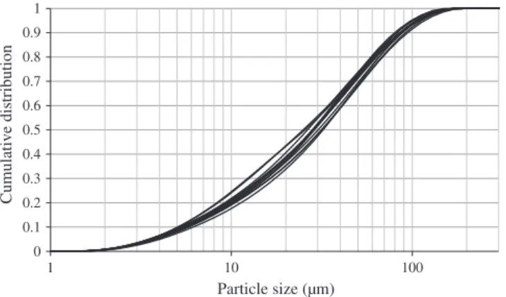
Feed size distributions were measured with a Malvern Mastersizer 2000HydroS.Fig. 1shows the cumulative feed size distributions for the 13
measurements.
The mean values of the mass fractions "f&iand covariance matrix cov(fi°,fj°) were calculated for every one of the n particle size classes from the
13 feed size distributions measured with the laser size analyser (Fig. 1). The superscript ‘°’ is used to denote that it is a reference particle size
distribution that will be used later for analysis of individual data sets. The average values "f&iand corresponding 95% confidence intervals are
plot-ted inFig. 2, under Student's t-distribution assumption with 13-1 = 12 degrees of freedom.
With the experiments used here, it is believed that our measurement conditions meet the requirements for a precise measurement of particle
size distribution by laser particle sizing as discussed by Xu and Di Guida[14]. Firstly, feed sampling and sub-sampling protocol is the same for all
13 samples, so that it can be assumed that the masses of solid and water used for the laser size analyses are invariant. The feed particles are fine
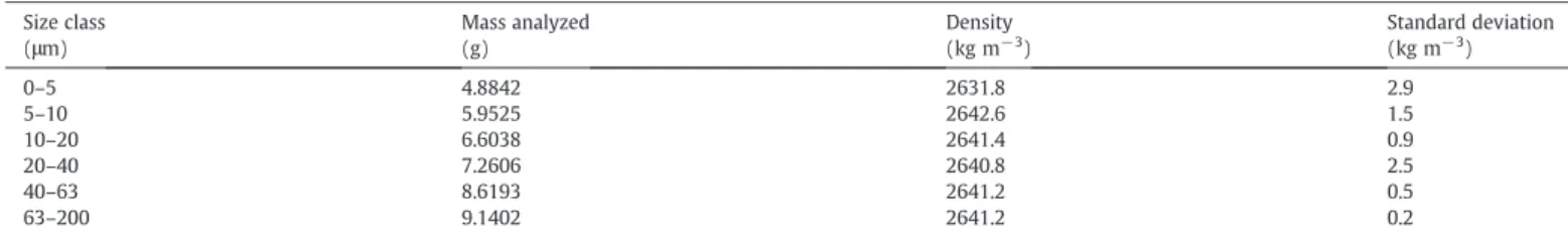
(minus 200 μm) ground quartz particles (SIBELCO Millisil® C6) that assay over 98.8% SiO2. To eliminate the possibility that measured partition
function variations may be affected by size-density variations, particle density was measured experimentally by Helium pycnometry as a func-tion of particle size. A 100 g feed sample was first microsieved into 6 size fracfunc-tions: 0 × 5 μm, 5 μm×10 μm, 10 μm×20 μm, 20 μm×40 μm,
40 μm × 63 μm and 63 × 200 μm. Measured density and corresponding standard deviation for each feed size fraction are given inTable 1. The
data confirm the invariance of particle density in the experiments. In addition,Fig. 3shows an SEM photomicrograph of the silica particles
used in the hydrocyclone tests, which confirms that particle shape is relatively uniform across the particle size range.
Looking at the relative standard deviation (RSD) for the fi°, which is plotted inFig. 4as a function of particle size, it appears that the RSD values
are relatively uniformly distributed, with the exception of few extreme RSD values that occur on both ends, when the measured mass fractions
are insignificant, of the order of 10−8or so. We can conclude that measurement error for individual mass fractions can be approximated by an
average RSD value. Here, an average value of RSD of 8.4% gives a good description of the experimental RSD.
0 0.1 0.2 0.3 0.4 0.5 0.6 0.7 0.8 0.9 1 1 10 100 Cumulative distribution Particle size (µm)
Fig. 5zooms on the data fromFig. 4in the domain that does not include the highest RSD values. Even though the average value of RSD is 8.4%, which may give a good description of the experimental RSD, there is still a noticeable variation of RSD as a function of particle size, which we
note RSD(fi°). Moreover, this variation appears quite marked in the 10 μm region where the fish-hook effect is known to occur.
To assess the level of quality of our data, we reviewed comparable data obtained by Xu and Di Guida[14]on laser diffractometry of glass
spheres. The RSD values obtained by the authors, as shown inTable 2, lie in the range of those obtained in this work.
The match between their RSD values and ours indicates that the laser sizing measurement errors controlled the error in our measurements, which is an indirect confirmation of the quality of the sampling and handling steps used to sample the hydrocyclone feed.
The last issue that should be discussed is that of the calculation of the covariance matrix VXfor the feed, underflow and overflow size
distri-butions for one particular experiment, for which fi, uiand oihave been measured. Analysis of the 13 size distributions through Pearson product–
moment correlation showed some degree of correlation between the measured mass fractions. These correlations were deemed low enough however to assume that the measured mass fractions are only weakly correlated. This justifies the setting of the covariance terms to zero as perSection 2.2.
The standard deviations of the n size fractions of the 3 streams are scaled directly from the size-dependent relative standard deviation (RSD)
of the reference feed size distribution f° using Eq.(8).
s fð Þi " fi ¼ s uð Þi " ui ¼s oð Þi " oi ≡s f & i ) * " fi& for i;j ¼ 1;n ð8Þ
Although it is possible to scale the covariance terms in the same manner, it is recalled here that covariance terms in VXare set equal to zero.
2.3. Illustrative example of partition function estimation
The mass balance calculations that follow are done in 2 ways, in order to strengthen the analysis and assess its sensitivity to the proper accounting for the errors associated with the particle size distribution measurements:
• The first set of calculations uses the average RSD of 8.4% calculated earlier, which is applied to all the mass fractions in all 3 stream size
distributions irrespective of particle size.
• The second set of calculations uses the size dependent RSD as per Eq.(8)and the size-dependent values RSD f2 i&
3 ¼s f
& i
ð Þ
f&
i data fromFig. 4instead.
-0.01 0 0.01 0.02 0.03 0.04 0.05 0.06 0.07 1 10 100 Frequency distribution Particle size (µm)
Fig. 2. Distribution of mass fractions fi°with their 95% confidence interval estimated from analysis of 13 hydrocyclone feed size distribution samples.
The mass balance calculations were performed with the 2 methods above using a data set obtained with a 100 mm diameter HC100 hydrocyclone from Neyrtec that was fitted with an 18 mm diameter spigot and 33 mm diameter vortex finder. It was operated at a feed mass
flow rate of 2.6 × 10⁻³m3s−1and an operating pressure of 105Pa. The feed to the hydrocyclone was characterized in the previous section.
This illustrative example corresponds to a test with a feed solids concentration of 20 wt.%.
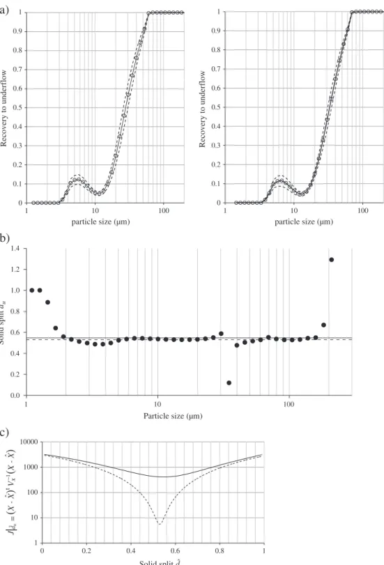
Key results from the mass balance calculations are given inFig. 6.
Fig. 6a and b show that differences in the mass balance outputs are marginal only between the two calculations, although mass balancing is
clearly more effective with the size dependent RSD(fi°) than with the average RSD(fi°) value of 8.4%. This is best seen inFig. 6c, which shows a very
clear minimum of the objective function with the second method. It is worth noting that both approaches yield slightly different estimates of the solids split to underflow in this example, namely 54.72% with the average value of RSD against 52.96% with the size-dependent RSD.
There is no significant difference in prediction of the recovery curve to underflow with the 2 approaches, as seen inFig. 6a; however careful
analysis shows a slightly narrower confidence interval with the 2nd method, confirming that it clearly is the best approach from a mass balancing perspective. Nevertheless, for all practical purposes, these calculations establish that mass balancing around a hydrocyclone can be done reliably with the average RSD value.
This section has also shown that it is a simple enough matter to estimate the confidence interval of the partition function of a hydrocyclone; hence there is no justification for not estimating it in practice or not reporting it in written work. More importantly, estimation of the error around the partition function is invaluable information for analyzing the performance of a hydrocyclone. It is this very information that is
used inSection 3below to investigate the fish-hook effect.
3. Proof of the “existence” of the fish-hook effect
The purpose of the previous section was to present and validate the mass balance calculation that yields estimation of the partition function and associated confidence interval, taking into account the particle size distribution measurement errors. For the sake of
trans-parency, it is recalled that the same distribution RSD(fi°) was applied
to all 3 streams as per Eq.(8), excluding the possibility that sampling
and preparation errors may be different between the 3 streams. This is an assumption that could only be lifted by sampling all 3 streams several times, which was not done here. However, given that the tests were performed in a controlled laboratory environment with recirculation of the underflow and overflow streams to a feed sump, it is not expected that sampling errors would differ significantly between the streams.
In the case of the illustrative example ofSection 2.3., a fish-hook
effect was observed (seeFig. 6a). The narrowness of the confidence
interval of the partition function around the dip and critical points,
as defined by[6], excludes the possibility of size distribution
measure-ment errors being the source of the fish-hook effect in this particular experiment.
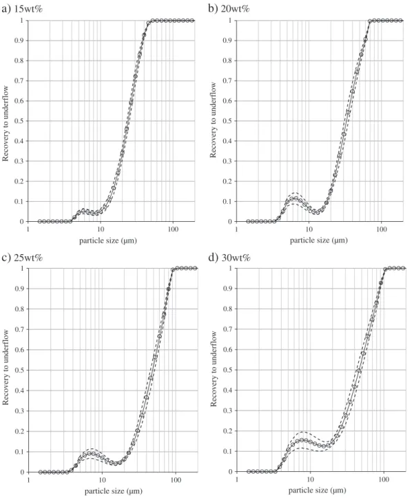
Partition functions were calculated using the mass balancing pro-cedure presented above for a test series that covered dilute to dense regime with the same hydrocyclone and feed size distribution as perSection 2. With the hydrocyclone set-up and operating conditions reported previously, feed solids concentration was varied from 15 wt.% to 50 wt.% in 5 wt.% increments. Raw measurements of particle size
dis-tributions can be found in Appendix A of Davailles' PhD dissertation[11].
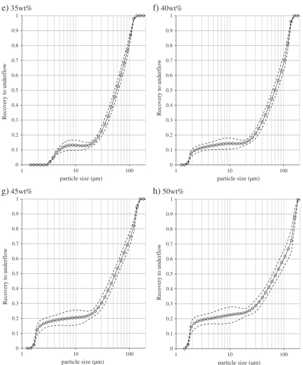
The estimated partition functions are plotted inFig. 7a to h. Feed
solids concentration is reported below each figure.
Below a feed solids concentration of 10 wt.% and above 40 wt.%, the partition function does not appear to exhibit the fish-hook effect for this particular hydrocyclone setting and operating conditions. Between 15 wt.% and 35 wt.%, the fish-hook effect is clearly visible.
Table 1
Validation of the invariance of particle density with particle size by He-pycnometry. Size class (μm) Mass analyzed (g) Density (kg m−3) Standard deviation (kg m−3) 0–5 4.8842 2631.8 2.9 5–10 5.9525 2642.6 1.5 10–20 6.6038 2641.4 0.9 20–40 7.2606 2640.8 2.5 40–63 8.6193 2641.2 0.5 63–200 9.1402 2641.2 0.2 0% 20% 40% 60% 80% 100% 120% 140% 160% 1 10 100 RSD (%) Particle size (µm)
Fig. 4. RSD (%) values for particle size distribution assays fi°in all the measured size
classes. 0% 2% 4% 6% 8% 10% 12% 14% 16% 1 10 100 RSD (%) Particle size (µm)
To further confirm the significance of the fish-hook effect, the values and 95% confidence interval of the dip and critical points are plotted inFig. 8as a function of feed solids concentration.
Within the range of solids concentration where the fish-hook was
visually observed,Table 3gives the levels of significance of the
fish-hook effect as a function of feed solids concentration, which we define as the level of significance of the difference between the estimated dip and critical point values.
With the 20 wt.% and 25 wt.% feed solids concentration tests, the fish-hook effect is the most significant at the confidence level of 99.8% and higher. At 15 wt.% and 30 wt.%, the significance of the fish-hook effect is 66% and 62% respectively. At 35 wt.%, its significance
is less than 3%, and above 35 wt.% it was not detected (SeeFig. 7f,
g and h).
Table 2
Data calculated from laser diffraction measurements published by Xu and Di Guida (2003,Table 1p. 147 and Table 2 p. 148).
Monomodal glass spheres Bimodal glass spheres ^ d ¼ 65:27μm d^1¼ 46:47μm d^2¼ 96:43μm RSD = 7.7% RSD = 13.6% RSD = 8.4% 0 0.1 0.2 0.3 0.4 0.5 0.6 0.7 0.8 0.9 1 1 10 100 Recovery to underflow particle size (µm) 0 0.1 0.2 0.3 0.4 0.5 0.6 0.7 0.8 0.9 1 1 10 100 Recovery to underflow particle size (µm) 0.0 0.2 0.4 0.6 0.8 1.0 1.2 1.4 1 10 100 Solid split du Particle size (µm)
a)
b)
1 10 100 1000 10000 0 0.2 0.4 0.6 0.8 1 Solid split duc)
ˆWe have shown in this section that, under some operating condi-tions, the fish-hook effect can occur at a significance level that excludes the possibility of measurement errors being a probable cause. In other words, the fish-hook effect is a real phenomenon whose origin goes back to the physics of particle transport inside the hydrocyclone.
4. Discussion
4.1. Origin of the fish-hook
The conditions that will yield the fish-hook phenomenon to be significant can be numerous, and it should not be inferred from the data that were presented in the previous section that the fish-hook is most significant in the 20–30 wt.% region only. Indeed, many con-figurations and operating conditions can lead to the fish-hook effect. Further discussion on this is outside the scope of this article.
4.2. Appearance of randomness and sporadicity of the fish-hook effect By refuting the possibility that measurement errors could be the rea-son beyond the fish-hook effect, we have now established beyond doubt that the fish-hook effect is not a random effect. What could then possibly explain that a number of researchers, like Nagaswarareo
[8]claim it is random and sporadic? One possible way of answering
this is to ask ourselves whether it could be possible for the fish-hook effect to be present and for the observer not to observe it, giving an impression of randomness and sporadicity.
In this paper, we have demonstrated the significance of the fish-hook effect based on analysis of the error of the estimate of the recov-ery curve. It is often the case that recovrecov-ery curves are calculated
with-out any indication of their confidence bounds.Fig. 9illustrates the
idea that it is possible, in principle, to obtain a high degree of variabil-ity in fish-hook measurement if one does not account for the confi-dence bounds of the partition function. Starting with the earlier
0 0.1 0.2 0.3 0.4 0.5 0.6 0.7 0.8 0.9 1 1 10 100 Recovery to underflow particle size (µm)
a)
15wt%
0 0.1 0.2 0.3 0.4 0.5 0.6 0.7 0.8 0.9 1 1 10 100 Recovery to underflow particle size (µm)b)
20wt%
0 0.1 0.2 0.3 0.4 0.5 0.6 0.7 0.8 0.9 1 1 10 100 Recovery to underflow particle size (µm)c)
25wt%
0 0.1 0.2 0.3 0.4 0.5 0.6 0.7 0.8 0.9 1 1 10 100 Recovery to underflow particle size (µm)d)
30wt%
partition function whose fish-hook effect is significant at more than
60% level,Fig. 9shows that it is possible to draw a partition function
that shows a sharp fish-hook or no fish-hook inside the bounds of the
95% confidence interval of the partition function. It is this error asso-ciated with measurement of the partition function which the authors believe can in part explain the appearance of randomness and sporadicity of the fish-hook effect that has been reported by some authors.
This possible explanation for the apparent randomness and sporadicity appears even more when considering that these effects could be obtained with a partition function that is measured in the laboratory, under well controlled operating conditions. If we now
0 0.1 0.2 0.3 0.4 0.5 0.6 0.7 0.8 0.9 1 1 10 100 Recovery to underflow particle size (µm)
e)
35wt%
0 0.1 0.2 0.3 0.4 0.5 0.6 0.7 0.8 0.9 1 1 10 100 Recovery to underflow particle size (µm)f)
40wt%
0 0.1 0.2 0.3 0.4 0.5 0.6 0.7 0.8 0.9 1 1 10 100 Recovery to underflow particle size (µm)g)
45wt%
0 0.1 0.2 0.3 0.4 0.5 0.6 0.7 0.8 0.9 1 1 10 100 Recovery to underflow particle size (µm)h)
50wt%
Fig. 7 (continued). 0.00 0.05 0.10 0.15 0.20 0.25 0.30 10% 15% 20% 25% 30% 35% 40% 45% 50% Recovery to underflowFeed solids concentration (wt%)
dip point (Pd) Critical point (Pc)
no fish-hook fish-hook region
Fig. 8. Comparison between dip point and critical point measurements.
Table 3
Significance of the fish-hook effect as a function of solids concentration in the conditions of the experiment.
Feed solids concentration 15 wt.% 20 wt.% 25 wt.% 30 wt.% 35 wt.% Significance level 66.23% 99.99% 99.80% 62.30% 2.85%
consider the same measurements in the plant, where operating con-ditions may fluctuate, the possibility of missing the fish-hook effect for a particular measurement can be greater.
5. Conclusions
Based on the aforementioned results and discussion the following conclusions may be drawn:
• Estimation of confidence bounds of the partition function is of
significant value for analysis of the performance of a hydrocyclone.
• Partition functions estimated from carefully generated experimental
data set in a 100 mm diameter hydrocyclone followed by rigorous statistical analyses of the data have completely ruled out the possibil-ity of measurement errors as the cause of the observed fish-hook effect. This conclusion implies that the fish-hook phenomenon is of physical origin.
•Statistical arguments have also been put forward to explain why in
some situations the fish-hook effect may appear to be random and sporadic.
Notations Symbols
du Solid mass flow split to the underflow
f Vector of mass fractions in the feed stream
u Vector of mass fractions in the underflow stream
o Vector of mass fractions in the overflow stream
n Number of particle size classes
Subscripts
i,j Indices of particle size class
Superscripts
^ Circumflex symbol denotes the estimate of a random variable
t Transpose of a vector or matrix
References
[1] R. Del Villar, J.A. Finch, Modelling the cyclone performance with a size dependent entrainment factor, Minerals Engineering 5 (6) (1992) 661–669.
[2] J.A. Finch, Modelling a fish-hook in hydrocyclone selectivity curves, Powder Technology 36 (1983) 127–129.
[3] B.C. Flintoff, L.R. Plitt, A.A. Turak, Cyclone modeling – a review of present technology, CIM Bulletin 69 (1987) 114–123.
[4] W. Kraipech, W. Chen, F.J. Parma, T. Dyakowski, Modelling the fish-hook effect of the flow within hydrocyclones, International Journal of Mineral Processing 66 (2002) 49–65.
[5] A.K. Majumder, P. Yerriswamy, J.P. Barnwal, The “fish hook” phenomenon in centrifugal separation of fine particles, Minerals Engineering 16 (2003) 1005–1007. [6] A.K. Majumder, H. Shah, P. Shukla, J.P. Barnwal, Effect of operating variable on shape of “fish-hook” curves in hydrocyclones, Minerals Engineering 20 (2007) 204–206.
[7] B. Wang, A.B. Yu, Computational investigation of the mechanisms of particle separation and “fish-hook” phenomenon in hydrocyclones, AICHE Journal 56 (7) (2010) 1703–1715.
[8] K. Nageswararao, A critical analysis of the fish hook effect in hydrocyclone classifiers, Chemical Engineering Journal 80 (2000) 251–256.
[9] S.K. Kawatra, T.C. Eisele, Causes and significance of inflections in hydrocyclone efficiency curves, in: Advances in Comminution, The Society for Mining, Metallurgy and Exploration, Littleton, CO, 2006, pp. 131–147.
[10] C. Bazin, D. Hodouin, Importance of covariance in mass balancing of particle size distribution data, Minerals Engineering 14 (8) (2001) 851–860.
[11] Davailles, A., 2011. Effet de la concentration en solide sur les performances de separation d'un hydrocyclone (simulations numériques et experiences de references), Ph.D. dissertation, The University of Toulouse, 197 pp.
[12] A. Davailles, E. Climent, F. Bourgeois, Fundamental understanding of swirling flow pattern in hydrocyclones, Separation and Purification Technology 92 (2011) 152–160.
[13] A. Davailles, E. Climent, F. Bourgeois, A.K. Majumder, Analysis of swirling flow in hydrocyclones operating under dense regime, Minerals Engineering 31 (2012) 32–41.
[14] R. Xu, A.A. Di Guida, Comparison of sizing small particles using different technologies, Powder Technology 132 (2003) 145–153. 0 0.1 0.2 0.3 0.4 0.5 0.6 0.7 0.8 0.9 1 1 10 100 Recovery to underflow particle size (µm)


![Varicella. To be [vaccinated] or not to be: that is the question!](data:image/gif;base64,R0lGODlhAQABAIAAAP///wAAACH5BAEAAAAALAAAAAABAAEAAAICRAEAOw==)