Atmospheric correction and inherent optical property estimation in the southwest New Caledonia lagoon using AVNIR-2 high-resolution data

HAL Id: ird-00862977

https://hal.ird.fr/ird-00862977

Submitted on 18 Sep 2013

HAL is a multi-disciplinary open access

archive for the deposit and dissemination of sci-entific research documents, whether they are pub-lished or not. The documents may come from teaching and research institutions in France or abroad, or from public or private research centers.

L’archive ouverte pluridisciplinaire HAL, est destinée au dépôt et à la diffusion de documents scientifiques de niveau recherche, publiés ou non, émanant des établissements d’enseignement et de recherche français ou étrangers, des laboratoires publics ou privés.

Atmospheric correction and inherent optical property

estimation in the southwest New Caledonia lagoon using

AVNIR-2 high-resolution data

Hiroshi Murakami, Cecile Dupouy

To cite this version:

Hiroshi Murakami, Cecile Dupouy. Atmospheric correction and inherent optical property estimation in the southwest New Caledonia lagoon using AVNIR-2 high-resolution data. Applied optics, Optical Society of America, 2013, 52 (2), pp.182-198. �ird-00862977�

1

Atmospheric correction and inherent optical property

estimation in the southwest New Caledonia lagoon using

AVNIR-2 high-resolution data

4

Hiroshi Murakami1,*, Cécile Dupouy2

5

1

Japan Aerospace Exploration Agency, Earth Observation Research Center, 2-1-1, Sengen, 6

Tsukuba, Ibaraki, Japan 305-8505 7

2

Aix-Marseille University, University of South Toulon Var, CNRS/INSU, IRD, MIO, UM 110 8

Centre IRD of Noumea, BP A5, 98848, Noumea, New Caledonia 9

*Corresponding author: murakami.hiroshi.eo@jaxa.jp 10

Abstract

11

Retrievals of inherent optical properties (IOPs) and Chlorophyll-a concentration (Chla) was 12

investigated for AVNIR-2 images with 30-m spatial resolution and four bands in the southwest 13

tropical lagoon of New Caledonia. We corrected the atmospheric and sea-surface reflectance 14

iteratively through the retrieval of IOPs. After an additional correction of sea floor reflectance, 15

the estimated IOPs and Chla agreed well with the in situ measurements even in the lagoon 16

areas. This study provides a method to allowing a local optimal estimation of IOPs and Chla 17

with a high resolution sensor by preparation of the candidate spectra for the target areas. 18

2

1. INTRODUCTION

20

1.1 Ocean color retrievals in the coastal areas

21

Ocean color retrieval is a challenge in the coastal areas but is a powerful tool for coastal 22

surveys. Sea surface reflection, including sunglint and whitecap, cause significant errors in the 23

ocean color estimation [1,2,3]. Sea surface reflection can be estimated from a statistic scheme 24

such as that presented by Cox and Munk [4] using low-resolution wind speed data from a 25

microwave radiometer, a scatterometer, or objective analysis data (e.g., [5,6]). However, the 26

correction based on the wind speed data is problematic in coastal areas because of fine 27

variations in the distribution of surface reflection due to variable winds, fetch length, and air-28

sea stability caused by the fine structure of the coastal geography. Several studies have 29

investigated high spatial resolution sunglint correction using hyperspectral bands or small scale 30

glint variations (e.g. [7,8]). Murakami and Frouin [9] demonstrated the possibility of sunglint 31

(ρg) correction by using 500-m resolution near infrared (NIR) and shortwave infrared (SWIR)

32

bands of Moderate Resolution Imaging Spectroradiometer (MODIS). Higher (10-30 m) spatial 33

resolution sensors are expected to capture higher resolution spatial structures of ocean color 34

phenomena, especially in the coastal areas. However, they have a limited number of spectral 35

bands generally (e.g., without SWIR bands), which prevents the precise estimation of aerosol 36

properties and the distinction between aerosol and sea-surface reflection. 37

In addition to these sensor limitations, coastal areas present difficulties for ocean color 38

retrievals, i.e., high NIR reflectance by suspended matter, complex Inherent Optical Properties 39

(IOPs) due to various material inputs from the land, and bottom reflectance in the shallow areas. 40

This explains why the blue/green ratio of remote sensing reflectance (Rrs), which is

3 traditionally used in the empirical estimation of chlorophyll-a concentration (Chla), does not 42

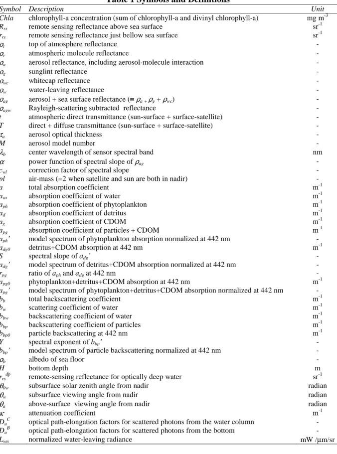
allow to calculate Chla in most cases of the coastal area (see Table 1 for symbol definitions 43

and units). 44

1.2 The New Caledonia lagoon

45

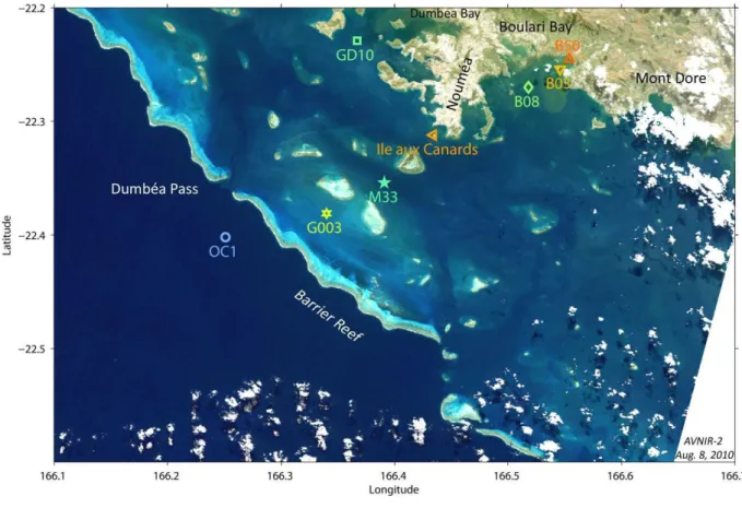
The New Caledonia lagoon is a large, almost continuous lagoon (22177 km2) lying in the 46

southwestern tropical Pacific from 20°S to 22°S and 166°E to 167°E (Fig. 1). Its heterogeneous 47

bathymetry (25 m as a mean depth) is due to a complex geomorphology with the presence of 48

sedimentary plains and a high proportion of shallow waters and numerous small sand islands 49

[10,11,12]. It is largely connected to the open ocean along its southern side, but only by narrow 50

passes in its southwestern side. It is an example of a coral reef lagoon system, which are very 51

sensitive to anthropogenic (nutrients, mining) perturbations [10,11] as well as to interannual 52

changes linked to the balance between dry El Niño and wet La Niña episodes [13,14], which 53

are amplified in lagoons [12]. The central lagoon is characterized by oligotrophic to 54

mesotrophic waters (yearly average chlorophyll-a concentration of 0.25 ± 0.01 mg m-3) [15,16] 55

and exhibits a strong seasonal cycle with higher values in austral winter (July) or austral 56

summer (February) during nitrogen-fixing Trichodesmium blooms [17,18,19,20]. Upwelling at 57

the barrier reefs [21] as well as internal waves in the southern part of the lagoon are two major 58

mechanisms of exchange with the sea, which can modify the phytoplanktonic assemblage [22]. 59

Rain can also induce large chlorophyll enrichments in the lagoon [23]. With relatively low 60

river inputs and a low turbidity range (0.20-16 g m-3), its trophic state is linked to spatial 61

variations in flushing times [12,16,24]. Similarly to “optically complex” Case 2 European 62

waters [25] or coastal bays [26], reflectance in the New Caledonia lagoon can be highly 63

4 variable [27] as in other tropical environments [28], the Australian Great Barrier Reef [29], 64

tropical estuaries [30] with a high influence of mineral particles from river discharge in bays 65

[31] or colored dissolved organic matter (CDOM) [32]. Additionally, bottom reflectance, 66

which represents a strong component in clear tropical shallow waters, may influence Rrs

67

[33,34,35,36]. 68

In order to improve the challenge of remote sensing in coastal environments [37], surface 69

water IOPs (absorption and backscattering) were measured during several observation 70

campaigns (e.g., coastal stations of Diapalis in 2003, Bissecote, Echolag, Valhybio, and the 71

Valhybio Monthly Survey cruises from 2006 to 2010) in the lagoon and at different seasons 72

[27,38,39]. The bathymetry of the Southern New Caledonia lagoon was compiled [12]. 73

1.3 ALOS AVNIR-2

74

Advanced Land Observation Satellite (ALOS) has been operated by JAXA from 24 Jan. 75

2006 to 12 May 2011 and carried the Advanced Visible and Near Infrared Radiometer type 2 76

(AVNIR-2). AVNIR-2 has four spectral bands (centered at 463 nm, 560 nm, 652 nm, and 821 77

nm) with a 10-m Instantaneous Field of View (IFOV), a 70-km Field of View (FOV) and a 78

mechanical pointing function (by moving mirror) along the cross-track direction (±44 deg) for 79

effective global land observation. To achieve the ALOS mission objectives (cartography, 80

regional observation, disaster monitoring, resources survey, and technology development) and 81

to expand to quantitative applications, such as determination of vegetation density, coastal 82

water color and their time dependencies, it is important to evaluate, improve and maintain the 83

radiometric calibration accuracy of AVNIR-2 (the pre-defined target is absolute error less than 84

10% [40]). The cross-calibration with MODIS indicated that the difference in top of 85

5 atmosphere (TOA) radiance is less than 3% in the visible bands, and the temporal stability of 86

the radiance is less than 2% per 1000 days [41]. 87

1.4 Scope of this study

88

Atmospheric and sea surface correction and IOP estimation were conducted using the four 89

bands of 30-m images averaged from AVNIR-2 10-m images (see section 2.1). The linear 90

matrix inversion (LMI) of IOPs [42,43,44] and atmospheric + surface reflection correction was 91

simplified to allow the four-band and high spatial resolution AVNIR-2 retrievals. Influence of 92

the bottom reflectance was reduced by using bathymetry data with a unique spectrum of 93

bottom reflectance. We compared the IOP estimates by different candidate IOP spectra 94

(observed particles + CDOM absorption (apg) and particle backscattering (bbp) spectra) in the

95

LMI scheme. Chla was estimated by two ways, from a statistical relationship with apg, or from

96

blue/green ratio of Rrs. For the series of AVNIR2 images available over the New Caledonia

97

lagoon, we validated the derived IOPs (apg and bbp) and Chla using in situ measurements

98

around the AVNIR-2 observation dates. 99

2. DATA AND METHODS

100

2.1 AVNIR-2 images and radiance correction

101

AVNIR-2 data have 10-m spatial resolution but only 8-bit digital resolution with relatively 102

low gain designed for the land-surface observations. We averaged AVNIR-2 TOA radiance 103

images to a 30-m (0.0003 degrees equal latitude-longitude) grid to reduce the sensor noise 104

before the atmospheric correction because the ocean-color signal is much lower than 105

atmospheric one in the visible wavelengths. 106

6 The AVNIR-2 in-orbit radiometric performance was evaluated through a comparison with 107

Aqua MODIS by the cross-calibration scheme[41]. This scheme uses the TOA reflectance 108

functions of the satellite zenith angle estimated by Aqua MODIS observations within ±16 days 109

from the AVNIR-2 observation over temporally and spatially stable ground areas. The cross 110

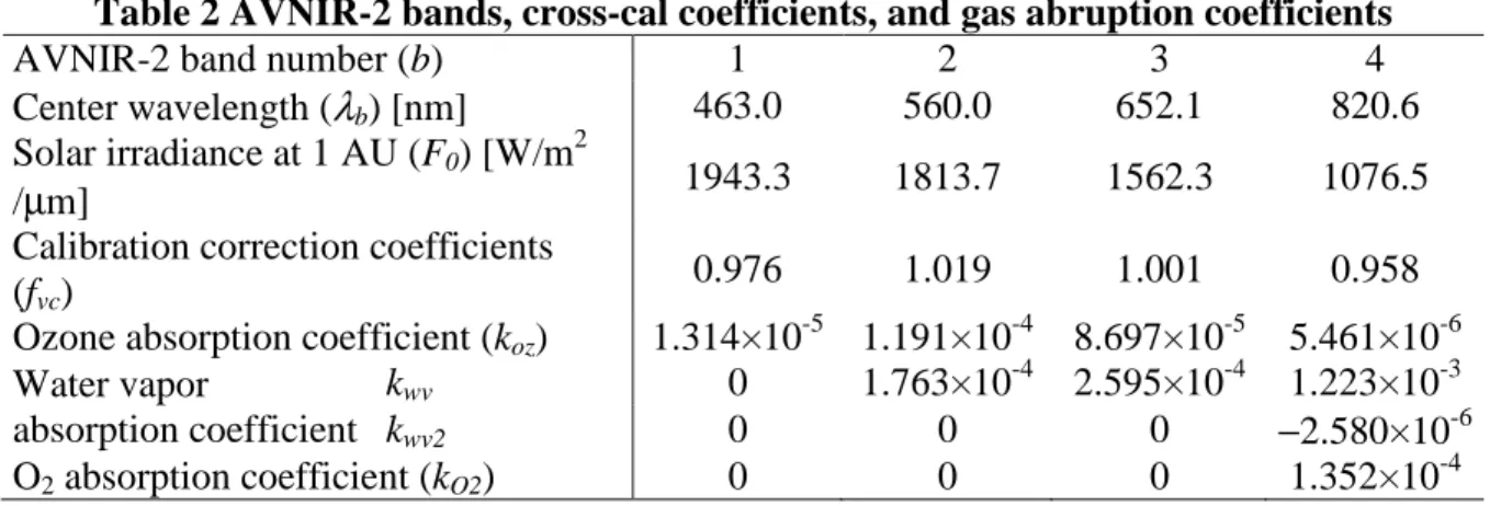
calibration with the Aqua MODIS over the Antarctic snow fields allow us to correct AVNIR-2 111

bands 1-4 by the correction coefficients shown in Table 2. We calculated the TOA reflectance 112

of standard gas absorption conditions (column ozone = 343.8DU, water vapor = 14.19 mm, and 113

pressure = 1013.25 hPa) from the AVNIR-2 radiance observation as shown in Appendix. 114

Seventeen clear AVNIR-2 scenes were captured around the target area in the ALOS 115

mission period. The dates were 10 Sep. and 27 Sep. in 2006, 12 Feb., 3 Mar., 15 May, and 31 116

Jul. in 2007, 31 Oct. and 17 Nov. in 2008, 3 Sep. and 20 Nov. in 2009, 5 Jan., 3 Feb., 21 Mar., 117

8 Aug., and 22 Dec. in 2010, and 24 Mar. and 10 Apr. in 2011. Some scenes (27 Sep. 2006, 12 118

Feb. 2007, 31 Oct. and 17 Nov. 2008, 20 Nov. 2009, and 5 Jan. 2010) were covered by the 119

sunglint. Match-ups with in situ measurements were obtained (total 15 points) on 3 Sep. 2009 120

(time difference from the AVNIR-2 observation ∆D=5 days), 17-18 Nov. 2009 (∆D=2 days), 121

and 11 Jan. 2010 (∆D=6 days). 122

2.2 Simplification of the atmospheric and surface corrections

123

At each solar and sensor geometry condition, the TOA reflectance ρt,, for which gaseous

124

absorption is normalized by standard atmosphere condition, can be described as follows. 125

ρt(λb) = ρr(λb) + ρa(λb, τa, M) + t(λb, τa, M)× ρg(λb) + T(λb, τa, M)× ρwc(λb) + T(λb, τa, M)

126

×ρw(λb) (1)

7 where ρr is the atmospheric molecule reflectance, ρa is the aerosol reflectance, including

128

aerosol-molecule interaction, ρw is the water-leaving reflectance, ρg is the sunglint reflectance,

129

ρwc is the whitecap reflectance, t is the atmospheric direct transmittance (sun-surface +

surface-130

satellite), and T is the direct + diffuse transmittance (sun-surface + surface-satellite), λb is the

131

center wavelength of sensor spectral band, τa is the aerosol optical thickness, and M is the

132

aerosol model. ρg can be estimated by a statistical equation [4] using wind speed and the

133

refractive index of water at each wavelength. However, there is no simultaneous 30-m 134

resolution wind speed data, and the statistical relation is not always consistent with the real 135

complicated sea surface. 136

The Rayleigh scattering of ρr and T (at τa=0) can be estimated by atmospheric radiative

137

transfer simulation. In order to achieve this, we used Pstar2b [45], which takes into account 138

atmospheric polarization, provided by the National Institute for Environmental Studies (NIES) 139

GOSAT project and the OpenCLASTR project [46,47,48]. We prepared look-up tables of 140

ρr(λb) (including sea-surface reflection with wind speed = 0) and T at each geometric condition.

141

The Rayleigh-scattering subtracted reflectance (ρagw) can be described by the following Eq.

142 (2). 143 ρagw(λb) ≡ (ρt(λb) −ρr(λb)) / T(λb, τa=0) 144 = [ ρa(λb, τa, M) / T(λb, τa=0) + t(λb, τa, M) / T(λb, τa=0)× ρg(λb) + T(λb, τa, M) / T(λb, 145 τa=0) ×ρwc(λb) ] + T(λb, τa, M) / T(λb, τa=0) ×ρw(λb) (2) 146

The T(λb=1,2,3 and 4, τa=0) are about 0.83, 0.91, 0.95, and 0.98 respectively at θsun=θsat=0. T(λb, τa,

147

M) / T(λb,τa=0) can be approximated as 1.0 because it is >0.9 when τa<0.5. We simplified

148

aerosol and surface reflection (ρag ≡ρa +ρg ) as the following form (Eq. (3)) because ρag is to

8 be spectrally smooth and can be approximated by a power function α of the wavelength ratio in 150

most cases [49]. 151

ρag(λb) ≅ρag(821 nm) × (λb× cwl / 821 nm)α (3)

152

The spectral shape of ρag was improved by a correction factor, cwl (= 0.99 at band 3 (652 nm)

153

and 1.0 at other bands), which was derived from the atmospheric radiative transfer simulation 154

(the root mean square error of ρag is 0.004 at 463 nm for the tropospheric, oceanic, and their

155

mixed aerosols in the case of aerosol optical thickness = 0.3 and air-mass pl < 4). The α ranged 156

from −0.5 to +0.3 for the oceanic aerosols and from −1.8 to −1.2 for the tropospheric aerosols. 157

The variables about the aerosol and surface reflection, α and ρag (821 nm), could be

158

estimated using the AVNIR-2 data through an iteration with the IOP retrieval described in the 159

next section. The approximation of Eq. (3) enabled quick processing including the iteration 160

scheme. 161

2.3 IOP and water-leaving reflectance estimation

162

Most of the IOP algorithms [50] are based on the equation of remote sensing reflectance 163

below the surface (rrs), the total absorption coefficient (a) and the backscattering coefficient

164

(bb) proposed by Gordon et al. [51].

165 rrs(λ) = g1× u(λ) + g2× u(λ)2 (4) 166 a(λ) = aw(λ) + aph(λ) + ad(λ) + ag(λ) (5) 167 bb(λ) = bbw(λ) + bbp(λ) (6) 168 with 169 u(λ) = bb(λ) / ( bb(λ) + a(λ) ) (7) 170

9 where g1=0.0949 and g2=0.0794 [51]. aw, aph, ad, and ag are the absorption spectra of water,

171

phytoplankton, detritus, and CDOM respectively. bbw and bbp are backscattering coefficients of

172

water and particles. Remote sensing reflectance above the surface, Rrs is estimated from rrs

173

using the relation from [51,52] as: 174

Rrs(λ) = 0.52 × rrs(λ) / (1− 1.7× rrs(λ)). (8)

175

The water-leaving reflectance ρw in (1) is simply calculated from the Rrs.

176

ρw(λ) = π× Rrs(λ) (9)

177

We used the LMI scheme [42,43,44] to estimate IOPs. The scheme requires aw, bbw, and

178

model spectra, aph’, adg’ (absorption of detritus + CDOM), and bbp’, which is normalized at a

179

specific wavelength (442 nm was used in this study). We used aw and bbw values from [53,54]

180

weighted by the AVNIR-2 spectral response (shown in Table 3). Wavelength functions of adg

181

and bbp were as follows.

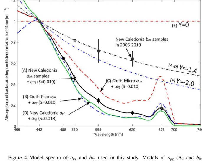
182 adg(λb) = adg0× adg(λ)’ (10) 183 bbp(λb) = bbp0× bbp(λb)’ (11) 184 where 185 adg(λ)’ = exp(S × (λ− 442)) (12) 186 bbp(λ)’= (λ /442)Y (13) 187 where adg0 is adg at 442 nm, bbp0 is bbp at 442 nm, S= −0.010 or −0.018, and Y= −1.4, 0, or +2. S 188

= −0.010 and Y = −1.4 were derived from the New Caledonia in situ measurements of adg and

189

bbp respectively.

10 The inversion process was simplified to use only two IOP parameters, apg (≡ ap+ag ≡

191

aph+adg) and bbp, and two AVNIR-2 bands, band 1 (463 nm) and band 2 (560 nm). We set the

192

apg’ as follows.

193

apg(λb) = apg0× apg(λb)’ = apg0× { (1− rpg)× aph(λb)’ + rpg× adg(λb)’ } (14)

194

where apg0 is apg at 442 nm. The ratio of aph and adg at 442 nm, rpg, was set to 0.52 / (1 + 0.52)

195

considering the normal conditions observed in the New Caledonia in situ data [32]. We can 196

estimate two parameters of IOPs, apg0 and bbp0, by the iteration processes of the IOP forward

197

calculation and LMI [42,43,44]. 198

If we have an initial value of apg0 and bbp0, ρw can be calculated by (4)-(14). Using the ρw,

199

ρag at 652 nm and 821 nm can be calculated using molecular scattering corrected reflectance

200

derived from satellite observation (ρagw) as:

201

ρag(λ) = ρagw(λ) −ρw(λ) (15)

202

where λ = 652 nm and 821 nm. Considering an approximation of Eq. (3), α can be calculated 203

by Eq. (16). 204

α = log( ρag(652 nm) / ρag(821 nm) ) / log(652×cwl / 821) (16)

205

Then, ρw at 463 nm and 560 nm are calculated by Eqs. (3) and (15). Using the ρw at the two

206

visible bands, apg0 and bbp0 can be calculated by the LMI [42,43,44].

207

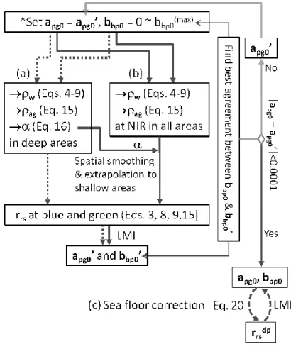
The iteration process to derive the final value of apg0 and bbp0 is shown in Fig. 2. The first

208

process aims to estimate α except for shallow areas (bathymetry<20m) where the bottom 209

reflectance can influence rrs. The iteration was repeated to find optimal values of apg0 and bbp0

11 by minimizing the difference between bbp0 preset in Eq. (11) and bbp0 calculated by the

211

inversion matrix. The initial value of apg0’ was set to 0.01, which does not affect the final apg0

212

estimates because apg is relatively small in the total a in red and NIR wavelengths. The

sub-213

process is repeated until | apg0− apg0’ |<0.0001 (practically less than four times in most pixels)

214

with revision of apg0 and the search range of bbp0 (bbp0(max)) which is set by ρag at 821 nm and

215

the extremely high apg0 = 20 m-1. After completing the first process, we smoothed α for each

216

0.1 deg × 0.1 deg area to reduce the AVNIR-2 sensor noise and extrapolate to the shallow 217

(<20m) areas where we did not estimate α in the first process. The second process derives ρag

218

apg, bbp, and Rrs for every 30-m grid using the same equations. We can derive IOPs and Rrs at

219

any wavelengths (AVNIR-2 bands at 463 nm and 560 nm and the wavelengths of the in situ 220

measurements at 442 nm and 555 nm) using the IOP spectra apg(λ)’ and bbp(λ)’ (see section

221

2.5). 222

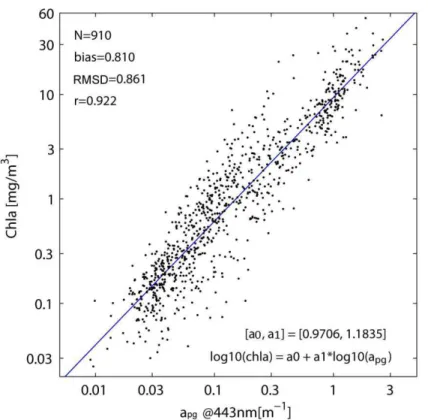
2.4 Chlorophyll-a estimation

223

Chlorophyll-a was estimated by regression of apg(442 nm) and the empirical blue/green as

224

follows: 225

log10(Chla) = 0.9706 + 1.1835 × log10(apg(442 nm)) (17)

226 log10(Chla) = 0.1464 − 1.7953 r + 0.9718 r2− 0.8319 r3− 0.8073 r4 (18) 227 where 228 r = log10( Rrs(463 nm) / Rrs(560 nm) ). (19) 229

The relationship between Chla and apg(443 nm) was derived from apg and the fluorometric

230

chlorophyll-a data included in the bio-Optical Marine Algorithm Data set (NOMAD) [55] (Fig. 231

3). The MODIS OC2M-HI equation developed by the NASA Ocean Biology Processing Group 232

12 (OBPG) using the NOMAD database [6] was used for the two channel equation because 233

AVNIR-2 has only two channels in blue and green wavelengths. 234

2.5 In situ bio-optical measurements

235

Field measurements of the two IOPs, the absorption coefficient, a, and the backscattering 236

coefficient, bb, were obtained at stations in the southwest part of the lagoon (Fig. 1) during

237

various seasons from 2006 to 2010. The bb was measured with a Hydroscat-6 profiler (H6:

238

HobiLabs, wavebands (λ) centered at 442, 488, 510, 550, 620 and 670 nm with a bandwidth of 239

10 nm for the 442–550 nm bands and 20 nm for the 620 and 670 nm bands) [19,27]. The 240

particulate back-scattering coefficient, bbp(λ), was calculated by subtracting from bb(λ) the

241

theoretical “pure water spectrum”, bbw(λ) (calculated as bbw(λ) = 0.5× bw(λ)) [51]. The

242

particulate absorption coefficient, ap(λ), was measured with the filter-pad technique [56] using

243

water samples filtered onto 25-mm GF/F Whatman filters. For pigments, the filters were 244

dipped in 5.4 ml 100% acetone (final concentration 90% acetone taking into account water 245

retention by the filter, e.g., 0.621 ± 0.034 ml) and ground with the freshly broken end of a glass 246

rod for chlorophyll and phaeopigment extraction [57]. For comparison with the satellite-247

estimated Chla, we used the sum of chlorophyll a and divinyl chlorophyll a, Chla (in mg m-3), 248

as measured by spectrofluorometry, and well correlated with fluorometry in the Caledonian 249

lagoon [15,27]. 250

For the LMI, we prepared the model spectra of apg and bbp optimized for the New

251

Caledonia in situ samples (six samples of aph and adg in 2003, and 112 samples of bbp in

2006-252

2010). The samples of aph and adg were distributed around the lagoon of the southeast New

253

Caledonia, but not near bays of the mainland. The spectral shape adg’ and bbp’ (relative values

13 from λ=442 nm) were modeled by Eqs. (12) and (13) respectively. The model spectra from the 255

averages of the New Caledonia measurements were used as the standard in sensitivity tests 256

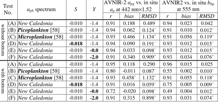
described below. 257

We tested the sensitivity of different sets of model spectra: (A) apg’ and bbp’ from the New

258

Caledonia measurements (e.g., same as the above); (B) same as (A) but aph’ from a

259

picoplankton spectra [58]; (c) same as (A) except for aph’ from a microplankton spectra [58];

260

(D) same as (A) except for adg’ with S = −0.018; (E) same as (A) except for bbp’ with Y = 0.0;

261

and (F) same as (A) except for bbp’ with Y = −2.0 (Fig. 4). These aph’ spectra are listed in Table

262 3. 263

2.6 Correction of sea floor reflection

264

The Rrs and IOP estimation might be influenced by bottom reflectance especially in low

265

absorption and shallow areas, such as site G003 near the barrier reef (11 meters depth, bottom 266

composed of white sands). rrs in shallow areas was approximated by the following equation

267

from [59]: 268

rrs ~ rrsdp× [1 − exp{ −κ H × ( 1 / cosθ0w + DuC / cosθw ) } ]

269

+ ρb / π× exp{ −κ H × ( 1 / cosθ0w + DuB / cosθw ) } (20)

270

where ρb is the bottom albedo, H is the bottom depth, θ0w is the subsurface solar zenith angle,

271

θw is the subsurface viewing angle from nadir (θw = sin-1( 1 / 1.34 × sin θa ), θa is the

above-272

surface angle), rrsdp is the remote-sensing reflectance for optically deep water, and κ is the

273

attenuation coefficient ( κ(λ) = a(λ) + bb(λ) ). DuC and DuB are optical path-elongation factors

14 for scattered photons from the water column and bottom respectively, which are described by 275

functions of u(λ) following [59]. 276

Because ρb is unknown at each image grid in this study, we used a ρb spectrum of coral

277

sand shown by Fig. 6 of [60] (ρb = 0.33 and 0.47 at 442nm and 555nm respectively). The

278

similar ρb spectra of the sandy sea bottom were reported around the coral reef system by

279

[61,62]. We use H compiled in [12] (Fig. 5). Attenuation coefficient, κ(λ), is iteratively 280

calculated through the IOP estimation described in section 2.3 by changing H from enough 281

deep depth (1000m) to the actual sea-floor depth gradually. Such an approach has been used to 282

retrieve bathymetry [36]. 283

2.7 MODIS ocean color products

284

NASA OBPG Aqua MODIS products, Rrs at 443 nm, Rrs at 555 nm, and Chla (processing

285

version 2009.1) [6], were used for the comparison to our results. The global accuracies of the 286

MODIS data set, reported as the median absolute percent differences of normalized water-287

leaving radiance (Lwn) at 443 nm, Lwn at 555 nm, and Chla from global in situ observations, are

288

18%, 17%, and 37% respectively [6,63]. We selected clear MODIS scenes ±1 day from 289

AVNIR-2 observations or between the AVNIR-2 and in situ observation dates. 290

3. RESULTS

291

3.1 Rrs and ρag

292

Figure 6 shows results of the ρagw (463 nm), ρag (463 nm), α, ρw (463 nm) without bottom

293

correction, and ρw (463 nm) with bottom correction on 17 Nov. 2008 and 3 Sep. 2009. On 17

294

Nov. 2008, the area was covered by sunglint (brighter on the right side in Figs. 6a and 6b). ρag

295

(Fig. 6b) showed small-scale structures of the surface reflection caused by the winds and 296

15 geographical features. α (Figs. 6c and 6h) was smoothed in each 0.1 deg × 0.1 deg grid after 297

the first process ((a) in Fig. 2). The estimated ρw (Fig. 6d) was very smooth offshore and

298

showed fine structures inside the lagoon. On 3 Sep. 2009, aerosol with small clouds extended 299

northwest to southeast over the area (Fig. 6g). The aerosol pattern was removed effectively in 300

the ρw image (Fig. 6i) by subtracting ρag (Fig. 6g) from ρagw (Fig. 6f). High reflectance areas

301

remained inside the lagoon with a dark area along the outside of the barrier reef. 302

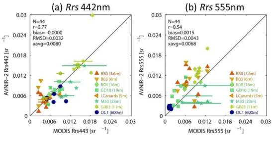
The comparison between AVNIR Rrs and MODIS Rrs at 442nm (or 443 nm) and 555 nm is

303

shown in Fig. 7. AVNIR-2 Rrs at 555nm appears slightly higher, but the results are closely

304

correlated (0.77 and 0.54 at 442 nm and 555 nm, respectively, and the Root Mean Square 305

Difference (RMSD) was about 40% and 63% of the average Rrs for AVNIR-2 and MODIS,

306

respectively) except for some samples at the shallow stations (e.g., B50 and B03). An outlier at 307

station G003 in Fig 7a (AVNIR-2 Rrs at 442 nm is about 0.03) seemed to be influenced by

308

cloud edge in the AVNIR-2 image on 31 Jul. 2007. 309

Figures 6e and 6j show the AVNIR-2 ρw at 463nm with the correction of bottom

310

reflectance. The correction decreases ρw inside of the lagoon (e.g., at stations M33 and G003)

311

and reduces the pattern of the bathymetry (seen Fig. 5) in most areas in the ρw images.

312

However, it seems to cause overcorrection in some areas, e.g., around the islands and the 313

barrier reef. 314

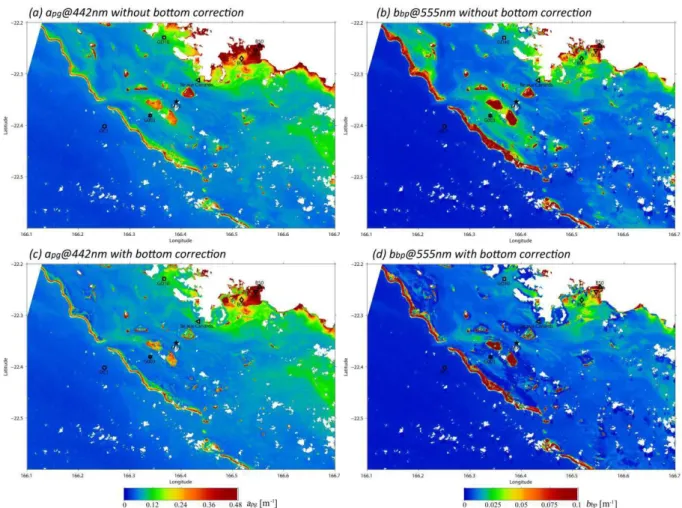
3.2 apg and bbp

315

Figures 8a and 8b shows apg at 442nm and bbp at 555nm without the bottom correction

316

(using model spectra (A) in Table 4). apg was high along the coast and in bays near the main

317

land. On the other hand, bbp was high inside the lagoon especially at shallow bottom areas (e.g.,

16 G003). Scatter plots between the in situ (ap× 1.52) and the AVNIR-2 apg and bbp estimates are

319

shown in Figs. 9a and 9b. They show that AVNIR-2 apg is well correlated with in situ values

320

for apg (r = 0.91 in Fig. 9a) even though the factor 1.52 may vary with changing proportions of

321

ap or ag in apg = ap + ag. AVNIR-2 bbp showed a high correlation coefficient (about 0.94 at 555

322

nm), but some values of bbp were higher than the in situ bbp. The overestimated samples were

323

found in shallow areas (3.6 m, 6 m, 5m, and 11 m at stations B50, B03, Ile aux Canards and 324

G003 respectively). 325

Figures 8c and 8d show apg and bbp with the bottom reflectance correction on 3 Sep 2009.

326

The correction decreased apg and bbp in the lagoon areas. The comparison to the in-situ

327

observations (Figs. 9c and 9d) showed that the correction improved the agreement especially at 328

stations M33, Ile aux Canards, and G003 where the bottom depth is shallow and apg is

329

relatively low. The AVNIR-2 apg was still higher than the in-situ apg at stations B50 and B03

330

around the Boulari Bay. Bias of apg (bbp) were improved from 0.188 to 0.118 (from 0.023 to

331

0.015), and RMSD of apg (bbp) from 0.489 to 0.290 (from 0.042 to 0.025) by the bottom

332

correction. 333

Table 4 shows the results for the fifteen match-ups by using different spectra of apg and bbp.

334

Superscripts − and + show results with smaller or larger bias or RMSD (statistically 335

significance level of 95%) than ones by the model spectrum (A). The results depended on the 336

model spectra significantly, and the model (D) brought the smallest RMSD of both apg and bbp

337

with the bottom reflectance correction. Note that the microplankton for aph [58] gives larger

338

RMSD than the measured around New Caledonia. Similarly, a slope of Y = −2 is too different 339

from those measured and would not allow a proper retrieval of IOPs from AVNIR-2. Figures 340

17 9e-9h show the scatter plots by the model spectrum (D). RMSDs of apg and bbp are significantly

341

decreased (especially stations B50 and B03) by the optimal model spectrum. 342

3.3 Chlorophyll-a concentration

343

Figures 10 and 11 show the comparison among Chla estimated from apg (by the optimal

344

model (D)), Chla calculated by OC2M-HI (using Rrs by AVNIR-2), and the MODIS standard

345

(OC3M) 1-km Chla. Chla estimated from apg (Figs. 10a and 11a) was slightly smaller than

346

Chla determined by other algorithms in the lagoon areas (e.g., sites B08 and Ile aux Canards in 347

Figs. 10 and 11). The AVNIR-2 OC2M-HI Chla was larger than indicated by the in situ data 348

and similar to the MODIS standard value in the lagoon (see around sites M33 and G003 in Figs. 349

10b, 10e, and Figs. 11b and 11e). The scatter plots show that Chla from apg provides the best

350

agreement among the three methods in the lagoon (RMSD=0.47, 0.61, and 0.60 in Figs. 10a, 351

10b, and 10e). The MODIS data at stations M33 and GD10 were scattered because they were 352

too near the coast or the lagoon islands compared to the 1-km resolution products. 353

Figures 11c and 11d show results with the bottom correction. OC2M-HI Chla (Fig. 11d) 354

was calculated by Rrs from rrsdp (Eq. (8)). Usual high biases of apg and bbp in the shallow areas

355

(B50, B03, and Ile aux Canards) around lagoon islands were decreased by the correction (Figs. 356

8c and 8d). It reduced overestimate of Chla by both apg and OC2 schemes, and improved the

357

agreement with the in-situ matchups inside the lagoon (Figs. 10c and 10d). 358

18

4. DISCUSSION

359

4.1 apg and bbp spectra

360

Agreement with in situ data was dependent on spectra of apg and bbp (Table 4). For example,

361

the aph spectrum of microplankton [58] (model C) and bbp spectrum of Y=−2.0 (F) caused

362

worse results than the spectrum modeled from New Caledonia in situ measurements (A) (Table 363

4). The agreement may be improved further if we optimize the spectra to more specific water 364

types, e.g., bays near the main land, middle-lagoon waters, and waters outside of the barrier 365

reef (e.g., open ocean). For example, modification of spectral slope of adg improved the IOP

366

estimate especially around the Boulari Bay (model (D) in Fig. 9). The accuracies of the best 367

results (r=0.91 and r=0.75 in Figs. 9g and 9h respectively) were better than ones by Quasi-368

Analytical Algorithm (QAA) [52,64] by using 1km MODIS Aqua Rrs data (r=0.84 and 0.72 369

for apg 443nm and bbp 555nm respectively (Figures of QAA results are not shown here).

370

Such an optimization with the best-candidate spectra can be a useful way to obtain locally-371

optimized environmental monitoring from satellite observations with theoretical understanding 372

of the local optical environment. 373

This study cannot determine spectral models such as the ratio between ap and ag (or aph and

374

adg), because AVNIR-2 has only two channels in the blue and green wavelengths. More bands

375

at 250 m to 300 m of spatial resolution from sensors such as SGLI and OLCI may be able to 376

improve the discrimination of the IOPs. 377

The IOP retrieval schemes have been developed for observations by narrow (about 10-378

20nm) band-width sensors, estimates of absorption coefficients by the wide band can cause 379

errors reaching about 20% [65] by the QAA [52,64] through the integration of the IOP spectra 380

19 in the band wavelengths. Our estimates rely on relatively wide bands (about 90nm) of AVNIR-381

2. We confirmed our retrieval of apg by the LMI can change about 20% (mostly overestimated)

382

using simulated Rrs from our in-situ apg and bbp. The error is still much smaller than the error

383

due to difference of the model IOP spectra, however, it will need to be considered for more 384

precise estimate in the future. 385

4.2 Aerosol and sea surface reflection estimation

386

Most of the iteration schemes for the atmospheric correction use the relationship between 387

NIR Rrs and Chla. This study uses the relationships among apg, bbp, ρag, and α based on the

388

convergence of bbp. This scheme can avoid negative IOPs by tuning the aerosol parameters α

389

and ρag in the iteration process. Another merit of this aerosol estimation is the fast processing

390

time (2-3 minutes for our study area (2001×1334 pixels) by a wide-use PC Linux machine) 391

because it does not require time to access the aerosol look-up table that is used in the standard 392

ocean color atmospheric correction algorithms. 393

The New Caledonia lagoon area has a relatively clear atmosphere compared to coasts in the 394

northern hemisphere, such as the Asian coasts. This scheme does not consider absorptive 395

aerosols that cannot be described by the simple Eq. (3). For more complex atmosphere 396

(aerosol) conditions, more bands may be necessary than the two that were used here for the 397

aerosol characterization (this study used 652 nm and 821 nm). If the sensor has lower noise and 398

SWIR bands (e.g., MODIS 500 m bands and SGLI 250m band), we may be able to estimate α 399

at each pixel and obtain more realistic measurements of α and ρag. However, the absorptive

400

aerosol correction may still be difficult using the simple Eq. (3). 401

20

4.3 The bottom effect

402

AVNIR-2 bbp seemed to be influenced by the bottom reflectance. Bottom sands can be seen

403

from satellite if bathymetry is shallow. For example, the bottom depth of the station G003 is 11 404

m with a relatively low apg. Agreement between AVNIR-2 IOPs and in situ IOPs were

405

improved by considering the bottom reflectance generally, but they seemed to be overcorrected 406

in some areas around the islands and along the barrier reef (Fig 6j). They are supposed to be 407

influenced by coverage of live corals or sediment from the land, which may cause a different 408

spectrum of the bottom reflectance from the coral sand reflectance [60,61,62]. This indicates 409

that our IOP estimation could be improved if the precise bottom depth and real bottom 410

reflectance are used [36]. 411

4.4 Cloud shadow and adjacent scattering

412

For the 10-m resolution data, it is important to consider cloud shadow and sea surface 413

reflection of scattered light from the cloud bottom. Identification of clouds around the coast 414

(including over the land) and geometric calculation considering the cloud height are required. 415

In addition, the clouds and land area can influence the coastal ocean color estimation, which is 416

known as the adjacent effect [66]. The influence of the cloud shadow seemed to affect bbp, but

417

not apg as observed in the southeastern part of Fig. 8. Further study is needed to determine bbp

418

in the absence of the influence of the cloud effects. 419

5. CONCLUSION

420

This study investigated the correction of atmospheric scattering and sea surface reflection 421

in the southwest region of the New Caledonia lagoon using AVNIR-2 images, which have four 422

bands from visible to NIR wavelengths with 10-m resolution (our processing was conducted 423

21 after averaging for 30-m (3×3) grids). We applied corrections for gas absorption, molecule 424

scattering, and ρa + ρg using the iteration scheme for converging bbp through IOPs from visible

425

bands. This scheme was able to correct fine structure patterns of the ρa + ρg successfully. The

426

AVNIR-2-estimated Rrs agreed well with the MODIS Rrs (root-mean square difference /

427

average of Rrs at 443 nm = 40%). Future projects, e.g., the Global Change Observation Mission

428

(GCOM), using the Second-generation Global Imager (SGLI) and the Sentinel-3 Ocean and 429

Land Colour Imager (OLCI), will have finer (250 m - 300 m) spatial resolution aiming for 430

coastal monitoring with a swath of more than 1150 km. These missions will require a 431

correction of the surface reflection with high spatial resolution and a reduction of masked areas 432

in order to increase the observation frequency in the coastal areas. 433

With the bottom correction, the AVNIR-2-estimated IOPs agreed well with in situ IOP 434

measurements (correlation coefficients were more than 0.9). Overcorrection appeared in the 435

muddy bays and along the barrier reef, and it suggested that a constant bottom reflectance was 436

not applicable in these areas. 437

This study showed that the AVNIR-2-estimated Chla from the apg regression scheme in the

438

lagoon area does not show the overestimation observed with the blue / green Rrs ratio. This

439

also confirms that the relationship between Chla and apg in the lagoon area is not different from

440

the apg-Chla relationship of the NOMAD database as already shown in [27]. The NOMAD

441

relationship cannot be used in bays (e.g., B50), where the apg-Chla relationship is disturbed by

442

absorbing mineral particles and irregular ag due to river discharge.

443

Our atmospheric correction and IOP estimation scheme which requires only four bands in 444

the visible and NIR wavelengths can be applied to other satellite sensors, such as the MODIS 445

22 500-m bands, and other multi-band sensors, such as SGLI 250-m bands. The performance 446

depends on the candidate spectra of IOPs based on in situ measurements (and aerosols) in the 447

target areas. This reinforces the need to construct databases of the various spectra of IOPs and 448

aerosols in various regions through international collaboration to develop globally applicable 449

approaches. The target of this study is not to make a fixed algorithm, but demonstrate the 450

method to make local optimal estimate of the IOPs and Chla. So, the algorithm should not be 451

applied elsewhere without a similar effort i.e., preparation of the candidate spectra for the 452

target areas. 453

ACKNOWLEDGEMENTS

454

The authors are grateful to the OpenCLASTR project and the NIES GOSAT project for the use 455

of the Rstar6b and Pstar2b packages in this research. MODIS L2 Rrs and chlorophyll-a data

456

were provided by NASA OBPG. OMI ozone data were provided by the Goddard Space Flight 457

Center. NCEP wind speed and sea level pressure data were provided by the NCEP/NCAR 458

Reanalysis Project. ALOS AVNIR-2 data were provided by the JAXA EORC ALOS research 459

and application project. In situ data were obtained in the frame of INSU PNTS ValHyBio and 460

processed using the SeaDAS and home package. The apg-Chla relationship was calculated

461

using NOMAD Version 2.0 ALPHA, which was compiled by the NASA OBPG, Goddard 462

Space Flight Center. 463

464

APPENDIX:

465

Calculation of TOA reflectance with gaseous absorption correction

23

ρt(b) = Lavnir2(b) / fvc(b) ×π× d2 /F0(b) / cos(θsun) /toz /twv /tO2 (A1)

467

where toz = exp(−koz(b) × (oz − 343.8)× pl) (A2)

468

twv = exp(−{ kwv(b) × (ptw−14.19) × pl + kwv2(b) × ((ptw×pl)2− (14.19×pl)2) } ) (A3)

469

tO2 = exp(−kO2(b) × (prs − 1013.25) × 0.2095 × pl) (A4)

470

pl = 1 / cos(θsun ) + 1 / cos(θsat ) (A5)

471

Lavnir2 is the AVNIR-2-observed radiance [W/m2/µm/sr], b represents the AVNIR-2 spectral

472

bands, fvc is the vicarious calibration factor defined as ratio of AVNIR-2 radiance to radiance

473

simulated by MODIS observation, d is the sun-earth distance [AU], F0 is the solar irradiance at

474

1 AU [67], θsun is the solar zenith angle [rad], θsat is the satellite zenith angle [rad], oz is the

475

column ozone [DU], ptw is the column water vapor [mm], and prs is the sea-level pressure 476

[hPa]. The gas absorption coefficients koz, kwv and kO2 were calculated by MODTRAN 4 [68]

477

considering the spectral response of the AVNIR-2 bands (Table 2). We used ptw and prs from 478

the National Centers for Environmental Prediction (NCEP) and oz from the Ozone Monitoring 479

Instrument (OMI), which is distributed by Goddard Space Flight Center. 480

REFERENCES

481

1. R. Frouin, M. Schwindling, and P. Y. Deschamps, “Spectral reflectance of sea foam in the 482

visible and near infrared: in situ measurements and remote sensing implications,” Journal 483

of Geophysical Research, 101, 14361-14371 (1996). 484

2. K. D. Moore, K. J.Voss, and H. R. Gordon, “Spectral reflectance of whitecaps: their 485

contribution to water-leaving radiance”, Journal of Geophysical Research, 105, 6493-6499 486

(2000). 487

24 3. J.-M. Nicolas, P.-Y. Deschamps, and R. Frouin, “Spectral Reflectance of Oceanic 488

Whitecaps in the Visible and near Infrared: Aircraft Measurements Over Open Ocean,” 489

Geophysical Reearch Letter, 28 (23), 4445-4448 (2001). 490

4. C. Cox, and W. Munk, “Measurements of the roughness of the sea surface from 491

photographs of the sun’s glitter,” Journal of the Optical Society Of America., 44, 838-850 492

(1954). 493

5. M. Wang, and S.W. Bailey, “Correction of sun glint contamination on the SeaWiFS ocean 494

and atmosphere products,” Applied Optics, 40, 4790-4798 (2001). 495

6. G.C. Feldman, “The OC2 algorithm for MODIS,” Seadas Forum, NASA-GSFC, NASA 496

OceanColor webpage http://oceancolor.gsfc.nasa.gov/REPROCESSING/R2009/. 497

7. E. Hochberg, S. Andrefouet, and M. Tyler, “Sea Surface Correction of High Spatial 498

Resolution Ikonos Images to Improve Bottom Mapping in Near-Shore Environments,” 499

IEEE Trans. Geosci. Remote Sens., 41, 1724-1729 (2003). 500

8. J. A. Goodman, Z-P. Lee, and S. L. Ustin, “Influence of Atmospheric and Sea-Surface 501

Corrections on Retrieval of Bottom Depth and Reflectance Using a Semi-Analytical 502

Model: A Case Study in Kaneohe Bay, Hawaii,” Appl. Optics, 47, F1-F11 (2008). 503

9. H. Murakami, and R. Frouin, “Correction of sea surface reflection in the coastal area,” 504

Proc. SPIE Vol. 7150-4, Remote Sensing of Inland, Coastal, and Oceanic Waters edited by 505

R. Frouin, Proc. SPIE Asia-Pacific Remote Sensing, 17-21 November 2008, Nouméa, New 506

Caledonia (2008). 507

10. R. Fichez, L. Breau, C. Chevillon, S. Chifflet, P. Douillet, V. Faure, J.M. Fernandez, P. 508

Gérard, L. Hédouin, A. Lapetite, S. Ouillon, O. Pringault, and J.P. Torréton, “Origine, 509

25 transport et devenir des apports naturels et anthropiques dans le lagon sud-ouest de 510

Nouvelle-Calédonie,” Journal de la Société des Océanistes, 126-127, 41-58 (2008). 511

11. R. Fichez, S. Chifflet, P. Douillet, P. Gerard, F. Gutierrez, A. Jouon, S. Ouillon, and C. 512

Grenz, “Biogeochemical typology and temporal variability of lagoon waters in a coral reef 513

ecosystem subject to terrigeneous and anthropogenic inputs (New Caledonia),” Marine 514

Pollution Bulletin, 61, 7-12, 309-322 (2010). 515

12. S.Ouillon, P.Douillet, J.P. Lefebvre, R. Le Gendre, A. Jouon, P. Bonneton, J.M. Fernandez, 516

C. Chevillon, O. Magand, J. Lefevre, P. Le Hir, R. Laganier, F. Dumas, P. Marchesiello, A. 517

Bel Madani, S. Andrefouet, J.Y. Panche, and R. Fichez, "Circulation and suspended 518

sediment transport in a coral reef lagoon: the southwest lagoon of New Caledonia," Marine 519

Pollution Bulletin, 61, 7-12, 269-296 (2010). 520

13. J.Lefèvre, P. C. Marchesiello, N. C. Jourdain, C. Menkes, and A. Leroy, “Weather 521

regimes and orographic circulation around New Caledonia,” Marine Pollution Bulletin, 61, 522

413-431 (2010). 523

14. R.Fuchs, C. Dupouy, P. Douillet, F. Dumas, M. Caillaud, A. Mangin, and C. Pinazo, 524

“Modelling the impact of a La Niña event on a South West Pacific Lagoon,” Marine 525

Pollution Bulletin (2012) in press. 526

15. J. Neveux, M.M.B. Tenorio, S. Jacquet, J.-P. Torreton, P. Douillet, S. Ouillon, and C. 527

Dupouy, “Chlorophylls and phycoerythrins as markers of environmental forcings 528

including cyclone Erica effect (March 2003) on phytoplankton in the southwest lagoon of 529

New Caledonia and oceanic adjacent area,” International J. Oceanogr., Article ID 23251, 530

doi:10.1155/2009/232513 (2009). 531

26 16. J.P. Torréton, E. Rochelle-Newall, O. Pringault, S. Jacquet, V. Faure, E. Briand, 532

“Variability of primary and bacterial production in a coral reef lagoon (New Caledonia),” 533

Mar Pollut Bull, 61, 335-348 (2010). 534

17. C. Dupouy, G. Dirberg, J. Neveux, M. Tenorio, and A. Le Bouteiller, “The contribution of 535

Trichodesmium to inherent optical properties of a tropical oligotrophic archipelago,” in: 536

Conference CD-ROM ‘‘OCEAN OPTICS XVII”, 26 October–3 November 2004, 537

Fremantle, Australia, 3pp (2004). 538

18. C. Dupouy, D. Benielli-Gary, Y. Dandonneau, J. Neveux, G. Dirberg, and T. Westberry, 539

“On the feasibility of detecting Trichodesmium blooms with SeaWiFS in the South 540

Western Tropical Pacific,” Remote Sensing of Inland, Coastal, and Oceanic Waters. 541

Proceedings of SPIE, vol. 7150. SPIE, Bellingham, WA [7150 37] 715010, 9pp (2008). 542

19. C. Dupouy, J. Neveux, G. Dirberg, M.M.B. Tenorio, R. Rottgers, and S. Ouillon, “Bio-543

optical properties of marine cyanobacteria Trichodesmium, spp.,” Journal of Applied 544

Remote Sens. 2, 023503 (2008). 545

20. C. Dupouy, D. Benielli-Gary, J. Neveux, Y. Dandonneau, and T. Westberry, “A new 546

algorithm for detecting Trichodesmium surface blooms in the South Western Tropical 547

Pacific,” Biogeosciences, 8, 1-17 (2011). 548

21. A. Ganachaud, A. Vega, M. Rodier, C. Dupouy, C. Maes, P. Marchesiello, G. Eldin, K. 549

Ridgway, and R. Le Borgne, “Observed impact of upwelling on water properties and 550

biological activity off the southwest coast of New Caledonia,” Marine Pollution Bulletin, 551

61, 449-464 (2010). 552

22. J. Neveux, J.-P. Lefebvre, R. Le Gendre, C. Dupouy, F. Gallois, C. Courties, P. Gerard, S. 553

Ouillon, and J.M. Fernandez, “Phytoplankton dynamics in New-Caledonian lagoon during 554

27 a southeast trade winds event,” Journal Marine Systems, 82, 230-244, doi:10.1016/ 555

j.jmarsys.2010.05.010 (2010). 556

23. C. Dupouy, A. Minghelli-Roman, M. Despinoy, R. Röttgers, J. Neveux, S. Ouillon, C. 557

Pinazo, and M. Petit, “MODIS/Aqua chlorophyll monitoring of the New Caledonia 558

lagoon: the VALHYBIO project,” in Proceedings of SPIE, Vol. 7150 (SPIE, Bellingham, 559

WA, 2008) [7150 41] 715014, 8 pp (2008). 560

24. R. Fuchs, C. Pinazo, P. Douillet, C. Dupouy, and V. Faure, “New Caledonia Surface 561

lagoon chlorophyll modeling as coastal reef area health indicator,” in “Remote sensing of 562

the coastal ocean, land, and atmosphere environment“ edited by Robert J. Frouin, Proc. 563

SPIE Vol. AE103 (SPIE, Bellingham, WA, 2010) [7858 20], 9 pp (2010). 564

25. M. Babin, D. Stramski, G.M. Ferrari, H. Claustre, A. Bricaud, and G. Obolenski, 565

“Variations in the light absorption coefficients of phytoplankton, non-algal particles, and 566

dissolved organic matter in coastal waters around Europe," Journal of Geophysical 567

Research, 108. doi:10.1029/2001JC000882 (2003). 568

26. C.M. Hu, Z.Q. Chen, T.D. Clayton, P. Swarzenski, J.C. Brock, and F.E. Muller-Karger, 569

“Assessment of estuarine water-quality indicators using MODIS medium resolution bands: 570

initial results from Tampa Bay, FL.,” Remote Sensing of Environment, 93, 423–441 (2004). 571

27. C. Dupouy, J. Neveux, S. Ouillon, R. Frouin, H. Murakami, S. Hochard, and G. Dirberg, 572

“Inherent optical properties and satellite retrieval of chlorophyll concentration in the 573

lagoon and open ocean waters of New Caledonia,” Marine Pollution Bulletin 61, 503–518, 574

doi:10.1016/j.marpolbul.2010.06.039 (2010). 575

28 28. J.G. Acker, A. Vasilkov, D. Nadeau, and N. Kuring, “Use of SeaWiFS ocean color data to 576

estimate neritic sediment mass transport from carbonate platforms for two hurricane-577

forced events,” Coral Reefs, 23, 39–47 (2004). 578

29. D. Blondeau-Patissier, V.E. Brando, K. Oubelkheir, A.G. Dekker, L.A. Clementson, and P. 579

Daniel, “Bio-optical variability of the absorption and scattering properties of the 580

Queensland inshore and reef waters, Australia,” Journal of Geophysical Research, 114, 581

C05003,doi:10.1029/2008JC005039 (2009). 582

30. K. Oubelkheir, L.A. Clementson, I.T. Webster, P.W. Ford, A.G. Dekker, L.C. Radke, and 583

P.Daniel, “Using inherent optical properties to investigate biogeochemical dynamics in a 584

tropical macrotidal coastal system,” Journal of Geophysical Research, 111, C07021 585

doi:10.1029/2005JC003113 (2006). 586

31. S. Ouillon, P. Douillet, A. Petrenko, J. Neveux, C. Dupouy, J.-M. Froidefond, S. 587

Andréfouët, and A. Muñoz-Caravaca, “Optical Algorithms at Satellite Wavelengths for 588

Total Suspended Matter in Tropical Coastal Waters,” Sensors, 8, 4165-4185; doi: 589

10.3390/s8074165 (2008). 590

32. C. Dupouy, and R. Roettgers, “Absorption by different components during a high 591

freshwater event of the 2008 La Nina episode in a tropical lagoon,” Poster Session “Bio-592

optics and biogeochemistry”, Ocean Optics XX, Anchorage (Alaska), 25-30 September 593

2010 (2010). 594

33. Z-P. Lee, K.L. Carder, R.F. Chen, and T.G. Peacock, “Properties of the water column and 595

bottom derived from Airborne Visible Infrared Imaging Spectrometer (AVIRIS) data,” 596

Journal of Geophysical Research, 106, 11639–11651 (2001). 597

29 34. J.P. Cannizaro, and K.L. Carder, “Estimating chlorophyll a concentrations from remote-598

sensing reflectance in optically shallow waters,” Remote Sensing of Environment, 101, 13– 599

24 (2006). 600

35. A. Minghelli-Roman, L. Polidori, S. Mathieu-Blanc, L. Loubersac, and F. Cauneau, 601

“Bathymetric estimation using MeRIS images in coastal sea waters,” IEEE Transactions 602

Geosciences Remote Sensing, 4, 274–277 (2007). 603

36. A. Minghelli-Roman, C. Dupouy, C.Chevillon, P. Douillet, “Bathymetry retrieval and sea 604

bed mapping in the lagoon of New Caledonia with MeRIS images,” in Proceedings SPIE, 605

7858 (SPIE, Bellingham, WA, 2010) [78580Y (Nov. 3, 2010)], 7 pp., doi: 606

10.1117/12.870729 (2010). 607

37. S. Andréfouët, M. J. Costello, M. Rast, and S. Sathyendranath, “Preface: Earth 608

observations for marine and coastal biodiversity and ecosystems,” Remote Sensing of 609

Environment, 112, 3297–3299 (2008). 610

38. C. Dupouy, T. Savranski, J. Lefevre, M. Despinoy, M. Mangeas, R. Fuchs, S. Ouillon, and 611

M. Petit, “Monitoring chlorophyll of the South West Tropical Pacific,” Communication at 612

the 34th International Symposium on Remote Sensing of Environment, Sydney, 10-14 613

April 2011 (2011). 614

39. C. Dupouy, G. Wattelez, R. Fuchs, J. Lefèvre, M. Mangeas, H. Murakami, and R. Frouin, 615

“The colour of the Coral Sea,” In Proceedings of the 12th International Coral Reef 616

Symposium, 18E– The future of the Coral Sea reefs and sea mounts, Cairns, Australia, 9-617

13 July 2012, ICRS2012_18E-2 (2012). 618

30 40. T. Tadono, M. Shimada, H. Murakami, T. Hashimoto, J. Takaku, A. Mukaida, and S. 619

Kawamoto, “Initial results of calibration and validation for PRISM and AVNIR-2,” Asian 620

Journal of Geoinformatics, 6, 4, 11–20 (2006). 621

41. H. Murakami, T. Tadono, H. Imai, J. Nieke, and M. Shimada, “Improvement of AVNIR-2 622

radiometric calibration by comparison of cross-calibration and on-board lamp calibration,” 623

IEEE TGRS, 47, 12, pp. 4051-4059 (2009). 624

42. F.E. Hoge, and P.E. Lyon, “Satellite retrieval of inherent optical properties by linear 625

matrix inversion of oceanic radiance models: an analysis of model and radiance 626

measurement errors,” Journal of Geophysical Research, 101, 16631-16648 (1996). 627

43. F.E. Hoge, and P.E. Lyon, “Spectral parameters of inherent optical property models: 628

Methods for satellite retrieval by matrix inversion of an oceanic radiance model,” Applied 629

Optics, 38, 1657-1662 (1999). 630

44. P. Lyon, and F. Hoge, “The Linear Matrix Inversion Algorithm,” Chap. 7 of IOCCG 631

Report Number 5, Remote Sensing of Inherent Optical Properties: Fundamentals, Tests of 632

Algorithms, and Applications, Ed. by Z. Lee (2006). 633

45. Y. Ota, A. Higurashi, T. Nakajima, and T. Yokota, “Matrix formulations of radiative 634

transfer including the polarization effect in a coupled atmosphere-ocean system,” Journal 635

of Quantitative Spectroscopy and Radiative Transfer, Vol. 111-6, 878-894 (2010). 636

46. T. Nakajima, and M. Tanaka, “Matrix formulation for the transfer of solar radiation in a 637

plane-parallel scattering atmosphere,” J. Quantitative Spectroscopic Radiative Transfer, 35, 638

13-21 (1986). 639

31 47. T. Nakajima, and M. Tanaka, “Algorithms for radiative intensity calculations in 640

moderately thick atmospheres using a truncation approximation,” Journal of Quantitative 641

Spectroscopic Radiative Transfer, 40, 51-69 (1988). 642

48. K. Stamnes, S.-C. Tsay, W. Wiscombe, and K. Jayaweera, “Numerically stable algorithm 643

for discrete-ordinate-method radiative transfer in multiple scattering and emitting layered 644

media,” Applied Optics, 27, 2502-2509 (1988). 645

49. R. Frouin, P-Y. Deschanmps, L. Gross-Colzy, H. Murakami, and T. Y. Nakajima, 646

“Retrieval of Chlorophyll-a Concentration via Linear Combination of ADEOS-II Global 647

Imager Data,” Journal of Oceanography, 62, 331-337 (2006). 648

50. R. Zaneveld, A. Barnard, and Z-P. Lee, “Why area Inherent Optical Properties Needed in 649

Ocean-Colour Remote Sensing?,” Chap. 1 of IOCCG Report Number 5, Remote Sensing 650

of Inherent Optical Properties: Fundamentals, Tests of Algorithms, and Applications, Ed. 651

by Z. Lee (2006). 652

51. H.R. Gordon, O.B. Brown, R.H. Evans, J.W. Brown, R.C. Smith, K.S. Baker, and D.K. 653

Clark, “A semi-analytic radiance model of ocean color,” Journal of Geophysical Research, 654

93 (D9), 10909–10924 (1988). 655

52. Z-P. Lee, K.L. Carder, and R. A. Arnone, “Deriving inherent optical properties from water 656

color: a multiband quasi-analytical algorithm for optically deep waters,” Applied Optics, 657

41, 5755-5772 (2002). 658

53. R.M. Pope, and E.S. Fry, “Absorption spectrum (380-700 nm) of pure water. II. 659

Integrating cavity measurements,” Applied Optics,36, 8710-8723 (1997). 660

54. L. Kou, D. Labrie, and P. Chylek, “Refractive indices of water and ice in the 0.65-2.5 µm 661

spectral range,” Applied Optics, 32, 3531-3540 (1993). 662

32 55. P.J. Werdell, and S.W. Bailey, “An improved bio-optical data set for ocean color algorithm 663

development and satellite data product validation,” Remote Sensing of Environment, 98, 664

122-140 (2005). 665

56. C. Dupouy, J. Neveux, and J.M. Andre, “Spectral absorption coefficient of 666

photosynthetically active pigments in the equatorial Pacific Ocean (165°E–150°W),” Dee-667

p Sea Research, Part II, 44, 1881–1906 (1997). 668

57. J. Neveux, and F. Lantoine, “Spectrofluorometric assay of chlorophylls and pheophytins 669

using the least squares approximation technique,” Deep-Sea Research, Part I, 40, 1747– 670

1765 (1993). 671

58. A.M. Ciotti, M.R. Lewis, and J.J. Cullen, “Assessment of the relationships between 672

dominant cell size in natural phytoplankton communities and spectral shape of the 673

absorption coefficient,” Limnology and Oceanography, 4, 404-417 (2002). 674

59. Z-P. Lee, K.L. Carder, C.D. Mobley, R.G. Steward, and J. S. Patch, “Hyperspectral remote 675

sensing for shallow waters: 2. Deriving bottom depths and water properties by 676

optimization,” Applied Optics, 38, 3831-3843 (1999). 677

60. S. Maritorena, A. Morel, and B. Gentili, “Diffise reflectance of oceanic shallow waters: 678

Influence of water depth and bottom albedo,” Limnol. Oceanogr., 39(7), 1689-1703 (1994). 679

61. S. Ouillon, Y. Lucas, and J. Gaggelli, “Hyperspectral detection of sand,” In, Proc. 7th Int. 680

Conf. Remote Sensing for Marine and Coastal Environments, Veridian, Miami, 20-22 May 681

2002 (2002). 682

62. S. J. Purkis, and R. Pasterkamp, “Integrating in situ reef-top reflectance spectra with 683

Landsat TM imagery to aid shallow-tropical benthic habitat mapping,” Coral Reefs, 23, 5– 684

20 (2004). 685

33 63. B. A. Franz, “Methods for Assessing the Quality and Consistency of Ocean Color Products, 686

“ http://oceancolor.gsfc.nasa.gov/REPROCESSING/R2009/validation/ (2005). 687

64. Z. P. Lee, A. Weidemann, J. Kindle, R. Arnone, K. L. Carder, and C. Davis, “Euphotic 688

zone depth: Its derivation and implication to ocean-color remote sensing,” J. Geophys. Res. 689

112, C03009 (2007). 690

65. Z. P. Lee, “Applying narrowband remote-sensing reflectance models to wideband data”, 691

Applied Optics, 48, 3177-3183 (2009). 692

66. R. Frouin, P-Y. Deschamps, and F. Steinmetz, “Environmental effects in ocean color 693

remote sensing,” Proc. SPIE, Ocean Remote Sensing: Methods and Applications, Robert J. 694

Frouin, Editors, 745906 Vol. 7459, doi:10.1117/12.829871 (2009). 695

67. G. Thuillier, M. Hersé, D. Labs, T. Foujols, W. Peetermans, D. Gillotay, P.C. Simon, and 696

H. Mandel, “The Solar Spectral Irradiance from 200 to 2400 nm as Measured by the 697

SOLSPEC Spectrometer from the Atlas and Eureca Missions,” Solar Physics, 214, 1, 1-22 698

(2003). 699

68. A. Berka, G. P. Anderson, L. S. Bernstein, P. K. Acharya, H. Dothe, M. W. Matthew, S. M. 700

Adler-Golden, J. H. Jr.Chetwynd, S. C. Richtsmeier, B. Pukall, C. L. Allred, L. S. Jeong, 701

and M. L. Hoke, “MODTRAN4 radiative transfer modeling for atmospheric correction,” 702

Proc. SPIE Vol. 3756, p. 348-353, Optical Spectroscopic Techniques and Instrumentation 703

for Atmospheric and Space Research III, Allen M. Larar; Ed. (1999). 704

705 706