HAL Id: hal-02422526
https://hal.archives-ouvertes.fr/hal-02422526
Submitted on 22 Dec 2019
HAL is a multi-disciplinary open access
archive for the deposit and dissemination of
sci-entific research documents, whether they are
pub-lished or not. The documents may come from
teaching and research institutions in France or
abroad, or from public or private research centers.
L’archive ouverte pluridisciplinaire HAL, est
destinée au dépôt et à la diffusion de documents
scientifiques de niveau recherche, publiés ou non,
émanant des établissements d’enseignement et de
recherche français ou étrangers, des laboratoires
publics ou privés.
classifier training
François Bremond, Remi Trichet
To cite this version:
François Bremond, Remi Trichet. How to train your dragon: best practices in pedestrian classifier
training. IEEE Access, IEEE, 2019, pp.3527-3538. �10.1109/ACCESS.2019.2891950�. �hal-02422526�
How to train your dragon: best practices in
pedestrian classifier training
Remi Trichet, [email protected] Francois Bremond, [email protected]
Abstract—The present year witnesses another milestone in
Pedestrian detection’s journey: it has achieved remarkable pro-gresses in the course of the past 15 years, and experts foresee an everyday use of numerous stemming applications within the next 15. Standing on the tipping point between yesterday and tomorrow pushes to the field’s retrospect. Features, context, the combination of approaches, and feature data are responsible for most of the breakthroughs in pedestrian detection. If the first three elements cover the bulk of the literature, much less efforts have been dedicated to feature data. In many aspects, the construction of a training set remains similar to what it was at the birth of the domain, some related problems are not well studied, and sometimes still tackled empirically. This paper gets down to the study of pedestrian classifier training conditions. More than a survey of existing training classifiers or features, our goal is to highlight impactful parameters, potential new research directions, and combination dilemmas. Our findings are experimentally verified on two major datasets: the INRIA and Caltech-USA datasets.
Index Terms—pedestrian detection, real-time, data selection,
parameter estimation, big data, dataset training
I. INTRODUCTION
Accurately detecting human beings in an image is a task that an infant can perform at the age of one, but a computer algorithm still can’t reliably achieve. Nevertheless, a wide range of applications such as congestion analysis, automotive, abnormal event detection, retail data mining, robotics, human gait characterization have boosted the field’s progresses which is now at the core of many computer vision advances.
In a recent study [5], features, context, feature data, and the combination of approaches have been identified as the key performance elements for pedestrian detection. Roughly 30% of approaches focus on developing, combining or adapting fea-tures, and this direction has lead to most of the breakthroughs over the past years, such as channel features [18], or con-volutional network [47]. Context adaptation [28], harnessing frequent geometry [32][50] or environment patterns [48][64], also successfully received attention from the community, but this algorithm adaptation is often application or even dataset dependent.
However, less progress has been stated concerning other areas such as feature data, threshold estimation, or non-maximum suppression. Training sets are still generated by applying the same techniques than a decade ago: Increasing the data variability is done by blindly mixing datasets [5], and Bootstrapping [16][25] remains among the preferred choices for training set generation. To the best of our knowledge, alternatives to greedy non-maximum suppression are never considered, and the majority of training parameters are over-looked in short-length papers.
Consequently, lots of question have never been clearly answered and the related approaches are often empirical. How to augment the number of positive examples in my training set ? Is a soft-cascade always working ? What are the alternatives to non-maximum suppression ? Should we always consider data cleaning before training ? What is the best strategy to set up the classifier cascade thresholds ? These details are often understated in short-length papers. Hence, by conducting thorough parameter evaluation and comprehensive method variation tests, this detail oriented paper strives to determine what are the best practices to train a pedestrian classifier. To the best of our knowledge, these experiments are new to the community. They bring a new light on some overlooked parameters, and precise or disprove some of the community empirical findings that were never experimentally validated before.
More specifically, our contributions are manyfold. We pro-vide extensive experiments and analysis in the domains of model size, instance selection, data cleaning, data generation, as well as near real-time classifier choice and thresholding, soft-cascading, and non-maximum suppression.
In order to study underexplored state-of-the-art areas and assess parameters impact independently, we first define a base-line that performs on par with common pedestrian detectors while remaining generic enough to test on the most common competitors. To validate our experiments, we provide tests with two types of features: HoG [16] and LBP [46]; and on two major datasets, INRIA [16] and Caltech USA [20].
The rest of this paper is organized as follows. Section 2 reviews the related state-of-the-art. Section 3 describes the reference classifier training methodology along with the variants that we will utilize throughout this study. Section 4 covers the large set of experiments we have undertaken and Section 5 sums up our findings and discusses possible future directions.
II. RELATEDWORK
Classifier optimization always has been a major concern in computer vision. Techniques ranging from active learning [39] to feature augmentation [11][40] have been employed to fine-tune the classifiers on tasks as various as person re-identification [42][62][68] or event recognition [12][41].
More specifically, data selection from imbalanced datasets has been a concern for pedestrian detection since the birth of the field. [34] proved that disproportioned datasets degrade SVMs prediction accuracy, especially for non-linearly sep-arable data. Subsequent research on these experiments [65] showed that best performance was obtained for approximately
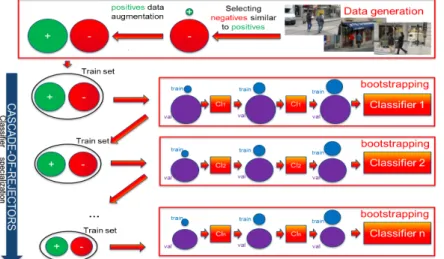
Fig. 1. Training pipeline. The initial training set generation selects data while balancing negative and positive sample cardinalities (Top). A cascade classifiers is then trained on it (Left), each independent classifier being learnt through bootstrapping (right). balanced positive and negative sets is sought all along the cascade. cl:classifier
Fig. 2. data generation example with horizontal cut. the Feature values corresponding to upper and lower body parts are concatenated to form a new data sample.
comparable class cardinalities when over-sampling the minor-ity set.
Limited work carries out these issues. Bootstrapping [16][25] is probably the most common adaptation to the problem. This data training mechanism improves accuracy thanks to successive training set updates focusing on samples difficult to classify. It is first initialized on uniformly drawn negative samples. At each iteration, the negative training set is augmented with the false positives of the previous run. The process keeps repeating until the performance converges or a memory threshold is reached. [57] further showed that 2 iterations lead to optimal performance. [27] adopted a different practice for random forest. They first train t trees with uniformly-drawn samples, use them to obtain harder positive and negative sample to train the next t trees, and iteratively repeat this process. Each tree group bears its own bias, therefore improving the overall forest performance. [24] incorporated latent values to optimise hard negative mining.
Generative techniques consider over-sampling the minority class through artificial data generation. This type of approach suffers from both, over-generalization and the risk to create erroneous data. The SMOTE algorithm [58] is probably the most renowned one. It creates new data as the linear com-bination of a randomly selected data point and one of its (same class) k nearest neighbors. Borderline-SMOTE [29] subsequently proposed to improve SMOTE through clever selection and strengthening of weak pairs. ADASYN [30] con-sidered limiting the over-generalization through density-based data generation. In the same vein, [35] introduced cluster-based oversampling, simultaneously tackling the intra- and inter-class imbalance issue. Finally, [6] proposed curriculum learning to progressively incorporate into the training set data ordered according to their generative power (i.e. from easy samples to hard ones).
Cost sensitive learning methods [22][53] are an alternative to generative techniques that learn the cost of misclassifying each data sample. They optimize the classification perfor-mance by up-weighting important data and provide a natural way to enhance the minority class.
Finally, [33] highlighted and tackled the imbalance issue with a two classifier cascade: The first one aims for a high recall whereas the second one enhances precision.
An alternate strategy to deal with the excess of negative data is to successively prune out easy-to-classify instances via the use of several consecutive classifiers. This cascade-of-rejectors [69][7] can also be considered to speed up the detection. The technique, inspired by Viola & Jones face detector [56], builds up a classifier cascade that consists of successive rejection stages that get progressively more complex, therefore rejecting more difficult candidates as the classifiers get more specialized. [52] further upgraded the principle from features to data by performing hierarchical clustering on the dataset, leading to improved classification results. However, it requires, for each new datum, to find the corresponding set of clusters it belongs to. See [31] for more details on learning from imbalanced datasets.
III. REFERENCE TRAINING METHODOLOGY The definition of a reference method is a difficult task. On one hand, it needs to be generic enough to allow the evaluation of a wide spectrum of common techniques and its reproducibility under various application environments. But on the other hand, results competitive with the state-of-the-art are required for the conclusions to be usable with up-to-date algorithms. Bearing this compromise in mind, we chose the following reference method. For the sake of conciseness, we restricted it to real-time or near real-time techniques, but in most cases, the extension to more compute-intensive strategies remain possible.
Our training methodology, illustrated in figure 1, unfolds as follows. It decomposes in two distinct parts: The initial training set generation and the classifier training. The initial training set generation carefully selects data from a set of images while balancing negative and positive sample cardinal-ities. We then train a cascade of 1 to n classifiers. This cascade could include a cascade-of-rejectors [15][69][7][52][56], a soft cascade [8], or both. In addition, each independent classifier is learnt through bootstrapping [16][25] to improve performance. One key aspect is to seek balanced positive and negative sets at all time. Hence, all along the cascade, the minority class is oversampled to create balanced positive and negative sets.
The body of this section describes each of these compo-nents independently while putting the emphasis on important
aspects or parameters that will be analysed in the next section dedicated to experiments.
A. Minority class oversampling
As the studies on the topic prove that class imbalance leads to deteriorated performance, one may seek class balance before any training. Two options exist. The first one consists in undersampling the majority class. This solution doesn’t satisfy our needs as a large training set is preferable to fully represent the data variability and avoid overfitting during the training process. The remaining solution oversamples the minority class. This process implies the creation of extra data that will not match any existing instance in the dataset images. Nevertheless, these newly created instances have to credibly represented a hypothetical data. The risk of introducing spuri-ous data in the dataset should be minimized, especially in our case, where we may generate over 90% of one class instances. Consequently, the large majority of data generation algorithms create new data by fusing the values of existing samples. In order to respect the credibility constraint, the parent data often are feature space neighbors, leading to the new data to be created in their feature space local vicinity. This is the over-generalization issue that cripples most generative techniques, like SMOTE [58]: Instead of exploring the emptiest areas of the feature space, these algorithms keep populating the denser areas, thus reinforcing the dataset biases.
In order to free the process from this issue, [55] takes advantage of the spatial localization of most pedestrian feature values. Indeed, due to their block or region decomposition, geometrically structured descriptors, such as HoG [16], LBP [1], DPM [24], or Haar-inspired strategies [18], each of their feature values have a precise localization within the proposal window. The new data generation function f (.) unfolds as follows. We randomly select 2 instances x1 = [x11, ...x1n]
and x2 = [x21, ...x2n] from the same class Si and create a
new sample with their lower and upper body features, while avoiding doublons. Uniform sampling with replacement is employed. More formally:
∀x1, x2∈ Si f (x1, x2) = [x11, ...x1n
2, x2
n
2+1, ...x2n] (1) So, a minority class of n samples can spawn a maximum of
n× (n − 1) new instances. Not normalizing the final vector
gives better results than a re-normalization.
In their approach, [55] solely used the horizontal dichotomy in order to guarantee the creation of valid data. In this paper, we choose to explore the limits of this strategy by relaxing this constraint in the experiments section.
B. Training Set Generation
This first step aims to form the initial training set by selecting insightful instances from the swarm of features extracted from the training images I. Let D be the desired training set cardinality, with training set positive and negative instances cardinality P and N so that D = P + N . To get a representative negative subset of the training set, the common approach is to randomly extract n = D/|I| data from each image. This typically leads to a large imbalanced training set
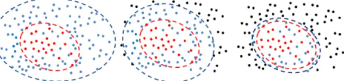
Fig. 3. Representation of the parameter n0 for instances selection. Positive
samples are in red, selected negative ones are in blue, unselected ones in black. The rough class boundaries are depicted with dashed lines. From left to right, n0=100%, n0=50%, n0=10%
with few positives P and a large subset N of negative instances. Data generation techniques [58][35] can then be employed to limit the class bias. Positive instances horizontal flipping is also frequently used.
To get a better control over the selected instances, we borrowed the strategy from [55]. In this approach, ground truth positive examples are augmented with near positives, defined as negative data having a spatial overlap with the ground truth positive samples higher than 90%. Let Pi be the
set of already selected positive data after the processing of i images. When processing image i + 1, negative samples are selected as follows:
1) Data negative samples are sorted according to their sim-ilarity with positive samples Pi.
2) Select the subset of the n0most similar negative samples
(based on euclidean distance), with n0≥ n.
3) n = D/|I| negative instances are randomly selected among the remaining subset n0.
Finally, the positive class set is oversampled to reach a balance with the negative instances.
n0 represents the overall similarity between the selected
negative N and positive data P. Setting n0low restricts the
se-lected negative data to those similar to positive ones, therefore building a classifier that focusses on the often misclassified data that lie on the border between the two classes. Inversely,
n0=100% comes back to the common approach for instance
selection where the full training set is represented. Figure 3 depicts the idea. Only ground truth positive and the same amount of original negative samples are fed to the training set, the rest of the original data and the augmented data are directed to the validation set.
C. Data cleaning
The purpose of data cleaning is to spruce the dataset off data that could potentially mislead the classifier training. In this paper, we experimented with two data cleaning methods with distinct spirits: Tomek links [54] focusses on mixed classes neighborhoods while DBSCAN cleans overpopulated areas [23].
Tomek links are defined by pairs of opposite classes data that are respective nearest neighbors. More formally, given an instance pair (xi, xj), where xi and xj are respectively
positive and negative instances, and d(xi, xj) is the distance
between xi and xj, the d(xi, xj) pair is called a Tomek link
if there is no instance xk, such that d(xi, xk) < d(xi, xj)
or d(xj, xk) < d(xi, xj). Therefore, Tomek links are drawn
either from noise, or on classes border. So they are a powerful tool, for data clean-up, especially after synthetic sampling. Tomek links can then be removed until all nearest neighbor
pairs belong to the same class. In our case, we employ euclidian distance and restrict the deletion to negative data to spare the scarce minority class.
DBSCAN cleaning makes use of the renowned density-based clustering algorithm [23]. It basically performs a density correction, removing data from the mostly populated areas of the feature space. The algorithm unfolds as follows. With number of neighbors present within distance d associated to each point, the data points are ranked according to their neighbor cardinality. The algorithm then iteratively removes the sample in the most populated neighborhood, updates the cardinalities accordingly,and stops when all data samples have less than Nmin points in their vincinity. We used the euclidian distance, d=0.8 and Nmin=5 for all our experiments.
D. Classifier
The two employed classifiers in this work are typical Adaboost [63] and random forest [9]. After specifying our random forest setting, we will remind bootstrapping, the cascade-of-rejectors and soft cascade methods in the next subsections.
In our paper, the tree construction is grounded on typical entropy optimization S: S = 1 ∑ Ci=0 −pCilog(pCi) (2)
And the final confidence score for instance x is obtained by voting: P (Ci(x)) = 1 F F ∑ t=0 ct(Ci) (3)
where F is the number of trees, ct(Ci) is the count for category
Ci at the leaf node Ltof the tthdecision tree.
E. Classifier bootstrapping
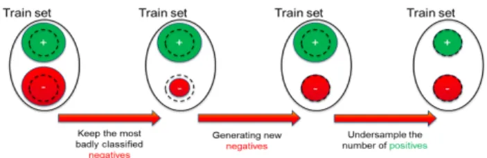
We use bootstrapping [16][25] to augment the training set. At each iteration, we incorporate the most badly classified data from the validation set into the training set and retrain the classifier. We aim to repeat this process until the training set reaches its desired initial size T .
However, a maximum of 2 iterations is advised to avoid overfitting [57]. Therefore, we employ [55] method to deal with this issue, the idea being to introduce new data to prevent overfitting. Instead of simply selecting data from the validation set, we generate it the same way as detailed in the minority class oversampling section. Each new datum is generated based on 2 data samples selected among the misclassified data. Weighted sampling is utilized in this case, the probability of an instance to be drawn being set in relation to the extent of the error. The training set reduction algorithm, illustrated in figure 4, iterates until the desired training set size is reached.
F. Cascade-of-Rejectors
The cascade-of-rejectors is an efficient strategy for siev-ing out a large proportion of false positives, and has been applied several times in the context of pedestrian detection [15][69][7][52][56]. However, tuning this cascade of classi-fiers remains problematic. First, the classiclassi-fiers are prone to
Fig. 4. Set cardinality balancing pipeline. ’+’ and ’-’ signs represent the positive and negative classes. Best viewed in color.
Fig. 5. Toy example of a cascade-of-rejectors training for binary classification. Blue and red colors represent the classes. The line depicts a (hypothetical) separating hyperplane. The first iterations optimize on recall, the final one optimizes for precision. Minority and majority classes are respectively under-and over-sampled between each iteration to learn on balanced classes. Best viewed in color.
errors that propagate along the cascade. Second, most authors employing this technique solely reject negative data after each classification step to avoid the creation of classifiers likely to reject positive data during the subsequent stages. However, this leads to progressively more imbalanced datasets. Fine tuning of the original positive versus negative instances ratio is usually necessary to obtain satisfactory results (a 2 to 4 times bigger negative set is the common practice). But this strategy is still under-optimal as balanced datasets are proved [65] to be the best performing ones.
To deal with these issues, we propose a new cascade-of-rejectors. Our approach borrows [33]’s main idea with a two-stage classification: The first one aims for a high recall whereas the second one focuses on precision.
The first stage embodies a cascade of n− 1 rejectors. To avoid increasing the false negative rate, these n− 1 initial classifiers enforce a high recall, moderately optimizing the performance on the precision. The metric formalizes as:
M = (T N× WT N+ T P )/(P + N ) (4)
with P, N, T P, T N , and WT N being respectively positive,
negative, true positive, true negative instances, and the weight associated to T N . WT Nenforces the recall. Note that WT N =
0 comes back to optimizing for recall. When WT N ≤ 0.5,
its parametrization has little impact on the results. We used
WT N = 0.5 for all our experiments. Negative data, with a
confidence below 0.5, are rejected at each stage. Negative data over-sampling is then undertaken to avoid emptying the validation set. When insufficient to match the positive instances cardinality, random positive data under-sampling is then considered. We employ Adaboost as classifiers for this part. These decision trees have demonstrated compet-itive performance whilst retaining computational efficiency [61][44]. During testing, typically over 95% of the data are safely discarded after 4-5 iterations. This cascade-of-rejectors guaranties a high recall, increased performance induced by
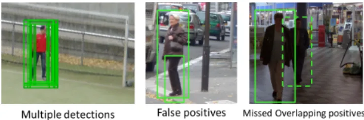
Fig. 6. Difficulties that non-maximum suppression tackles. Detections are in green. Best viewed in color.
balancing the datasets at each iteration, and few parameters to tune.
The second stage performs a finer classification, aiming for high precision results. Since the bulk of the data have been removed, more demanding computation can be performed at this stage without slowing down the detector. We employ a dense forest classifier, that has shown [5] giving slightly better performance than its counterparts on pedestrian detection. We optimize for the log-average miss rate [49]. Figure 5 illustrates the cascade effect on a toy dataset.
The only parameters that require careful tuning are the rejection thresholds t(Ci), with Ci the ith classifier of the
cascade. During ith stage of the testing cascade, any data dj with confidence Ci(dj) < t(Ci) will be rejected. Since
the method optimizes for the recall, the large majority of data around the separating border between the two classes are negative ones. It is then sensible to set t(Ci) > 0.5. See the
experiment section for a thorough evaluation of this parameter impact on performance.
G. Non-Maximum Suppression
Objects of interest generating lots of detections in their neighborhood, non-maximum suppression is a method that keeps the maxima while deleting other proposals. Its purpose is two-fold. First, aggregating the information of nearby detec-tions. It also works as an overlap control mechanism, balancing overlapping false detections and detections over self-occluding objects. Figure 6 illustrates these difficulties.
In this study, we use 3 different implementations of the threshold maximum suppression. First, Greedy non-maximum suppression is the systematically employed tech-nique that compares the bounding boxes that overlap over a pre-defined threshold and keeps the best scoring one. We set the overlap threshold to 0.6 for all our experiments. We also question its supremacy by testing out to other methods. Threshold non-maximum suppression (t-NMS) [10] groups the detection according to the bounding boxes overlap with the group best candidate, keeps the d candidates with highest confidence for each group, and builds the final candidate position with the group mean border positions. Despite its simplicity, t-NMS doesn’t require heavy parametrization and combines well with the cascade algorithms. Even though the complexity is O(n2), it is quite fast in practice since most of the negatives have already been suppressed by the cascade-of-rejectors. We set the overlap threshold to 0.4 and d = 2 for all our experiments. We also considered Scale non-maximum suppression (s-NMS) [10] that differs from t-NMS by treating each scale separately.
In the occurrence of nested detections, our parametrization always favors the biggest one. Threshold non-maximum sup-pression is utilized by default.
IV. EXPERIMENTS
This section, dedicated to our experimental validation, breaks down into several sub-parts. After presenting the datasets and the experimental setup details, we run individual experiments on each part main parameters or overlooked variations. The last part compares our work to the state-of-the-art.
A. Datasets
We experimented on the INRIA and Caltech-USA datasets. The INRIA [16] features 1832 training and 741 testing high resolution pictures. This is among the most widely used dataset for person detection. Despite its small size compared to more recent benchmarks, the INRIA dataset boasts high quality annotations and a large variety of angles, scenes, and backgrounds.
The Caltech-USA [20] dataset totals 350000 images. Despite some annotation errors [67], its large size along with crowded environments, tiny pedestrians, and numerous occlusions prob-ably make the Caltech-USA dataset the most widely used one. We experimented on the ”reasonable set” that restricts algo-rithms to pedestrians over 50 pixels in size and a maximum of 35% occlusion.
With respectively a large variability and tiny occluded detec-tions, everyday pictures and automotive application, these two datasets offer complementary settings for our experiments.
B. Experimental setup
We experimented on the INRIA [16] and Caltech-USA (reasonable set) [20] datasets with HoG [16] and Haar-LBP [14]features. HoGs are configurated with 12× 6 cells, 2 × 2 blocks and 12 angle orientations, for a total of 2640 values. Block as well as full histogram normalisation are performed. The LBP descriptor follows the same structure, features a value per channel for each cell, and non-uniform patterns are pruned out [45]. Candidates are selected using a multi-scale sliding window approach [69] with a stride of 4 pixels. Ap-proximately 60% are loosely filtered according to ”edgeness” and symmetry. No background subtraction or motion features are employed on the Caltech dataset. The training set size is up-bounded at 12K samples. Increasing this threshold doesn’t improve performance.
No generative resampling is performed. The model height is set to 100 pixels for the INRIA dataset, 50 pixels for Caltech. We also implemented a cascade-of-rejectors baseline with the commonly used settings: Rejector optimisation is done according to the log-average miss rate metric. We tested this baseline with a typical initial validation set containing 4 times more negative samples than positive ones. To compare with the common multi-dataset training technique, we also used an augmented version with PETS2009 [26] positive samples. This set gathers 50K positive instances from both datasets and 110K
Component default method default parameter Model height pixels INRIA=100 Caltech=80 # data selected FairTrain [55] INRIA=2000 Caltech=1600 Data oversampling FairTrain [55] horizontal cut Data Cleaning Tomek links
Resampling Bootstrapping 5 iterations Cascade cascade-of-rejectors 6 iterations Cascade classifier Adaboost 512 weak classifiers Cascade final classifier Adaboost 512 weak classifiers NMS t-NMS t = 0.4 and d = 2
TABLE I
DEFAULT METHODS AND PARAMETERS USED FOR THE TRAINING negatives from the sole INRIA benchmark. Table I summarizes the default methods and parameters that will be utilized for the different components alternatives.
We utilised the openCV implementation for the Adaboost and random forest classifiers. Random forest parameter set includes the number of decision trees, the number of sampled feature dimensions and the max tree depth. They were selected by measuring out-of-bag errors (OOB) [9]. It was computed as the average of prediction errors for each decision tree, using the non-selected training data. Adaboost is initialised with a tree depth of 2 and 256 weak classifiers. Each extra run adds 64 weak classifiers. This is a low number of weak classifiers compared to typical settings (i.e. [1024, 2048]). However, in practice, increasing this value leads us to lower performance and speed.
We use a variant of the threshold non-maximum suppression (t-NMS) [10] that groups the detections according to the bounding boxes overlap with the group d best candidate, keeps the d candidates with highest confidence for each group, and builds the final candidate position with the group mean border positions. We set the overlap threshold to 0.6 and d = 3 for all our experiments. Log-Average Miss Rate (LAMR) [49] is employed as metric for all runs.
C. Model size
state-of-the-art detectors empirically set the model size [49]. In this subsection, we conducted thorough experimentation to determine what should be the optimal model size given the initial conditions and what is its actual impact on performance. We varied the model height size in relation to the pedestrian minimal size observed in the dataset. We identified the smallest detections to be 50 and 60 pixels in height for respectively the Caltech (reasonable set) and INRIA datasets. And, as shown in table II, the best corresponding model sizes for these 2 benchmarks are 70 and 100 pixels in height.
The overall rule should be ”the bigger, the better” as implic-itly stated in [49]. Indeed, a bigger model will harness more information. However, the quality of the detection deteriorates when the model height size exceeds 150% of the smallest dataset pedestrian. The performance gain is then a factor of small detection frequency. As shown in [20], in Caltech’s rea-sonable set, small detections represents the bulk of occurring pedestrians whereas they remain pretty rare in INRIA, which explains the discrepancy between the two datasets.
lesson learned:Model size matters. Optimal setting is in the [m× 140%, m × 160%] range, depending on the frequency of
Model height size INRIA Caltech
m 24.61% 55.78% m× 110% 24.54% 52.82% m× 120% 23.92% 49.58% m× 130% 22.95% 47.51% m× 140% 21.44% 46.25% m× 150% 20.7% 47.73% m× 160% 20.31% 51.32% m× 170% 20.83% 57.28% m× 180% 21.34% 61.23% TABLE II
LAMRPERFORMANCE ACCORDING TO THE MODEL HEIGHT SIZE THAT IS SET IN RELATION TO THE MINIMAL PEDESTRIAN SIZEm. BEST RESULTS
IN BOLD.
the size m within the testset. When the frequency is unknown, we advise setting it up to m× 150%.
D. Instances selection
Experiments on the training set D=P+N size have been conducted in [55], with the performance reaching a plateau around 200K data instances. Therefore we will restrict our tests to the parameter n0 tuning the similarity of the selected
negative instances to the positive ones. We implemented 3 strategies for this purpose.
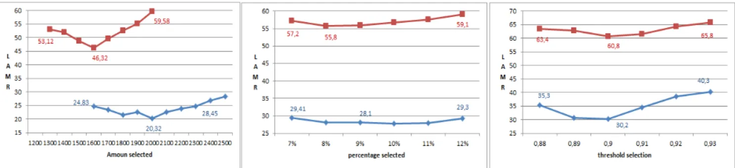
1) Percentage: Select the n0 percent most similar data.
2) Threshold: Select the data with similarity inferior to a threshold n0.
3) Amount: Select the n0 most similar data.
In every case, a minimum of n = D/m data are selected to insure the same training set cardinality. Figure 7 compares these variants performance.
Despite the rather simple strategies employed here, data selection leads to a significant classifier performance improve-ment. The best strategy clearly consists in selecting the p data most similar to positives. The other two strategies, exploring parts of the feature space further away from positive instances lead to less discriminative classifiers. We explain the lower amount of data preselected for the Caltech dataset by the lower data variability of this dataset. Indeed, the angle and commonly encountered background objects are similar over the frames.
lesson learned:data selection and adaptation is an impor-tant area that deserves more attention from the community. As shown in these experiments, careful initial instances selection is crucial, and can lead to major performance boost. The selected negatives similarity with positive data must be set in accordance to the dataset variability.
E. Data cleaning
Data cleaning is a rarely used pre-processing step. Is it overlooked or just dispensable? To answer this question, we evaluated its true importance for pedestrian training through the 2 proposed data cleaning methods. Since our training set generation method is not deterministic, each result is averaged over a total of 6 runs on the two datasets. Approximately 0.01 to 0.2% of the negative data are removed. No significant dataset discrepancy has been observed. Results are detailed in table III.
Dataset size Tomek links [54] DBSCAN [23] 80K -0.71± 0.05% -0.7± 0.13% 100K -0.85± 0.04% -0.54± 0.11% 120K -0.7± 0.1% -0.62± 0.16% 140K -0.59± 0.11% -0.34± 0.09% 160K -0.34± 0.05% -0.16± 0.07% 180K -0.19± 0.03% -0.12± 0.07% 200K -0.17± 0.05% -0.05± 0.05% TABLE III
AVERAGELAMRPERFORMANCE IMPROVEMENT INDUCED BY DATA CLEANING TECHNIQUES OVER6RUNS ON TWO DATASETS. BEST RESULTS
IN BOLD.
The use of data cleaning shows a small but steady mean improvement. Tomek links outperform DBSCAN cleaning on this experiment. We assume that the DBSCAN cleaning may remove important data on the fuzzy class borders that fine tuned training sets tend to densely populate in order to improve the classifier discriminative power. Also, its use typically counterbalances the over-generalization problem which does not impair the training set construction presented in this study (see section III-A). We also observe that the data cleaning efficiency is inversely correlated to the training set size. We assume that the repercussions of the few spurious data instances weaken in accordance to the population density in their neighbourhood.
lesson learned: If cleaning the data could be dispensable, especially for big fine tuned training sets, it never harms the classification. Counter-intuitively, the popular DBSCAN does not perform best for pedestrian detection.
F. Additional data generation
Let’s define a credible datum as a generated datum that visually looks like the object it represents. Note that the credibility of newly generated data can only be checked visually, so, the overall credibility of a generated set can hardly be quantified. In their original work, [55] restricted their data generation methodology to horizontal cuts, arguing that the newly generated instance credibility was paramount. In this experiment we test the limits of this hypothesis through the implementation of the following variations:
1) Horizontal cuts in 2 parts of equal areas. The original strategy proposed in [55]. See figure 2.
2) Vertical cuts in 2 parts of equal areas. Note that cutting along a vertical axis doesn’t equal to an instance hori-zontal flip since the two parent instances are likely to be different data.
3) Random cuts in 2 parts of equal areas. This implies the cut passing through the centre of the bounding box. Each new data will be generated according to a different cut. 4) Random walks. The first half of the blocks are selected
with the random walk algorithm [21] from the first sample. The other half of the blocks are selected from the second sample. Each new data will be generated accord-ing to a different walk. Usaccord-ing random walks guaranties that, at least, one of the 2 sets will be fully connected. 5) Random walks and horizontal cut combination. This
strategy generates negative data utilizing the random walks and positive data with horizontal cuts.
Model height size Feature INRIA Caltech Horizontal cut HoG 20.31% 46.25% Vertical cut HoG 21.28% 46.51% Random cut HoG 22.68% 48.64% Random walks HoG 25.32% 50.11% 1+4 combination HoG 22.38% 48.14% Horizontal cut LBP 18.42% 51.26% Vertical cut LBP 19.12% 52.02% Random cut LBP 20.43% 56.91% Random walks LBP 22.87% 60.89% 1+4 combination LBP 19.88% 53.28% TABLE IV
DATAGENERATION ALGORITHM ACCORDING TO4DIFFERENT STRATEGIES. SEE TEXT FOR THE DESCRIPTION OF THE METHODS. BEST
RESULTS IN BOLD.
The methods are ranked according to their generative power and the loss of credibility of the newly generated data. For instance, with the same initial set, random walks will generate a much greater variety of new data than horizontal cuts, leading to a better exploration of the feature space. However, its likelihood to create spurious data values, that doesn’t correspond to a legitimate pedestrian image is also much higher. Results are provided in table IV.
With performance inversely decreasing with the loss of newly produced data credibility, this experiment confirms that the credibility is paramount. But counter-intuitively, the same rule also applies for negative example generation that do not have this restriction. Indeed, the combination of strategies 1 and 4 doesn’t lead to any improvement. This implies that the negative samples structural geometry (i.e. a window frame, a car cabin, or tree branches) also cannot be tampered with.
lesson learned:Data generation credibility is essential and should not be jeopardized for both positive and negative instances. Horizontal cuts is the best performing method.
G. Classifier type
The general predominance of Random forest classifiers over Adaboost for pedestrian recognition have already been observed in the past [5]. In this study, We aim to push the experiment further by evaluating its actual impact within a cascade-of-rejectors. For this purpose, we tune the number of Adaboost and Random forest classifiers, keeping to 6 their total amount. Adaboost classifiers always come first in the cascade in order to benefit from their higher speed-up. This experiment is only presented for HoG features and the INRIA dataset as a similar behaviour is observed with other datasets and features.
Results are reported in table V. The only noticeable im-provement is observed when the 4 or 5 last classifiers are random forests. This is sensible as over 90% of the data have been removed after these stages and the remaining ones are mostly grouped around the pedestrians. Using random forest as first classifier doesn’t increase the results. We assume that a more discriminative classifier is less important during this first stage that focusses on negative data broadly different from the positive ones.
We also state that random forest only brings in a marginal improvement of 0.42% compared to Adaboost classifiers, contrary to what is usually reported [5][27]. We assume that
Fig. 7. Comparison of the instance selection strategy variants, setting the log-average miss rate performance in relation to the parametrization. The INRIA dataset is in red, Caltech in blue.
# Random forest classifiers INRIA Speed 0/6 20.31% 2.11fps 1/6 20.31% 1.09fps 2/6 20.29% 1.98fps 3/6 20.42% 1.75fps 4/6 20.13% 1.47fps 5/6 19.89% 1.24fps 6/6 19.92% 0.84fps TABLE V
LAMRPERFORMANCE AND SPEED OF AHOG-BASED CASCADE ON THE
INRIADATASET,WHILE VARYING THE CASCADE CLASSIFIER TYPES
(ADABOOST OR RANDOM FOREST). BEST RESULTS IN BOLD. the Adaboost and random forest performance converge with the overall result improvement.
lesson learned:Powerful classifiers perform best when used in all but first classifiers of the cascade. general progresses in the field also call back into question the random forest classifier predominance [5].
H. Soft cascade
We tested our pipeline with several variations of the famous soft-cascade [8], ranked according to their speed-up and their loss of discriminative power:
1) soft-cascade: The standard soft cascade [8] that adds one feature value at each step of the cascade.
2) block-cascade: A more discriminative but slower version of the soft cascade that adds one feature block at each step of the cascade.
3) Reverse engineering : This method Learns first the clas-sifier based on the full length descriptor and recursively removes the less discriminative half until only 2 blocks are left. It can be considered as a preprocessing step that quickly prunes out most of the negatives before running the standard cascade.
Results are presented in table VII.
Standard soft cascade provides results on par with the state-of-the-art [8], which are significantly worse than our baseline. This makes sense as classifiers trained on low feature dimen-sionality are far less discriminative than full-length descriptors. The preprocessing classifier based on reverse engineering doesn’t degrade the results but provides only a 2-fold speedup. lesson learned:These results may sound the death knell of soft-cascade. If a soft-casacade provides a huge speed boost, its classifiers are independently not discriminative enough to compete with a the most recent classifiers trained on finely selected instances.
I. Classifiers threshold setting
Training various classifiers on different data, with varying features of a classifier cascade invariably leads to a set of disparate classifiers. In addition to that, variations between train and test sets may induce more discrepancies. The use of any classifier cascade is pointless without a mechanism to cope with these variations. To deal with it, the actual strategy estimates and sets a different threshold t(Ci) for each classifier
Ci. Setting up a set of cascade thresholds is not an easy task
and the methods that tackle this particular pedestrian detection sub-problem are, at best, empirical. During testing, the optimal threshold setting is supposed to replicate the training phase dataset reduction across the cascade. In other words, each step should progressively eliminate harder negative examples while the recall should remain close or equal to 1.
In order to compare the efficacy of various commonly employed thresholding technique, we first needed to find the optimal setting. We manually looked for the threshold set leading to the best performance, exhaustively trying out all possibilities with a 0.01 step. Then, we tested the following methods:
1) Constant: Using the same threshold t(Ci) = T for each
cascade classifier t(Ci); i = 0...1
2) Increasing: Monotonously increasing the classifiers threshold. t(Ci) = T + c× 0.01.
3) Recall: Estimating thresholds during training such that recall equals to r. This is the method most commonly used in the literature.
4) Regular: Using the same purposely low threshold
t(Ci) = T for each cascade classifier t(Ci) and insuring
that d% of the remaining data are removed at each step of the cascade.
the parameter T, and d are manually set to the best per-forming value. However, the same value is employed for all datasets. T=0.58 is utilized for experiment 1, T=0.55 for experiment 2, and d=40% for experiment 4. Results are displayed in table in table VIII.
This experiment revealed several interesting points. First of all, while looking for the optimal thresholds, we stated that they are not data but feature dependent. In other words, the best threshold varies a lot when the feature dimensionality changes but remain quite similar otherwise.
Second, the most common threshold estimation strategy (3), along with the removal of a predefined amount of data at
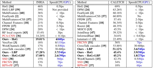
Method INRIA Speed(CPU/GPU)
HoG [16] 46% 0.5fps
HoG-LBP [59] 39% Not provided
MultiFeatures [60] 36% < 1fps FeatSynth [2] 31% < 1fps MultiFeatures+CSS [57] 25% No Channel Features [18] 21% 0.5fps FPDW [17] 21% 2-5fps DPM [24] 20% < 1fps RF local experts [43] 15.4% 3fps PCA-CNN[36] 14.24% < 0.1fps Ours - HoG 19.01% 4/60fps VeryFast [3] 18% 8/135fps WordChannels [15] 17% 0.5/8fps crossTalk cascades [19] 17% 30-60fps Ours - LBP 17.28% 3.7/54fps Ours - HoG+LBP 17.08% 2.6/39fps SSD[38] 15% 56fps FRCNN[51] 13% 7fps RPN+PF[37] 7% 6fps
Method CALETCH Speed(CPU/GPU)
HoG [16] 69% 0.5fps DPM [24] 63.26% < 1fps FeatSynth [2] 60.16% < 1fps MultiFeatures+CSS [57] 60.89% No FPDW [17] 57.4% 2-5fps Channel Features [18] 56.34% 0.5fps Roerei [4] 48.35% 1 fps MOCO [13] 45.5% < 1fps JointDeep [47] 39.32% < 1fps InformedHaar [66] 34.6% < 0.63fps katamari-v1 [5] 22.49% < 1fps FRCNN[51] 56% 7fps CrossTalk cascades [19] 53.88% 30-60fps Ours - LBP 51.12% 3.6/54fps Ours - HoG 45.4% 3.9/58fps Ours - HoG+LBP 45.2% 1.8/27fps WordChannels [15] 42.3% 0.5/8fps SSD[38] 34% 56fps RPN+PF[37] 10% 6fps TABLE VI
COMPARISON WITH THE STATE-OF-THE-ART. NEAR REAL-TIME METHODS ARE SEPARATED FROM OTHERS. OursIS IN BOLD. DEEP LEARNING TECHNIQUES ARE IN RED. COMPUTATION TIMES ARE CALCULATED ACCORDING TO640×480RESOLUTION FRAMES. THE USED METRIC IS THE
LOG-AVERAGE MISS RATE(THE LOWER THE BETTER).
Soft cascade type Feature INRIA Caltech No soft-cascade HoG 20.31% / 2.1fps 46.25% / 1.9fps
soft-cascade HoG 32.21% / 18.1fps 58.26% / 17.8fps block soft-cascade HoG 27.86% / 9.9fps 53.97% / 10.1fps reverse engineering HoG 20.32% / 4 fps 46.23%/ 3.9fps
No soft-cascade LBP 18.42% / 1.9fps 51.36% / 1.7fps soft-cascade LBP 30.87% / 17.8fps 61.32% / 17.1fps block soft-cascade LBP 28.33% / 9.8fps 55.45% / 9.5fps reverse engineering LBP 18.41%/ 3.7fps 51.33% / 3.6fps
TABLE VII
LAMRPERFORMANCE ANDCPUSPEED IN FRAME-PER-SECOND OF DIFFERENT SOFT-CASCADE STRATEGIES. SEE TEXT FOR THE DESCRIPTION
OF THE METHODS. BEST RESULTS IN BOLD.
each step (4) perform poorly when used with these classifiers settings. The best performing thresholding technique uses a constant threshold (1). This technique leads to an average deletion of respectively 80% and 35% of the data during the first 2 steps of the cascade, and 5-10% during the remaining stages. Hence, we assume that the thresholding technique (3) and (4) might also be dependent to classifier sets displaying a rather regular deletion behaviour across the cascade steps.
Finally, all the tested techniques, are, on average performing 4.48% worse than the optimal. This elects threshold estimation as a potentially rewarding research direction.
lesson learned: Counter-intuitively, the variability between the threshold values is not much caused by the data, but mostly by the features. None of existing approaches are close to the optimal and there is still space for improvement in that particular direction.
J. Non maximum suppression
Table IX covers our evaluation the 3 existing non-maximum suppression algorithms previously described in section III-G. The best results for both HoG and LBP features are always obtained by the threshold non-maximum suppression with an average 2% boost compared to the common greedy non-maximum suppression.
lesson learned: Surprisingly, the choice of the non max-imum suppression algorithm significantly impacts the
over-Thresholding strategy Feature INRIA Caltech Optimal HoG 17.89% 42.67% Constant HoG 20.23% 46.25% Increasing HoG 21.44% 47.25% Recall HoG 25.01% 50.88% Regular HoG 27.11% 51.84% Optimal LBP 15.44% 42.45% Constant LBP 18.63% 51.26% Increasing LBP 19.96% 51.78% Recall LBP 22.34% 54.88% Regular LBP 22.36% 62.53% TABLE VIII
THRESHOLD ESTIMATION TECHNIQUES EVALUATION ONINRIAAND
CALTECH BENCHMARKS. SEE TEXT FOR THE DESCRIPTION OF THE METHODS. BEST RESULTS IN BOLD.
NMS type Feature INRIA Caltech Greedy-NMS HoG 22.91% 49.62% t-NMS HoG 20.23% 46.25% s-NMS HoG 21.47% 46.98% Greedy-NMS LBP 20.21% 52.32% t-NMS LBP 18.63% 51.26% s-NMS LBP 19.87% 52.65% TABLE IX
NON-MAXIMUM SUPPRESSION ALGORITHM EVALUATION ONINRIAAND
CALTECH BENCHMARKS. BEST RESULTS IN BOLD.
all detector performance. The over-employed greedy non-maximum suppression, that underperforms in every case, shouldn’t be blindly chosen.
K. Comparison with the state-of-the-art
Table VI shows our method’s ranking compared to the state-of-the-art, in terms of performance and speed. Table I param-eters and random forest were employed for this experiment.
T =0.58 is used for these runs. This work compares favorably
to the state-of-the-art. We used using Adaboost classifiers and soft coding reverse engineering for this experiment.While not being the best detector on the market, with respectively 17% and 46% log-average miss rate on the INRIA and Caltech datasets, our approach still provides a very competitive performance/speed ratio. For instance, it scores better than
the famous DPM [24] and similarly to the integral channel features [17] while running 7 times faster. VeryFast [3] and the crosstalk cascades provide a viable alternative in terms of speed while displaying lower performance. LBP is the best descriptor on the INRIA dataset, while HoGs show the best performance on Caltech. We assume that the numerous little pedestrians on the latter impact the texture descriptor more strongly than the gradients. The HoG and LBP fusion yields little improvement. Packed crowds, teensy pedestrians and awkward poses remain the main failure cases. Finally, Deep learning technique [36], [51] perform worse and are slower, [37] performs much better but is slower, while [38] is slightly more efficient and faster. It is worth stating that careful machine learning choices and parametrisation can bring standard features close to state-of-the-art deep learning performance. The end-to-end system is trained in 4-14hours on one core for 10-200K data and processes 3-4 fps on an Intel Xeon 2.1GHz CPU, calculated over frames of 640×480 pixels in size. Further speed up is possible when using a GPU, leading our detector to perform in real-time. This makes this detector one of the best performing real-time pedestrian detector to date.
V. CONCLUSION
This paper studied through extensive experimentation under-explored mechanisms at various stages of a pedestrian clas-sifier training, with an emphasis on data selection, dataset generation at the initial stage and during the classifier cascade. Our study highlighted data selection and non-maximum sup-pression as underexploited components for high performance, and soft-cascade thresholding assessment as potential research direction. We also disproved a few empirically received ideas, namely the predominance of the random forest classifier (with high performing detectors) or the use of the DBSCAN algorithm for data cleaning.
Besides extra experiments in domains such as active learning or part-based models, the application of the optimized
Fair-Train pipeline to deep learning is an obvious possible next
step for this work.
VI. ACKNOWLEDGMENT
To appear in camera ready version. REFERENCES
[1] T. Ahonen, A. Hadid, and M. Pietikinen. Face description with local bi-nary patterns: Application to face recognition. PAMI, 28(12):20372041, 2006.
[2] A. Bar-Hillel, D. Levi, E. Krupka, and C. Goldberg. Part-based feature synthesis for human detection. ECCV, 2010.
[3] R. Benenson, M. Mathias, R. Timofte, and L. V. Gool. Pedestrian detection at 100 frames per second. CVPR, 2013.
[4] R. Benenson, M. Mathias, T. Tuytelaars, and L. V. Gool. Seeking the strongest rigid detector. CVPR, 2013.
[5] R. Benenson, M. Omran, J. Hosang, and B. Schiele. Ten years of pedestrian detection, what have we learned? ECCV, CVRSUAD workshop, 2014.
[6] Y. Bengio, J. Louradour, R. Collobert, and J. Weston. Curriculum learning. ICML, 2009.
[7] B. Berkin, B. K. Horn, and I. Masaki. Fast human detection with cascaded ensembles on the gpu. IEEE Intelligent Vehicles Symposium, 2010.
[8] L. Bourdev and J. Brandt. Robust object detection via soft cascade.
CVPR, 20105.
[9] L. Breiman. Random forests. Machine Learning, 2001.
[10] M. D. Buil. Non-maximum suppression. technical report ICG-TR-xxx, 2011.
[11] X. Chang, Z. Ma, M. Lin, Y. Yang, and A. Hauptmann. Feature interaction augmented sparse learning for fast kinect motion detection.
IEEE Transactions on Image Processing, 26(8):3911–3920, 2017.
[12] X. Chang, Y. Yu, Y. Yang, and E. P. Xing. Semantic pooling for complex event analysis in untrimmed videos. PAMI, 39(8):1617–1632, 2017. [13] G. Chen, Y. Ding, J. Xiao, and T. X. Han. Detection evolution with
multi-order contextual co-occurrence. CVPR, 2013.
[14] E. Corvee and F. Bremond. Haar like and lbp based features for face, head and people detection in video sequences. ICVS, 2011.
[15] A. D. Costea and S. Nedevschi. Word channel based multiscale pedestrian detection without image resizing and using only one classifier.
CVPR, 2014.
[16] N. Dalal and B. Triggs. Histograms of oriented gradients for human detection. CVPR, 2005.
[17] P. Dollar, S. Belongie, and P. Perona. The fastest pedestrian detector in the west. BMVC, 2010.
[18] P. Dollar, Z. Tu, P. Perona, and S. Belongie. Integral channel features.
BMVC, 2009.
[19] P. Dollr, R. Appel, and W. Kienzle. Crosstalk cascades for frame-rate pedestrian detection. ECCV, 2012.
[20] P. Dollr, C. Wojek, B. Schiele, and P. Perona. Pedestrian detection: A benchmark. CVPR, 2009.
[21] P. G. Doyle and J. L. Snell. Random walks and electric networks. MAA, 1984.
[22] C. Elkan. The foundations of cost-sensitive learning. Intl Joint Conf.
Artificial Intelligence, 2001.
[23] M. Ester, H.-P. Kriegel, J. S. X. Xu, E. Simoudis, J. Han, and U. M. Fayyad. A density-based algorithm for discovering clusters in large spatial databases with noise. KDD-96, page 226231, 1996.
[24] P. Felzenszwalb, R. Girshick, D. McAllester, and D. Ramanan. Ob-ject detection with discriminatively trained part-based models. PAMI, 32(9):1627–1645, 2009.
[25] P. F. Felzenszwalb, R. B. Girshick, and D. McAllester. Cascade object detection with deformable part models. CVPR, 2010.
[26] J. Ferryman and A. Shahrokni. An overview of the pets2009 challenge.
PETS, 2009.
[27] J. Gall and V. Lempitsky. Class-specific hough forests for object detection. CVPR, 2009.
[28] C. Galleguillos and S. Belongie. Context based object categorization: A critical survey. CVIU, 114:712–722, 2010.
[29] H. Han, W. Wang, and B. Mao. Borderline-smote: A new over-sampling method in imbalanced data sets learning. Intl Conf. Intelligent
Computing, 2005.
[30] H. He, Y. Bai, E. Garcia, and S. Li. Adasyn: Adaptive synthetic sampling approach for imbalanced learning. Intl J. Conf. Neural Networks, 2008. [31] H. He and E. A. Garcia. Learning from imbalanced data. IEEE transactions on Knowledge and data engineering, 21(9):1263–1284,
2009.
[32] A. Hoiem and M. Efros. Putting objects in perspective. IJVC, 2008. [33] S. Hwang, T.-H. Oh, and I. S. Kweon. A two phase approach for
pedestrian detection. ACCV, 2014.
[34] N. Japkowicz. Learning from imbalanced data sets: a comparison of various strategies. AAAI Workshop on Learning from Imbalanced Data
Sets, 2000.
[35] T. Jo and N. Japkowicz. Class imbalances versus small disjuncts. ACM
SIGKDD Explorations Newsletter, 6(1):40–49, 2004.
[36] W. Ke, Y. Zhang, P. Wei, Q. Ye, and J. Jiao. Pedestrian detection via pca filters based convolutional channel features. ICASSP, 2015. [37] Z. Liliang, L. Liang, L. Xiaodan, and H. Kaiming. Is faster r-cnn doing
well for pedestrian detection? ECCV, pages 443–457, 2016.
[38] W. Liu, D. Anguelov, D. Erhan, C. Szegedy, S. Reed, C.-Y. Fu, and A. C. Berg. Ssd: Single shot multibox detector. ECCV, 2016. [39] W. Liu, X. Chang, L. Chen, and Y. Yang. Early active learning with
pairwise constraint for person re-identification. ECML, 2017. [40] W. Liu, C. Gao, X. Chang, and Q. Wu. Unified discriminating
feature analysis for visual category recognition. Journal of Visual Communication and Image Representation, 40:772–778, 2016.
[41] M. Luo, X. Chang, L. Nie, Y. Yang, A. Hauptmann, and Q. Zheng. An adaptive semi-supervised feature analysis for video semantic recognition.
IEEE Transactions on Cybernetics, 48(2):648–660, 2018.
[42] Z. Ma, X. Chang, Z. Xu, N. Sebe, and A. G. Hauptmann. Joint attributes and event analysis for multimedia event detection. IEEE Trans. Neural
Netw. Learning Syst., 29(7):2921–2930, 20018.
[43] J. Marin, D. Vazquez, A. M. Lopez, J. Amores, and B. Leibe. Random forests of local experts for pedestrian detection. ICCV, 2013. [44] W. Nam, P. Dollar, and J. H. Han. Local decorrelation for improved
pedestrian detection. NIPS, 2014.
rotation invariant texture classification with local binary patterns. PAMI, 24(7):971–987, 2002.
[46] T. Ojala, M. Pietikinen, and D. Harwood. A comparative study of texture measures with classification based on feature distributions. Pattern Recognition, 29:51–59, 1996.
[47] W. Ouyang and X. Wang. Joint deep learning for pedestrian detection.
ICCV, 2013.
[48] W. Ouyang and X. Wang. Single-pedestrian detection aided by multi-pedestrian detection. CVPR, 2013.
[49] D. P, C. Wojek, B. Schiele, and P. Perona. Pedestrian detection: An evaluation of the state of the art. PAMI, 34(4):743–761, 2012. [50] D. Park, D. Ramanan, and C. Fowlkes. Multiresolution models for object
detection. ECCV, 2010.
[51] S. Ren, K. Hen, R. Girshick, and J. Sun. Faster r-cnn: Towards real-time object detection with region proposal networks. NIPS, 2015.
[52] M. Souded and F. Bremond. Optimized cascade of classifiers for people detection using covariance features. VISAPP, 2013.
[53] K. Ting. An instance-weighting method to induce cost-sensitive trees,.
IEEE Trans. Knowledge and Data Eng., 14(3):659–665, 2002.
[54] I. Tomek. Two modifications of cnn. IEEE Trans. System, Man, Cybernetics, 6(11):769–772, 1976.
[55] R. Trichet and F. Bremond. Dataset optimisation for real-time pedestrian detection. IEEE access, 6:7719 – 7727, 2018.
[56] Viola and M. Jones. Rapid object detection using a boosted cascade of simple features. CVPR, 2001.
[57] S. Walk, N. Majer, K. Schindler, and B. Schiele. New features and insights for pedestrian detection. CVPR, 2010.
[58] B. Wang and N. Japkowicz. Imbalanced data set learning with synthetic samples. IRIS Machine Learning Workshop, 2004.
[59] X. Wang, T. X. Han, and S. Yan. An hog-lbp human detector with partial occlusion handling. ICCV, 2009.
[60] C. Wojek and B. Schiele. A performance evaluation of single and multi-feature people detection. DAGM Symposium Pattern Recognition, pages 82–91, 2008.
[61] B. Wu and R. Nevatia. Cluster boosted tree classifier for multi-view, multi-pose object detection. ICCV, 2007.
[62] Y. Y. X. Chang, L. Chen. Semi-supervised bayesian attribute learning for person re-identification. AAAI, 2018.
[63] R. S. Y. Freund. A decision-theoric generalization of online learning and an application to boosting. Journal of Computer and System Sciences, 55(1):119139, 1997.
[64] J. Yan. Robust multi-resolution pedestrian detection in traffic scenes.
CVPR, 2013.
[65] R. Yan, Y. Liu, R. Jin, and A. G. Hauptmann. On predicting rare classes with svm ensemble in scene classification. ICASSP, 2003.
[66] S. Zhang, C. Bauckhage, and A. B. Cremers. Informed haar-like features improve pedestrian detection. CVPR, 2014.
[67] S. Zhang, R. Benenson, M. Omran, J. Hosang, and B. Schiele. How far are we from solving pedestrian detection. CVPR, 2016.
[68] Z. Zhiqiang, L. Zhihui, C. De, Z. Huaxzhang, Z. Kun, and Y. Yi. Two-stream multi-rate recurrent neural network for video-based pedestrian re-identification. IEEE Transactions on Industrial Informatics, 14(7):3179– 3186, 2017.
[69] Q. Zhu, S. Avidan, M. Yeh, and K. Cheng. Fast human detection using a cascade of histograms of oriented gradients. CVPR, 2006.