HAL Id: hal-02884947
https://hal.archives-ouvertes.fr/hal-02884947
Submitted on 30 Jun 2020
HAL is a multi-disciplinary open access
archive for the deposit and dissemination of
sci-entific research documents, whether they are
pub-lished or not. The documents may come from
L’archive ouverte pluridisciplinaire HAL, est
destinée au dépôt et à la diffusion de documents
scientifiques de niveau recherche, publiés ou non,
émanant des établissements d’enseignement et de
Shifted-Chebyshev-polynomial-based numerical
algorithm for fractional order polymer visco-elastic
rotating beam
Lei Wang, Yi-Ming Chen
To cite this version:
Lei Wang, Yi-Ming Chen. Shifted-Chebyshev-polynomial-based numerical algorithm for fractional
or-der polymer visco-elastic rotating beam. Chaos, Solitons and Fractals, Elsevier, 2020, 132, pp.109585.
�10.1016/j.chaos.2019.109585�. �hal-02884947�
Shifted-Chebyshev-polynomial-based numerical
algorithm for fractional order polymer visco-elastic
rotating beam
Lei Wanga, Yi-Ming Chena,b,c,∗
aSchool of Sciences, Yanshan University, Qinhuangdao, Hebei, P.R.China, 066004.
bLE STUDIUM RESEARCH PROFESSOR, Loire Valley Institute for Advanced Studies,
Orl´eans, France
cINSA - Institut National des sciences appliqu´ees - 88, Boulevard Lahitolle, Blois Cedex,
France
Abstract
In this paper, an effective numerical algorithm is proposed for the first time to solve the fractional visco-elastic rotating beam in the time domain. On the basis of fractional derivative Kelvin-Voigt and fractional derivative element con-stitutive models, the two governing equations of fractional visco-elastic rotating beams are established. According to the approximation technique of shifted Chebyshev polynomials, the integer and fractional differential operator matri-ces of polynomials are derived. By means of the collocation method and matrix technique, the operator matrices of governing equations can be transformed into the algebraic equations. In addition, the convergence analysis is performed. In particular, unlike the existing results, we can get the displacement and the stress numerical solution of the governing equation directly in the time domain. Finally, the sensitivity of the algorithm is verified by numerical examples.
Keywords: Fractional visco-elastic rotating beam, Fractional governing
equation, Shifted Chebyshev polynomials, Approximation technique, Operator matrix, Numerical solution
1. Introduction
Fractional calculus and fractional differential equations have been widely used in physics, engineering, economics and other research fields [1–5], since fractional derivative has better memory [6] than integer order one, especially in the application of visco-elastic polymer materials. The fractional order consti-tutive model [7–12] can describe material properties more accurately with fewer parameters, so it is considered to be a good mathematical model to describe the
∗Corresponding author.
dynamic mechanical behavior of visco-elastic materials. There are also many researches on fractional order visco-elastic beams [13–18].
The complexity of the fractional derivative determines that the numerical solution of the beam governing equation became more difficult to deal with. Scholars have used Laplace or Fourier transform to transform the time domain problem into a frequency domain problem to study the fractional order govern-ing equation in the frequency domain. For example, Lewandowski et al. [14, 19] used fractional four-parameter model and fractional Zener model to describe visco-elastic materials. The virtual work principle and Laplace transform have been used to derive the motion equations of the considered system in the fre-quency domain, and then the dynamic characteristics of the visco-elastic beam have been studied. Kiasat et al. [20] used the Fourier transform to calculate the unknown coefficient of the dynamic response function to research the free vibration of isotropic visco-elastic beams and plates on visco-elastic media. The process of solving the fractional visco-elastic governing equations in the variable domain was complicated. This has led scholars to solve the analysis in the time domain.
Methods for solving fractional visco-elastic beams in the time domain include the finite element method [21, 22], multi-scale method [23], Galerkin method [24] and the variational iteration method [25] which have been found in the literature. But so far, the numerical solutions of the displacement and the stress of fractional visco-elastic rotating beams in time domain has not been studied.
As an important tool for the in-depth research and development of math-ematics, function approximation theory has been successfully applied in the fields of control science and engineering, mechanical engineering, system sci-ence and so on [26–30]. It is well known that the study of numerical solutions of fractional visco-elastic beams can be attributed to the problem of solving fractional differential equations. The solutions of fractional differential equa-tions mainly include analytical methods, polynomial approximation methods and other methods. Due to the complex form of fractional derivative, the so-lution of the fractional order differential equation is intractable to obtain. The analytical method has tedious numerical calculation and limited to solving some simple problems. Compared with the former, the polynomial approximation method of fractional differential equations is particularly significant because of its fast speed, high efficiency and high precision. Polynomial approxima-tion methods include Legendre polynomial method [31, 32], Chebyshev wavelet method [33, 34], Bernoulli wavelet method [35], Bernstein polynomial method [36, 37] and shifted Chebyshev polynomials (SCPs) method [38]. The SCPs method can be used to approximate the unknown function on the extended in-terval, which makes it easier to solve the fractional differential equations with different physical mechanisms governing and historical background [39–42].
Rotating beams has been widely used in helicopter rotors, wind turbine blades, propellers and various rotating mechanical structures. The study of the vibration characteristics of the rotating beams [43–46] has been an important basis for the design of the rotating beam machinery. Based on this, in this paper,
we use the fractional derivative element (FDE) and the fractional derivative Kelvin-Voigt (FDKV) constitutive models. Polymers Poly(ether ether ketone) (PEEK) rotating beam and High-density polyethylene (HDPE) [47] rotating beam are studied by SCPs method. The SCPs algorithm is solved directly in the time domain, the process is simple, and the numerical solutions of the displacement and the stress of the fractional visco-elastic rotating beam can be obtained.
This paper is structured as follows, in Section 2, some preliminaries including the basic definition of fractional differential operators, the fractional visco-elastic constitutive models and the properties of SCPs are described. In Section 3, the SCPs solving algorithm is described. In Section 4, FDE model and FDKV model are used to establish two governing equations of visco-elastic rotating beam. The convergence analysis is performed in Section 5. In Section 6, the numerical results of the displacement and the stress of the visco-elastic rotating beams are obtained and discussed to show the advantages of the proposed approach. The research work in this paper is concluded in Section 7.
2. Preliminaries and notations
Some basic definitions and properties of the fractional order calculus are provided in this section.
2.1. The basic definition of fractional differential operator
Definition 1. [48] The Caputo definition of fractional differential operator
(cDαf ) of order α is given by�
(cDαf )(t) = 1 Γ(m−α) ∫t 0 f(m)(τ ) (t−τ)α−m+1dτ , α > 0, m− 1 ≤ α < m, dmf (t) dtm , α = m. (1)
for the Caputo derivative, we have�
cDαtχ= {
0, for χ∈ N0 and χ < α,
Γ(χ+1) Γ(χ+1−α)t
χ−α, for χ∈ N0 and χ≥ α or χ /∈ N0 and χ > α. (2)
It has following two basic properities for m− 1 ≤ α < m and f ∈ L1[a, b]:
(cDαcIαf )(t) = f (t) (3) and (cIαcDαf )(t) = f (t)−∑m−1 k=0 f (k)(0+)(t− a) k k! , t > 0 (4)
2.2. Properties of the SCPs
SCPs are considered as useful tools to solve the fractional equation in the physical problems. The well-known Chebyshev polynomials satisfy the following term recurrence relation:
Ti+1(t) = 2tTi(t)− Ti−1(t), i = 1, 2, ... (5) where T0(t) = 1, T1(t) = t. t is defined on the interval [−1, 1] and i = 1, 2,· · ·.
On the interval [0, L], where L is a non-negative real number, the SCPs are defined by the change of variable t = 2x
L − 1. Let the SCPs Ti( 2x
L − 1) denote by Gi(x), which can be obtained as follows:
Gi+1(x) = 2( 2x
L − 1)Gi(x)− Gi−1(x), i = 1, 2, ... (6)
where G0(x) = 1, G1(x) = 2x
L − 1. The analytic form of Gi(x) of i-degree is given by: Gi(x) = i i ∑ k=0 (−1)i−k(i + k− 1)!2 2k (i− k)!(2k)!Lkx k, i = 1, 2,... (7)
where Gi(0) = (−1)i and Gi(L) = 1. The orthogonally condition is ∫ L 0 Gj(x)Gk(x)ωL(x)dx = hk, (8) where ωL(x) = √Lx1−x2 and hk = { b k 2π, k = j, 0, k̸= j, b0= 2, bk = 1, k≥ 1. The operational matrix is defined by:
Φn(x) = [G0(x), G1(x),· · · , Gn(x)] T
(9) The following equation can be obtained:
Φn(x) = AnZn(x) (10)
where Zn(x) = [
1, x, x2,· · · , xn]T, and An is the SCPs coefficient matrix given as follows: An = P0,0 0 · · · 0 P1,0 P1,1 · · · 0 .. . ... . .. ... Pn,0 Pn,1 · · · Pn,n , (11) where P0,0= 1, Pi,j= 2(L2Pi−1,j−1− Pi−1,j)− Pi−2,j, Pi,j= 0, for i < j or i < 0 or j < 0.
Obviously, An is full rank and reversible.
2.3. Visco-elastic constitutive and fractional derivative models
The general form of a one-dimensional generalized fractional constitutive equation describing the stress-strain relationship of a visco-elastic material is:
n ∑ κ=0 µκ dpκσ(t) dtpκ = n ∑ κ=0 ηκ dqκε(t) dtqκ (12)
where dκ/dtκ uses the Caputo type fractional differential definition, σ is the stress, ε is the strain, µκ, ηκ are the material constants. κ is a positive inte-ger. And pκ, qκ are real numbers corresponding to fractional order of the time derivative.
When pκ, qκ= 0, the constitutive equation becomes ideal elastic behaviour law or Hooke’s law. When pκ = 0, qκ = 1, the constitutive equation becomes ideal viscous behaviour law or Newton’s law. When 0 < qκ< 1, the constitutive equation could be used to describe the physical behaviour of a visco-elastic material. In the current visco-elastic constitutive fractional derivative models, the first order derivatives d/dt are replaced by the fractional derivatives dqκ/dtqκ
with 0 < qκ< 1.
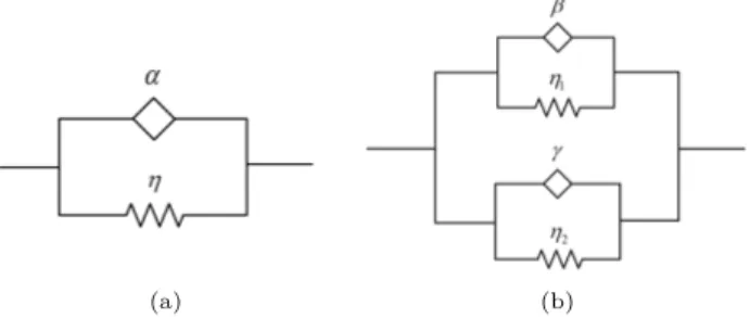
(a) (b)
Fig. 1. Schematic representation of visco-elastic model: (a) the FDE model; (b) the FDKV
model.
The simplest fractional model of visco-elastic media is the FDE model [47] as shown in Fig. 1(a), which has the following form of stress-strain relationship�
σ(t) = ηd αε(t)
dtα (13)
By replacing the elastic and viscous elements of the classical linear viscoelas-tic model with fractional elements, two fractional elements arranged in parallel can obtained as shown in Fig. 1(b), which is the FDKV model [47]. And its constitutive equation as follows:
σ(t) = η1
dβε(t) dtβ + η2
dγε(t)
dtγ (14)
3. Numerical algorithm 3.1. Approximation of function
For arbitrary continuous function ω(x, t) ∈ L2([0, L] × [0, T ]), it can be expanded as the following formula:
ω(x, t) = ∞ ∑ i=0 ∞ ∑ j=0 ωijGi(x)Gj(t) (15) where ωij =h1 ihj ∫L 0 ∫T 0 ω(x, t)Gi(x)Gj(t)ωL(x)ωT(t)dtdx, i, j = 0, 1, 2,· · ·. If we consider truncated series in Eq. (15), then it can rewritten as:
ω(x, t)≈ n ∑ i=0 n ∑ j=0 ωijGi(x)Gj(t) = ΦTn(x)U Φn(t) (16) where Φn(x) = [G0(x), G1(x),· · · , Gn(x)] T , Φn(t) = [G0(t), G1(t),· · · , Gn(t)] T , U ={uij} n,n i,j=0.
3.2. SCPs differential operator matrix
3.2.1. First order differential operator matrix of SCPs
Definition 2. If there is matrix Px(1), satisfying dxdΦn(x) = P
(1)
x Φn(x), then Px(1) is called the first order differential operator matrix of SCPs.
By calculating the first order derivative of Φn(x), dxdΦn(x) can expressed as: d dxΦn(x) = (AXZn(x)) ′= A XZn′(x) = AX 1′ x′ .. . (xn)′ = AX 0 1 .. . nxn−1 = AXV(n+1)×nZn∗(x) (17) and V(n+1)×n= 0 0 · · · 0 1 0 · · · 0 0 2 · · · 0 .. . ... . .. 0 0 0 · · · n , Zn∗(x) = 1 x .. . xn−2 xn−1 (18)
By using Eq. (10), Zn∗(x) is obtained as:
where BX∗ = [
A−1X, [1], A−1X, [2], · · · , A−1X, [n]
]T . According to Eq. (16), Eq. (19) can rewritten as:
d
dxΦn(x) = AXV(n+1)×nB ∗
XΦn(x) (20)
where Px(1)= AXV(n+1)×nBX∗ is a first order differential operator matrix of the SCPs. Substituting Eq. (11), Eq. (17) and matrix BX∗ into P
(1) x : Px(1)= [λ0, λ1, · · · , λi, · · · , λn]T, i = 0, 1, · · · , n (21) where λi= i ∑ j=1 jPijA−1x, [j].
Now, using Eq. (16) and Eq. (20), we get:
∂ω(x, t) ∂x ≈ ∂(ΦTn(x)U Φn(t)) ∂x = ΦTn(x)(Px(1))TU Φn(t) = ΦTn(x)(AXV(n+1)×nBX∗) TU Φ n(t) (22)
Furthermore, the higher-order differential operator matrices derived from SCPs by mathematical induction have the following form:
dn dxnΦn(x) = ( Px(1) )n Φn(x) (23)
3.2.2. Fractional order differential operator matrix of the SCPs
Definition 3. If there is matrix Pβ
t(t), satisfyingcD β
tΦn(t) = Ptβ(t)Φn(t), then Ptβ(t) is called fractional order differential operator matrix of SCPs.
By taking the fractional derivative of Φn(t), we obtain:
cDβ tω(x, t)≈cD β t ( ΦTn(x)U Φn(t) ) = ΦT n(x)UcD β tΦn(t) = ΦT n(x)U [ 0, · · · , Γ (β + 1) Γ (β + 1− β)t β−β, · · · , Γ (i + 1) Γ (i + 1− β)t i−β, · · ·]T = ΦT n(x)U ATV(n+1)β ×(n+1)A−1T Φn(t) (24)
where i = β, β + 1, · · · , n, Pβ t(t) = ATV(n+1)β ×(n+1)A−1T , and V(n+1)β ×(n+1)= 0 · · · 0 · · · 0 · · · 0 . .. . .. ... ... ... ... ... 0 · · · Γ(β+1)tΓ(β+1−β)−β · · · 0 · · · 0 .. . ... ... . .. ... ... ... 0 · · · 0 · · · Γ(i+1)tΓ(i+1−β)−β · · · 0 .. . ... ... ... ... . .. ... 0 · · · 0 · · · 0 · · · Γ(m+1)tΓ(m+1−β)−β (25)
The fractional order differential operator matrix Ptβ(t) is
Ptβ(t) = 0 · · · 0 · · · 0 · · · 0 .. . ... ... ... ... ... ... 0 · · · 0 · · · 0 · · · 0 Sβ(β, 0) · · · Sβ(β, β) · · · 0 · · · 0 .. . ... ... . .. ... ... ...
Sβ(i, 0) · · · Sβ(i, β) · · · Sβ(i, i) · · · 0
.. . ... ... ... ... . .. ... Sβ(n, 0) · · · Sβ(n, β) · · · Sβ(n, i) · · · Sβ(n, n) (26)
4. Establishment and solution of government equations for visco-elastic rotating beam
4.1. Beam governing equation under the FDKV model
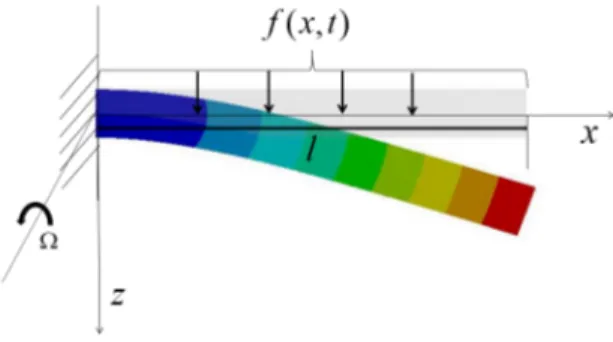
A visco-elastic rotating beam is considered in this study. A distributed load is applied on the vertical direction of the beam. The beam is made of a visco-elastic material. The bending deformation occurs on the beam in the vertical direction, as shown in Fig. 2, in which ω(x, t) is the beam deflection, f (x, t) is the distributed load, Ω is the speed and l is the length of the beam.
For visco-elastic beams, the stress and strain satisfy the two-dimensional FDKV model can be expressed as:
σ(x, t) = η1cD β
tε(x, t) + η2cD γ
tε(x, t) (27)
where ε(x, t) is the transverse strain, η1, η2, β, γ are parameters of visco-elastic material,cDβ
t, cDγ
t use the Caputo type fractional differential definition. The relation between the strain and the displacement can be expressed as:
ε(x, t) = z∂
2ω(x, t)
∂x2 (28)
Fig. 2. The bending deformation of the visco-elastic rotating beam under distributed load.
The bending moment M (x, t) of the beam is written as:
M (x, t) =
∫ A
zσ(x, t)dz (29)
where σ(x, t) is the normal stress on the cross-section.
Using Eq. (27), the beam bending moment M (x, t) is equal to:
M (x, t) = η1IcDβt ∂2ω(x, t) ∂x2 + η2I cDγ t ∂2ω(x, t) ∂x2 (30)
where I is the moment of inertia of the section given by∫Az2dA.
The potential energy of the rotating beam is
U =1 2 ∫ L 0 M (x, t)∂ 2ω(x, t) ∂x2 dx + 1 2 ∫ L 0 Tx ∂2ω(x, t) ∂x2 dx (31)
Rotating centrifugal force Tx can be expressed as:
Tx= ρAΩ2x (32) Kinetic energy is T =1 2 ∫ L 0 ρA∂ 2ω(x, t) ∂t2 dx (33)
The beam is subjected to a load of f (x, t), according to the Hamiltonian principle, we obtain that
δ ∫ t2 t1 (T− U)dt + ∫ t2 t1 δW dt = 0 (34)
The governing equation of the visco-elastic rotating beam under the FDKV constitutive model is obtained:
ρA∂ 2ω(x, t) ∂t2 +η1I C Dtβ ∂4ω(x, t) ∂x4 +η2I C Dtγ ∂4ω(x, t) ∂x4 −ρAΩ 2 x∂ 2ω(x, t) ∂x2 = f (x, t) (35)
4.2. Beam governing equation under the FDE model
The stress and strain satisfy the FDE constitutive model is proposed:
σ(x, t) = ηcDtαε(x, t) (36) According to Eq. (36), the beam bending moment M (x, t) can be rewritten as:
M (x, t) = ηIcDαt∂
2ω(x, t)
∂x2 (37)
where I is the moment of inertia of the section given by∫Az2dA.
The governing equation of the visco-elastic rotating beam under the FDKV constitutive model is obtained as follows:
ρA∂ 2ω(x, t) ∂t2 + ηI cDα t ∂4ω(x, t) ∂x4 − ρAΩ 2x∂ 2ω(x, t) ∂x2 = f (x, t) (38)
4.3. The solution of governing equation based on SCPs
Based on integer order differential operator matrix of SCPs in the Section 3.2.1, the following equations can be obtained:
∂2ω(x, t) ∂x2 ≈ ∂2(ΦT n(x)U Φn(t)) ∂x2 = ΦTn(x)((Px(1))T)2U Φn(t) = ΦTn(x)((AXV(n+1)×nBX∗) T)2U Φ n(t) (39) ∂4ω(x, t) ∂x4 ≈ ∂4(ΦT n(x)U Φn(t)) ∂x4 = ΦTn(x)((Px(1))T)4U Φn(t) = ΦTn(x)((AXV(n+1)×nBX∗) T)4U Φ n(t) (40) ∂2ω(x, t) ∂t2 ≈ ∂2(ΦT n(x)U Φn(t)) ∂t2 = ΦTn(x)U (Pt(1))2Φn(t) = ΦTn(x)U (ATV(n+1)×nBT∗) 2Φ n(t) (41)
3.2.2, the following equations can be obtained: cDβ t ∂4ω(x, t) ∂x4 ≈ cDβ tΦTn(x) ( (AXV(n+1)×nBX∗) T)4 U Φn(t) = ΦTn(x) ( (AXV(n+1)×nBX∗) T)4 UcDβtΦn(t) = ΦTn(x) ( (AXV(n+1)×nBX∗) T)4 U ATPtβ(t)A−1T Φn(t) (42) Similarly, cDγ t ∂4ω(x, t) ∂x4 ≈ cDγ tΦ T n(x) ( (AXV(n+1)×nBX∗) T)4 U Φn(t) = ΦTn(x) ( (AXV(n+1)×nBX∗) T)4 UcDγtΦn(t) = ΦTn(x) ( (AXV(n+1)×nBX∗) T)4 U ATPtγ(t)A−1T Φn(t) (43) where Pγ
t(t) is obtained by replacing β with γ in Eq. (26).
The gverning equation Eq. (35) can be rewritten into the operator matrix form as follows: ρAΦTn(x)U ( Pt(1) )2 Φn(t) + η1IΦTn(x) ( (Px(1)) T)4 U Ptβ(t)Φn(t) +η2IΦTn(x) ( (Px(1)) T)4 U Ptγ(t)Φn(t)− ρAΩ2xΦTn(x) ( (Px(1)) T)2 U Φn(t) = f (x, t) (44)
Specifically, Eq. (44) can be written as:
ρAΦTn(x)U ( ATV(n+1)×nB∗T )2 Φn(t) + η1IΦTn(x) ( (AXV(n+1)×nBX∗) T)4 U AT× V(n+1)β ×(n+1)A−1T Φn(t) + η2IΦTn(x) ( (AXV(n+1)×nBX∗) T)4U A T× V(n+1)γ ×(n+1)A−1T Φn(t)− ρAΩ2x ( (AXV(n+1)×nB∗X) T)2 U Φn(t) = f (x, t) (45)
Similarly, the governing equation Eq. (38) can be rewritten into the operator matrix form as follows:
ρAΦTn(x)U ( Pt(1))2Φn(t) + ηIΦTn(x) ( (Pt(1))T )4 U Ptα(t)Φn(t) −ρAΩ2xΦT n(x) ( (Px(1)) T)2 U Φn(t) = f (x, t) (46)
The Eq. (46) can be written as:
ρAΦTn(x)U ( ATV(n+1)×nB∗T )2 Φn(t) + ηIΦTn(x) ( (AXV(n+1)×nBX∗) T)4 U AT× Vα (n+1)×(n+1)A−1T Φn(t) − ρAΩ 2x((A XV(n+1)×nB∗X) T)2U Φ n(t) = f (x, t) (47)
where Pα
t (t) is obtained by replacing β with α in Eq. (26).
Based on the collocation method, the reasonable match points xi=2(n+1)2i−1 L, i = 0, 1, 2, · · · , n, ti= 2(n+1)2j−1 T, j = 0, 1, 2, · · · , n have been used to dis-cretize the variable (x, t) to (xi, tj). Eq. (35) and Eq. (38) are transformed into a set of algebraic equations. The coefficient ωi,j(i = 1, 2,· · · , n; j = 1, 2, · · · , n) is determinate by using Matlab platform and least square method. The numer-ical solution of the fractional derivative equations can be obtained.
5. Convergence analysis
In this section, for any function, the norm is defined as
∥ω (x, t)∥ = sup
(x,t)∈Λ
|ω (x, t)| (48)
Theorem 1. Suppose ω (x, t) ∈ C3(Λ), ω (x, t) is the exact solution of the
fractional governing equation, ωn(x, t) is the numerical solution. Then the error bound is ∥en(x, t)∥ = ∥ω (x, t) − ωn(x, t)∥ ≤ Nh3= O ( h3) (49) Proof 1. Let en,ij(x, t) = ω (x, t)− ωn(x, t) 0 (x, t)∈ Λn (x, t)∈ Λ − Λn (50) where Λn={(x, t)| ih ≤ x < (i + 2) h, jh ≤ t < (j + 2) h, i, j = 0, 2, · · · , n − 2}. ωn(x, t) is the quadratic polynomial interpolation function on ω(x, t) on Λn. Then, en,ij(x, t) = 1 6 ∂3ω (ξ 1,i, t) ∂x3 i+2∏ i′=i (x− xi′) + 1 6 ∂3ω (x, ζ 1,j) ∂t3 j+2 ∏ j′=j (t− tj′) − 1 36 ∂6ω (ξ 2,i, ζ2,j) ∂x3∂t3 i+2 ∏ i′=i (x− xi′) j+2∏ j′=j (t− tj′) (51)
So, ∥en,ij(x, t)∥ = 1 6 ∂3ω (ξ1,i, t) ∂x3 i+2∏ i′=i (x− xi′) +1 6 ∂3ω (x, ζ1,j) ∂t3 j+2∏ j′=j (t− tj′) + 1 36 ∂6ω (ξ2,i, ζ2,j) ∂x3∂t3 i+2∏ i′=i (x− xi′) j+2∏ j′=j (t− tj′) (52) where i+2∏ i′=i (x− xi′) = sup x∈[xi,xi+2) ii+2∏′=i(x− xi′) . According to |i+2∏ i′=i
(x− xi′)| is the maximum value of x = (i + 1 − √ 3 3 )h, we can get: i+2 ∏ i′=i (x− xi′) ≤ 2√3h3 9 ,∀x ∈ [xi, xi+2) (53) j+2∏ j′=j (t− tj′) ≤ 2 √ 3h3 9 ,∀t ∈ [tj, tj+2) (54)
Substituting Eq. (53) and Eq. (54) into Eq. (52), we can get:
∥en(x, t)∥ ≤ √ 3h3 27 ( ∂ 3ω (x, t) ∂x3 + ∂3ω (x, t) ∂t3 + √3h3 27 ∂6ω (x, t) ∂x3∂t3 ) = N h3= O(h3) (55)
In summary, the theorem is proved. 6. Numerical analysis
Based on HDPE, PEEK and rock creep experimental data, Xu et al. [47] used the interior point method to solve the corresponding nonlinear optimization constraint problem. The best simulation parameters of FDE model, fractional Maxwell model, FDKV model and fractional Poynting-Thomson model were
obtained. This paper uses HDPE and PEEK to have the best simulation pa-rameters [47] of the FDE model and the papa-rameters of HDPE in the FDKV model as Tab. 1 and Tab. 2.
Table 1 The best simulation parameters of HDPE and PEEK under FDE constitutive model.
Material β γ η1 η2
HDPE 0.3320 0.1088 2.874× 10⁵P a 1.558× 10⁵P a
Table 2 The best simulation parameters of HDPE under FDKV constitutive model.
Material α η
HDPE 0.1603 3.341× 10⁵P a
PEEK 0.2341 5.50× 10⁶P a
Let the beam length l = 2.5m and the cross-section area A = 0.04m2. Moment of inertia I = (0.2)4
12 . Based on SCPs method, the numerical solutions of the displacement of the visco-elastic rotating beams under the FDE model and the FDKV model are solved. Assuming that the visco-elastic beam is a cantilever beam, the boundary conditions and initial conditions are
ω(0, t) = ∂ω(0,t)∂x = 0 ∂2ω(l,t) ∂x2 = ∂3ω(l,t) ∂x3 = 0 ω(x, 0) = 0,∂ω(x,0)∂t = 0 (56)
6.1. Numerical solutions of HDPE beam under FDKV model
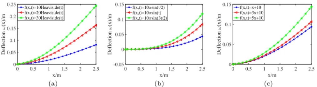
In this section, the displacements of HDPE rotating beam under different loads under FDKV model are discussed. When Ω = 0, there is no rotational force. Fig. 3 shows the displacements of the non-rotating beam under different uniform loads, simple harmonic loads and linear loads when t = 0.5s. Fig. 4 shows the displacements of HDPE rotating beam under different uniform loads, simple harmonic loads and linear loads when rotating speed Ω = π/2.
0 0.5 1 1.5 2 2.5 x/m 0 0.05 0.1 0.15 0.2 0.25 Deflection ω (x)/m f(x,t)=10Heaviside(t) f(x,t)=20Heaviside(t) f(x,t)=30Heaviside(t) (a) 0 0.5 1 1.5 2 2.5 x/m -0.05 0 0.05 0.1 0.15 Deflection ω (x)/m f(x,t)=10πsin(t/2) f(x,t)=10πsin(t) f(x,t)=10πsin(3t/2) (b) 0 0.5 1 1.5 2 2.5 x/m 0 0.05 0.1 0.15 Deflection ω (x)/m f(x,t)=x+10 f(x,t)=3x+10 f(x,t)=5x+10 (c)
Fig. 3. Displacements of HDPE non-rotating beams under different external loads: (a) Uniform loads; (b) Simple harmonic loads; (c) Linear loads.
0 0.5 1 1.5 2 2.5 x/m 0 0.1 0.2 Deflection ω (x)/m f(x,t)=10Heaviside(t) f(x,t)=20Heaviside(t) f(x,t)=30Heaviside(t) (a) 0 0.5 1 1.5 2 2.5 x/m -0.05 0 0.05 0.1 0.15 Deflection ω (x)/m f(x,t)=10πsin(t/2) f(x,t)=10πsin(t) f(x,t)=10πsin(3t/2) (b) 0 0.5 1 1.5 2 2.5 x/m -0.05 0 0.05 0.1 0.15 Deflection ω (x)/m f(x,t)=x+10 f(x,t)=3x+10 f(x,t)=5x+10 (c)
Fig. 4. Displacements of HDPE rotating beam at Ω =π
2 under different external loads: (a)
Uniform loads; (b) Simple harmonic loads; (c) Linear loads.
From Fig. 3, we can get that the displacements of the HDPE non-rotating beam gradually increases with time under the loads. At the same position, as the load increases, the displacement gradually increases. And the same conclusions can also be obtained by means of Fig. 4. In [49], a Fourier series is constructed and supplemented by a boundary smoothing term to express the displacement of the rotating beam. The governing equation of Ref.[49] can be considered as the governing Eq. (38) when α is fraction. Fig. 3 and Fig. 4 are similar to the results of Ref.[49]. Compared with Ref.[49], the numerical result is verified to be correct. In addition, we can clearly see that the displacements of HDPE beam changes with the rotation speed.
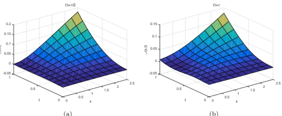
-0.05 1 0 0.05 2.5 ω (x,t) 0.1 2 Ω=π/2 t 0.15 0.5 1.5 x 0.2 1 0.5 0 0 (a) -0.05 1 0 2.5 0.05 ω (x,t) 2 Ω=π 0.1 t 0.5 1.5 x 0.15 1 0.5 0 0 (b)
Fig. 5. Displacements of HDPE rotating beam under external load f (x, t) = 10Heaviside(t)
at different rotational speeds: (a) Ω =π
2; (b) Ω = π.
Fig. 5 shows the numerical solutions of the displacement of the HDPE rotating beam at rotating speeds of Ω = π
2, Ω = π under the external load
f (x, t) = 10Heaviside(t). It can be seen from the image that the proposed
algorithm has a good simulation effect to solve such problems, and the feasibility of the algorithm is verified.
neu-tral surface can be expressed as:
ε = ∂
2ω(x, t)
∂x2 (57)
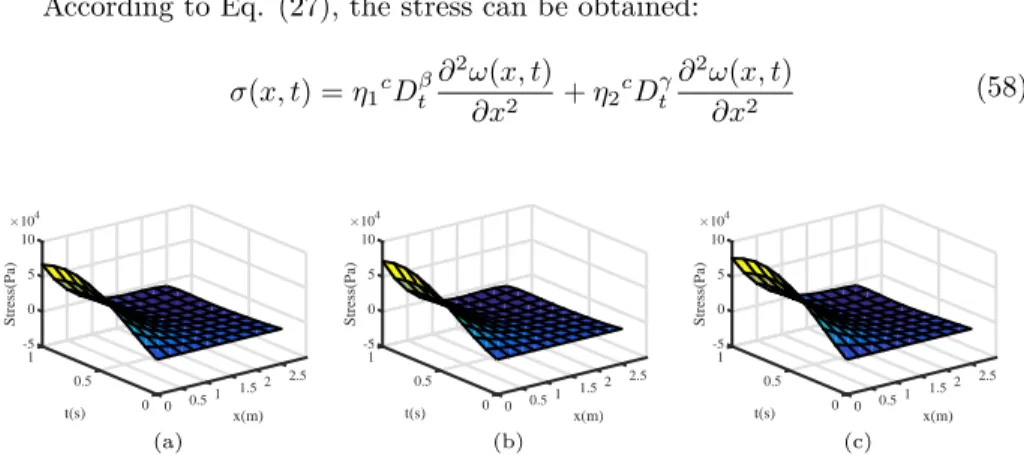
According to Eq. (27), the stress can be obtained:
σ(x, t) = η1cDβt ∂2ω(x, t) ∂x2 + η2 cDγ t ∂2ω(x, t) ∂x2 (58) -5 1 0 Stress(Pa) ×104 5 2.5 t(s) 0.5 2 x(m) 10 1.5 1 0.5 0 0 (a) -5 1 0 Stress(Pa) ×104 5 2.5 t(s) 0.5 2 x(m) 10 1.5 1 0.5 0 0 (b) -5 1 0 ×104 Stress(Pa) 5 2.5 t(s) 0.5 2 x(m) 10 1.5 1 0.5 0 0 (c)
Fig. 6. The stress of HDPE rotating beam at Ω = π
2 under different external loads: (a)
Uniform load f (x, t) = 10Heaviside(t); (b) Simple harmonic load f (x, t) = 10πsin(t); (c) Linear load f (x, t) = 10 + 2x.
Fig. 6 shows the stress of the HDPE rotating beam at the different external loads when the rotational speed Ω =π
2. Through the images, we can clearly see that the closer to the fixed end of the beam, the greater the stress. Therefore, the stronger the resistance to external force deformation near x = 0, the smaller the displacement. This is consistent with the change in the displacement map above. The accuracy and feasibility of the algorithm are further verified.
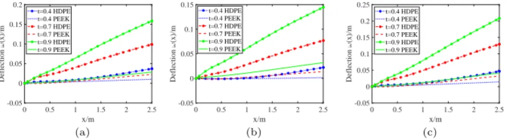
6.2. Comparison HDPE beams and PEEK beams
The displacement solutions of HDPE beam and PEEK beam under different loads of the FDE constitutive model are discussed and compared in this section.
0 0.5 1 1.5 2 2.5 x/m -0.05 0 0.05 0.1 0.15 0.2 Deflection ω (x)/m t=0.4 HDPE t=0.4 PEEK t=0.7 HDPE t=0.7 PEEK t=0.9 HDPE t=0.9 PEEK (a) 0 0.5 1 1.5 2 2.5 x/m -0.05 0 0.05 0.1 0.15 Deflection ω (x)/m t=0.4 HDPE t=0.4 PEEK t=0.7 HDPE t=0.7 PEEK t=0.9 HDPE t=0.9 PEEK (b) 0 0.5 1 1.5 2 2.5 x/m -0.05 0 0.05 0.1 0.15 0.2 0.25 Deflection ω (x)/m t=0.4 HDPE t=0.4 PEEK t=0.7 HDPE t=0.7 PEEK t=0.9 HDPE t=0.9 PEEK (c)
Fig. 7. Comparison of displacements between HDPE rotating beam and PEEK
non-rotating beam under different external loads: (a) Uniform load f (x, t) = 10Heaviside(t); (b) Simple harmonic load f (x, t) = 10πsin(t); (c) Linear load f (x, t) = 10 + 2x.
0 0.5 1 1.5 2 2.5 x/m -0.05 0 0.05 0.1 0.15 0.2 Deflection ω (x)/m t=0.4 HDPE t=0.4 PEEK t=0.7 HDPE t=0.7 PEEK t=0.9 HDPE t=0.9 PEEK (a) 0 0.5 1 1.5 2 2.5 x/m -0.05 0 0.05 0.1 0.15 Deflection ω (x)/m t=0.4 HDPE t=0.4 PEEK t=0.7 HDPE t=0.7 PEEK t=0.9 HDPE t=0.9 PEEK (b) 0 0.5 1 1.5 2 2.5 x/m -0.05 0 0.05 0.1 0.15 0.2 0.25 Deflection ω (x)/m t=0.4 HDPE t=0.4 PEEK t=0.7 HDPE t=0.7 PEEK t=0.9 HDPE t=0.9 PEEK (c)
Fig. 8. Comparison of displacements between HDPE rotating beam and PEEK rotating
beam at Ω = π
2 under different external loads: (a) Uniform load f (x, t) = 10Heaviside(t);
(b) Simple harmonic load f (x, t) = 10πsin(t); (c) Linear load f (x, t) = 10 + 2x.
Obviously, as can be seen from Fig. 7 and Fig. 8, the displacement of the PEEK beam is less than the displacement of the HDPE beam when the rota-tional speed and the external load are constant. The smaller the displacement, the greater the damping of the corresponding visco-elastic material and the better the bending resistance. Therefore, the PEEK beam have better bending resistance than the HDPE beam. The results obtained are consistent with the actual material properties. The proposed algorithm calculates the displacement solution well and has high precision. Thus, this method can provide a theoreti-cal basis for the research, development and performance prediction of damping materials.
7. Conclusion
In this paper, an effective numerical algorithm for solving fractional visco-elastic rotating beam based on SCPs is proposed for the first time in the time do-main. The displacements of visco-elastic beam can reflect the positional changes of beam at different times. The fractional derivative model is used to analyze the inherent laws of the dynamic performance of visco-elastic damping mate-rials, which can provide a theoretical basis for the research, development and performance prediction of damping materials.
1. Two governing equations of fractional visco-elastic rotating beam are es-tablished by FDE and FDKV constitutive models, the dynamic equation of beam and strain-displacement relationship.
2. According to the properties of SCPs, the integer and fractional differential operator matrices of polynomials are derived. Using the polynomial to ap-proximate the unknown function, the fractional order governing equation is rewritten into the form of matrix product. The variables are discretized based on the collocation method, and the original problem is transformed into an algebraic equation system. The numerical solutions of the govern-ing equations can be obtained directly in the time domain.
3. Numerical examples show the displacement and stress changes of HDPE rotating beam under uniform load, harmonic load and linear load un-der FDKV constitutive model, and further verify the effectiveness and
feasibility of the algorithm. By comparing the displacement of different viscoelastic beams, HDPE rotating beam and PEEK rotating beam, the properties of materials are analyzed theoretically.
Acknowledgments
This work is supported by the Natural Science Foundation of Hebei Province (A2017203100) in China and the LE STUDIUM RESEARCH PROFESSOR-SHIP award of Centre-Val de Loire region in France.
References
[1] Sweilam NH, Almekhlafi SM. Numerical study for multi-strain tuberculosis (TB) model of variable-order fractional derivatives[J]. Journal of Advanced Research. 2016, 7(2): 271–283.
[2] Ramirez, Coimbra. A variable order constitutive relation for viscoelastic-ity[J]. Annalen Der Physik. 2010, 16(7-8): 543–552.
[3] Lorenzo CF, Hartley TT. Initialization, conceptualization, and application in the generalized (fractional) calculus[J]. Critical Reviews in Biomedical En-gineering. 2007, 35(6): 447–553.
[4] Meerschaert MM, Scalas E. Coupled continuous time random walks in fi-nance[J]. Physica A Statistical Mechanics And Its Applications. 2006, 370(1): 114–118.
[5] Chen W. Nonlinear dynamics and chaos in a fractional-order financial sys-tem[J]. Chaos Solitons and Fractals. 2008, 36(5): 1305–1314.
[6] Du M, Wang Z, Hu H. Measuring memory with the order of fractional deriva-tive[J]. Scientific Reports. 2013, 3(7478):3431.
[7] Gemant A. On fractional differences[J]. Phil Mag. 1938, 25(1):92–96. [8] Bagley RL, Torvik PJ. On the fractional calculus model of viscoelasticity
behavior[J]. Journal of Rheology. 1986, 30(1):133–155.
[9] Leung AYT, Yang HX, Zhu P, Guo ZJ. Steady state response of fraction-ally damped nonlinear viscoelastic arches by residue harmonic homotopy[J]. Computers and Structures. 2013, 121(5):10–21.
[10] Lewandowski R, Pawlak Z. Dynamic analysis of frames with viscoelastic dampers modelled by rheological models with fractional derivatives[J]. Jour-nal of Sound and Vibration. 2011, 330(5):923–936.
[11] Kang JH, Zhou FB, Liu C, Liu YK. A fractional nonlinear creep model for coal considering damage effect and experimental validation[J]. International Journal of Non-Linear Mechanics. 2015, 76:20–28.
[12] Gioacchino A, Mario DP, Giuseppe F. On the dynamics of non-local frac-tional viscoelastic beams under stochastic agencies[J]. Composites Part B: Engineering. 2018, 131:102–110.
[13] Lewandowski R, Wielentejczyk P. Nonlinear vibration of viscoelastic beams described using fractional order derivatives[J]. Journal of Sound and Vibra-tion. 2017, 339(2):228–243.
[14] Lewandowski R, Baum M. Dynamic characteristics of multilayered beams with viscoelastic layers described by the fractional Zener model[J]. Archive of Applied Mechanics. 2015, 85(12):1793–1814.
[15] Cortes F, Elejabarrieta MJ. Finite element formulations for transient dy-namic analysis in structural systems with viscoelastic treatments containing fractional derivative models[J]. International Journal for Numerical Methods in Engineering. 2007, 69(10):2173–2195.
[16] Bahraini SMS, Farid M, Ghavanloo E. Large deflection of viscoelastic beams using fractional derivative model[J]. Journal of Engineering Mathe-matics. 2013, 27(4):1063–1070.
[17] Paola MD, Heuer R, Pirrotta A. Fractional visco-elastic Euler–Bernoulli beam[J]. International Journal of Solids and Structures. 2013, 50(22-23):3505– 3510.
[18] He XQ, Rafiee M, Mareishi S, Liew KM. Large amplitude vibration of fractionally damped viscoelastic CNTs/fiber/polymer multiscale composite beams[J]. Composite Structures. 2015, 131:1111–1123.
[19] Magdalena LP, Lewandowski R. Sensitivity Analysis of Dynamic Charac-teristics of Composite Beams with Viscoelastic Layers[J]. Procedia Engineer-ing. 2017, 199:366–371.
[20] Kiasat MS, Zamani HA, Aghdam MM. On the transient response of vis-coelastic beams and plates on visvis-coelastic medium[J]. International Journal of Mechanical Sciences. 2014, 83(7-8):133–145.
[21] Chang JR, Lin WJ, Huang CJ, Choi ST. Vibration and stability of an axially moving Rayleigh beam[J]. Applied Mathematical Modelling. 2010, 34(6):1482–1497.
[22] Friswell MI, Adhikari S, Lei Y. Vibration analysis of beams with non-local foundations using the finite element method[J]. International Journal for Numerical Methods in Engineering. 2007, 71(11):1365–1386.
[23] Demir DD, Bildik N, Sınır BG. Linear dynamical analysis of fraction-ally damped beams and rods[J]. Journal of Engineering Mathematics. 2014, 85(1):131–147.
[24] Permoon MR, Rashidinia J, Parsa A, Haddadpour H, Salehi R. Application of radial basis functions and sinc method for solving the forced vibration of fractional viscoelastic beam[J]. Journal of Mechanical Science and Technology. 2016, 30(7):3001–3008.
[25] Martin O. A modified variational iteration method for the analysis of vis-coelastic beams[J]. Applied Mathematical Modelling. 2016, 40(17):7988–7995. [26] Akritas P, Antoniou I, Ivanov VV. Identification and prediction of discrete chaotic maps applying a Chebyshev neural network[J]. Chaos, Solitons and Fractals. 2000, 11(1-3):337–344.
[27] Sun KK, Mou SS, Qiu JB, Wang T, Gao HJ. Adaptive Fuzzy Control for Non-Triangular Structural Stochastic Switched Nonlinear Systems with Full State Constraints[J]. IEEE Transactions on Fuzzy Systems. 2019, 27(8):1587– 1601.
[28] Qiu JB, Sun KK, Wang T, Gao HJ. Observer-Based Fuzzy Adaptive Event-Triggered Control for Pure-Feedback Nonlinear Systems with Prescribed Per-formance[J]. IEEE Transactions on Fuzzy Systems. 2019, 27(11):2152–2161. [29] Qiu JB, Sun KK, Rudas IJ, Gao HJ. Command Filter-Based Adaptive
NN Control for MIMO Nonlinear Systems With Full-State Constraints and Actuator Hysteresis[J]. IEEE Transactions on Fuzzy Systems. 2019, 1–11. [30] Tadjeran C, Mark M. Meerschaert and Hans-Peter Scheffler. A second-order
accurate numerical approximation for the fractional diffusion equation[J]. Journal of Computational Physics. 2006, 213(1):205-213.
[31] Meng ZJ, Yi MX, Huang J, Lei S. Numerical solutions of nonlinear frac-tional differential equations by alternative Legendre polynomials[J]. Applied Mathematics and Computation. 2018, 336:454–464.
[32] Chen YM, Sun YN, Liu LQ. Numerical solution of fractional partial dif-ferential equations with variable coefficients using generalized fractional-order Legendre functions[J]. Applied Mathematics and Computation. 2014, 244(2):847–858.
[33] Xie JQ, Yao ZB, Gui HL, Zhao FQ, Li DY. A two-dimensional Chebyshev wavelets approach for solving the Fokker-Planck equations of time and space fractional derivatives type with variable coefficients[J]. Applied Mathematics and Computation. 2018, 332:197–208.
[34] Chen YM, Sun L, Li X, Fu XH. Numerical solution of nonlinear fractional integral differential equations by using the second kind Chebyshev wavelets[J]. Computer Modeling in Engineering and Sciences. 2013, 90(5):359–378. [35] Wang J, Xu TZ, Wei YQ, Xie JQ. Numerical solutions for systems of
frac-tional order differential equations with Bernoulli wavelets[J]. Internafrac-tional Journal of Computer Mathematics. 2018, 96(2):317–336.
[36] Chen YM, Liu LQ, Liu DY, Boutat D. Numerical study of a class of vari-able order nonlinear fractional differential equation in terms of Bernstein polynomials[J]. Ain Shams Engineering Journal. 2016,1235–1241.
[37] Chen YM, Liu LQ, Li BF, Sun YN. Numerical solution for the variable or-der linear cable equation with Bernstein polynomials[J]. Applied Mathematics and Computation. 2014, 238(7):329–341.
[38] Fernanda SP, Miguel P, Higinio R. Extrapolating for attaining high pre-cision solutions for fractional partial differential equations[J]. Fractional Cal-culus and Applied Analysis. 2018, 21(6):1506–-1523.
[39] Suman S, Kumar A, Singh GK. A new method for higher-order linear phase FIR digital filter using shifted Chebyshev polynomials[J]. Signal Image and Video Processing. 2016, 10(6):1041–1048.
[40] Zaicenco AG. Sensitivity analysis of a seismic risk scenario using sparse Chebyshev polynomial expansion[J]. Geophysical Journal International. 2015, 200(3):1466–1482.
[41] Xing S, Guo HW. Temporal phase unwrapping for fringe projection pro-filometry aided by recursion of Chebyshev polynomials[J]. Applied Optics. 2017, 56(6):1591–1602.
[42] Protasov V, Jungers R. Analysing the Stability of Linear Systems via Expo-nential Chebyshev Polynomials[J]. IEEE Transactions on Automatic Control. 2016, 61(3):795–798.
[43] Srivatsa BK, Ganguli R. Non-rotating beams isospectral to rotating Rayleigh beams[J]. International Journal of Mechanical Sciences. 2018, 142-143:440–455.
[44] Tian JJ, Su JP, Kai Z, Hua HX. A modified variational method for nonlin-ear vibration analysis of rotating beams including Coriolis effects[J]. Journal of Sound and Vibration. 2018, 426:258–277.
[45] Bazoune A. Effect of tapering on natural frequencies of rotating beams[J]. Shock and Vibration. 2014, 14(14):169–179.
[46] Banerjee JR, Su H, Jackson DR. Free vibration of rotating tapered beams using the dynamic stiffness method[J]. Journal of Sound and Vibration. 2006, 298(4):1034–1054.
[47] Xu HY, Jiang XY. Creep constitutive models for viscoelastic materials based on fractional derivatives[J]. Computers and Mathematics with Appli-cations. 2017, 73(6):1377–1384.
[48] Lin YM, Xu CJ. Finite difference/spectral approximations for the time-fractional diffusion equation[J]. Journal of Computational Physics. 2007, 255(2):1533–1552.
[49] Chen Q, Du JT. A Fourier series solution for the transverse vibration of rotating beams with elastic boundary supports[J]. Applied Acoustics. 2019, 155:1–15.