Design Tools and Mechanisms for Progressive
Cavity Pumps
by
Kevin P. Simon
B.S., Franklin W. Olin College of Engineering (2012)
S.M., Massachusetts Institute of Technology (2015)
Submitted to the Department of Mechanical Engineering
in partial fulfillment of the requirements for the degree of
Ph.D. in Mechanical Engineering
at the
MASSACHUSETTS INSTITUTE OF TECHNOLOGY
February 2019
Massachusetts Institute of Technology 2019. All rights reserved.
Author ...
Certified by...
Signature redacted
Department of Mechanical Engineering
November 20, 2018
Signature redacted_____,
Alexander H. Slocum
Walter M. May & A. Hazel May Professor of Mechanical Engineering
Thesis Supervisor
Accepted by.
OFTEHNOLYFEB' 25 2019
LIBRARIES
Signature redacted
...
. .
Nicolas Hadjiconstantinou
Chairman, Department Committee on Graduate Theses
Design Tools and Mechanisms for Progressive Cavity Pumps
by
Kevin P. Simon
Submitted to the Department of Mechanical Engineering on November 20, 2018, in partial fulfillment of the
requirements for the degree of Ph.D. in Mechanical Engineering
Abstract
This thesis presents tools to design progressive cavity pumps (PCPs), with an em-phasis on low-viscosity fluids. These models indicate that high speed operation can increase sealing performance, decrease pump size, and eliminate gear-reductions. New models for estimating both laminar and turbulent internal flow and shear losses in these pumps are presented. The new models are capable of estimating pump perfor-mance 1000x faster than traditional simulation methods, and do not require empirical calibration, making them 'designer-ready'. A proof-of-concept turbulent PCP was de-signed using these models. Its volumetric efficiency is within 20% of predicted values. This thesis also presents a novel one degree-of-freedom hypocycloidal bearing to constrain the motion of the rotor for increased performance and control. 3 different bearing topologies have been developed: roller, rail, and flexural. An experimental PCP concept with integrated hypocycloidal rail bearings was developed and tested with efficiencies as high as 45%. Experimental data are compared with a new lubrica-tion theory model which accounts for rotor molubrica-tion, rotor geometric error, and stator geometric error. The experimental and theoretical results show strong agreement, proving that low-order lubrication theory models are accurate simulation tools.
Additionally, performance results from the rail bearing pump and first-order anal-ysis inspire new scaling laws for connecting the volumetric and mechanical efficiency of PCPs. These scaling laws show strong agreement in both turbulent and laminar
flows.
A new generation of PCPs has the potential to transform irrigation, water
purifica-tion, oil-sand extracpurifica-tion, among other applications. The new tools required to create these PCPs also have strong implications for how traditional PCPs are designed. Thesis Supervisor: Alexander H. Slocum
Acknowledgments
This thesis was made possible by support from the MIT Tata Center, the Tata Trusts, the Martin Family, and the Abdul Latif Jameel Water & Food Systems Lab. I also want to acknowledge the Ann Goss Foundation for providing me the Jackson W. Goss Fellowship to help build Khethworks in the Martin Trust Center's Global Founders' Skills Accelerator during the summer of 2015. I particularly want to thank the MIT Tata Center. Not only did they sponsor 4 of my years in grad school. The 12 trips to India, connections, and faith in the potential of my pump work was essential to this project.
Thank you Prof. Slocum for your faith in my skills while constantly injecting non-linear genius to my process. You've been a world-class advisor.
Mom, Julia, and Dad: thank you for everything that you have done to support,
care for, and teach me. You were my first champions, and I would not be 'here' without you.
I am deeply grateful to my partner, Hilary White. Your love, support, and patience
in the last 5 years mean the world to me.
One of the most essential ingredients for good research is a thriving intellectual community. While the nature of a thesis is individual, this work would have been impossible without the wisdom, knowledge, and support of my colleagues at MIT and elsewhere. Thank you David, Hilary, Abe, Marcel, Thanh, Tyler, and Lei. It is impossible for me to thank and account for every person who has shaped this thesis. You all in particular have critically influenced this work. PERG and Makerworks have been cornerstones of my MIT experience, and I am deeply grateful for those groups of wonderful individuals.
The data presented in this thesis would not have been possible without the help of Aaron Johnson's CT stator scanning at Amphenol TCS; Nick Sondej's 3D rotor scanning; David Taylor's data collection code; or Aaron Ramirez's help instrumenting my torque sensor. Thank you so much for your help.
Contents
1 Introduction 27
1.1 Motivation . . . . 28
1.2 PCP Principles . . . . 29
1.3 Why PCPs? . . . . 30
1.4 Goals of this Research . . . . 32
1.5 PCP Literature Review . . . . 34
1.5.1 Experiments . . . . 34
1.5.2 M odels . . . . 34
1.5.3 D esign . . . . 36
1.5.4 Water Applications . . . . 37
2 Lubrication Theory and Geometric Errors 39 2.1 Lubrication Theory Model . . . . 39
2.1.1 Derivation and Clarifications . . . . 39
2.1.2 Numerical Implementation . . . . 46
2.2 Modeling Geometric Error in PCPs . . . . 48
2.2.1 Imperfect Rotor and Stator Model . . . . 50
2.2.2 Rotor Surface Error . . . . 50
2.2.3 Rotor Error Motion . . . . 51
2.2.4 Stator Surface Error . . . . 58
2.3 Internal Forces . . . . 60
2.3.1 Torque Scaling . . . . 60
2.4 Implications for Qth . . . . 2.5 Conclusions . . . .
3 Turbulence in Progressive Cavity Pumps
3.1 Network M odels . . . .
3.1.1 Background . . . .
3.1.2 Extension of Network Model . . . .
3.1.3 Model Validation . . . .
3.1.4 Combined Turbulent and Lubrication Flow
3.2 RANS Turbulence Models . . . .
3.2.1 Turbulence Model Application . . . .
3.2.2 Inclusion of Cell-Averaged Inertial Terms .
Resistance
3.3 Conclusions . . . . 4 PCP Design
4.1 1-DOF Cycloidal Bearing Design 4.1.1 Orbiting Strategy... 4.1.2 Hirth Coupling Assembly. 4.2 Rolling Bearing Experiment . . .
4.2.1 M otor . . . . 4.2.2 Sensors . . . . 4.2.3 Total Design . . . . 4.2.4 Cavitation . . . . 4.2.5 Results . . . . 4.3 Rail Bearing Experiment...
4.3.1 Structure Design... 4.3.2 M otor . . . . 4.3.3 Sensors . . . . 4.3.4 Total Design . . . . 4.3.5 Results . . . . 4.4 Water PCP Concept . . . . 69 72 75 76 76 80 86 89 91 91 95 96 97 97 108 109 110 111 112 112 116 118 119 120 121 121 125 129 142
5 Conclusion 145 5.1 R em arks . . . . 145
List of Figures
1-1 PCP rotor (left), stator (right), and cavities (bottom). . . . . 28
1-2 A depiction of typical PCP geometry from the side (left) and in cross-section (right). . . . . 29 1-3 The clearance gap within a progressive cavity pump. The rotor has
six pitches over its 0.36 m length with a rotor radius of 0.020 m. The yellow regions correspond to cavities. . . . . 31
1-4 The ranges of flow applications where pumping technologies are cost effective, compared to the requirements of irrigation and water purifi-cation . . . . 32
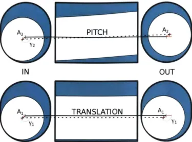
2-1 Different zones of the stator relative to the center of the rotor, adapted from Andrade et al. [3]. . . . . 41 2-2 The critical dimensions of a PCP viewed from the side (left) and outlet
(right). . . . . 43
2-3 A representation of the numerical grid used to evaluate the Poisson
pressure equation. Each node (O,z) corresponds to a point where the pressure is evaluated. . . . . 47 2-4 Net flow rate at different sections as a measure of conservation of mass
for a centered grid (left) and a staggered grid (right) . . . . 48
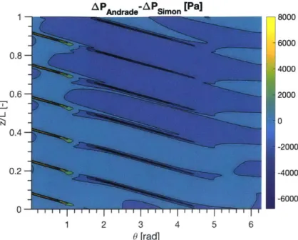
2-5 The pressure difference between Andrade's results and the model in
this paper on a grid where n2 = 500 and no = 250. . . . . 49
2-6 An example of sinusoidal surface error on the rotor. (Ae = 185 pm,
2-7 Geometric definitions of the two motion-driven error modes. . . . . . 52 2-8 Time averaged flow rates for different surface error amplitudes and
spatial frequencies (n=m=1 to n=m=10). The mesh was created with 1400 nodes in z and 400 nodes in 0 to resolve the spatial frequencies. 53
2-9 A two dimensional depiction of rotor error motion. . . . . 53
2-10 An example of rotor radius changes corresponding to small angle rotor
motion. (A1 = 83 pm, A2 = 83 im, '1 = 0, '72 = 7r/2) . . . . 54
2-11 Experimental results from Gamboa with 0.042 Pa-s oil compared with Andrade's centered rotor lubrication theory model and the rotor error motion uncertainty presented in this thesis [18, 3]. . . . . 55
2-12 Experimental results from Gamboa with 0.134 Pa-s oil compared with Andrade's centered rotor lubrication theory model and the rotor error motion uncertainty presented in this thesis [18, 3]. . . . . 56 2-13 Experimental results from Gamboa with 0.481 Pa-s oil [18]. The
theo-retical flow-rate for this pump, Qth, is 5.39 m3
/s.
Both theexperimen-tal data and skewed-rotor model have flow-rates greater than Qth. . . 57
2-14 Rail bearing experimental results and lubrication theory simulation based on rotor and stator scans. ... ... 58 2-15 Gamboa's experimental results compared with CFD simulation by
Pal-adino [19, 44]. . . . . 59 2-16 The sensitivity of 2D lubrication theory and 3D CFD simulations to
grid size. 2-D lubrication theory has a much faster convergence rate than conventional CFD. . . . . 60 2-17 Comparison between Vetter's experiment and lubrication theory with
a corresponding turbulent viscosity. . . . . 70 2-18 Lubrication theory results compared with the Paladino CFD for the
same geometry (botton) [44. Simulated (left) and experimental (right) torques from this work. . . . . 71
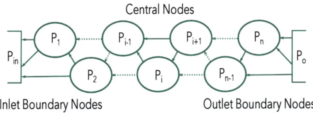
3-2 Illustration of the cavity nodes and connectivity in a PCP network model. The arrows represent slip flow between cavities. . . . . 80 3-3 Pressure distribution along the rotor of a representative 2 cavity pump.
Transverse sealing lines connect cavities that are two nodes apart, and are horizontal lines above. Longitudinal sealing lines connect neigh-boring cavities, and appear at an angle above. . . . . 81
3-4 The effect of different geometric variables on the longitudinal pres-sure loss coefficient. Higher values of K/K indicate better geometry-independent sealing and delayed transition to turbulence. . . . . 87 3-5 Results from the orifice network model compared with experimental
data from Gamboa and Vetter [19, 57] . . . ... 88 3-6 Results from the water prototype plotted against predictions from the
orifice network model. Black lines connect experimental data and sim-ulation results at the same speed and pressure. . . . . 88
3-7 A viscous channel followed by a mixing dominated sudden expansion. 89
3-8 Results from the long orifice network model compared with experimen-tal data from Gamboa and Vetter [19, 57]. . . . . 90 3-9 Results from the water prototype plotted against predictions from the
long orifice network model. Black lines connect experimental data and simulation results at the same speed and pressure. . . . . 91
4-1 Example pressure distribution over a water hydrodynamic bearing, computed using lubrication theory. In this case, L = 20 mm, Rj =
15 mm. c = 20 pm, e = 10 pm, and Q = 419 rad/s . . . . 100
4-2 Front view of the CAD for the vertical (left) and horizontal (left) flex-ural hypocycloidal crankshaft bearing stages. . . . . 103
4-3 Energy stored in the othrogonal flexure system. . . . . 104 4-4 Angled view of a flexural hypocycloidal crankshaft bearing. . . . . 105
4-5 The dynamic response of the under-constrained floating stage . . . . 107
4-7 Image of the water pump crank assembly with one of the Hirth cou-plings visible from the side. . . . 109 4-8 Sectioned view of the water pump hypocycloid bearing and crank shaft
rotor.. ... ... . ... . . . . ... 111
4-9 Sectioned and whole views of the water pump assembly CAD. . . . . 114 4-10 Picture of the full water pump assembly. . . . . 115
4-11 Image of the crankshaft rotor (top). Close up of the inlet side (left) and outlet side (right) of the crank with roller bearings and axial support b all. . . . . 115
4-12 Cavitation on the inlet side of the water prototype rotor due to incor-rectly designed PCP inlet conditions. . . . . 116
4-13 Section view of the PCP inlet and inlet bearings with the side inlet (top), and the axial inlet (bottom). . . . . 118
4-14 Results from the water prototype plotted against predictions from the orifice network model. Black lines connect experimental data and sim-ulation results at the same speed and pressure. . . . . 119
4-15 Sectioned isomeric view of the rail bearing pump outlet with ball gear joint, outlet bearings, and eddy current probe CAD (left). Assembled ball gear joint (right) . . . . 121 4-16 The residual from fluid accelerations for the highest flow-rate
experi-ment. This residual at most is 3% of the nominal pressure. . . . . 123
4-17 The pressure loss coefficient computed for various needle-valve posi-tions in the flow loop . . . . 124 4-18 CAD cross-section (top left) alongside a picture (top right) of the
drive-shaft end of the rotor inside the stator with an eddy-current target (yellow in the CAD, and aluminum in the picture) attached. CAD cross-section of the inlet end of the rotor inside the stator with an eddy-current target attached (bottom left)alongside a picture of the eddy-current probe placement on one end of the stator (bottom right). 126 4-19 Whole and sectioned views of the rail bearing pump assembly CAD. . 127
4-20 Image of the assembled rail-bearing pump with flow loop. . . . . 128
4-21 Close up of the rotor inside of the clear stator. . . . . 128
4-22 Sectioned isomeric view of the rail bearing pump inlet with ball drive, outlet bearings, and eddy current probe CAD (left). Assembled rail bearing prototype (right). . . . . 128
4-23 lubrication theory simulation results alongside flow rates from the rail bearing prototype experiment. . . . . 129
4-24 Efficiencies from the rail bearing prototype experiment. Volumetric efficiency, mechanical efficiency, and total efficiency are o, o, and x respectively . . . . 130
4-25 Measured shaft torque from the rail bearing prototype experiment (left) and lubrication simulation torques (right). . . . . 131
4-26 Scaling model for PCP efficiency compared with experimental data for volumetric efficiency (o), mechanical efficiency (o), and total efficiency
(x). ... ... 132
4-27 Scaling model for PCP efficiency compared with experimental data from the water prototype. . . . . 133
4-28 The simple single quadratic resistor slip flow relationship used in the turbulent scaling laws compared with experimental results and the ori-fice network model. Black lines connect experimental data and simu-lation results at the same speed and pressure. . . . . 134 4-29 Estimates of motor torque from the water (+) prototype experiment
and scaling law fit (*). Black lines connect experimental data and simulation results at the same speed and pressure. . . . . 135
4-30 A comparison of similar turbulent and laminar pumps to illustrate the effect of turbulent sealing. . . . . 136
4-31 The flow (left) and pressure (right) signal overlaid in the same time window with the valve 1.5 turns open. . . . . 139
4-32 The torque (left) and probe (right) signal overlaid in the same time window with the valve 1.5 turns open. . . . . 139
4-33 Torque (left) and pressure (right) measurements for the rail bearing prototype running at 200 rpm with mineral oil at various valve posi-tions. The grey line at the bottom of the torque measurements is a kinematically repeatable parasitic torque that was measured by run-ning the pump with only enough working fluid to lubricate the rotor. 140 4-34 Circumferential distribution of deviations from the stator's internal
designed geometry (left), and the rotor radius (right). . . . . 141 4-35 The effect of stator and rotor error on the pressure fluctuations
assum-ing a laminar flow loop pressure drop. . . . . 142 4-36 Estimated flow rates for the water PCP concept proposed (left) and
the hypothetical efficiency curve for the water PCP concept (right). 143
List of Tables
2.1 R, values in different regions of the PCP. These are updated to correct for some typos in Andrade's original work
[3].
. . . . 42 2.2 OR0 values in different regions of the PCP. These are updated to correctfor some typos in Andrade's original work [3]. . . . . 43
2.3 Simulation runs to illustrate flow and rotor dynamics. . . . . 72
3.1 The pressure profiles of different PCP models for the 4 sealing cavity PCP. The linear models were calibrated against a two cavity PCP lubrication simulation, and were simulated with Re ~ 50. . . . . 86
4.1 Critical design dimensions of the water prototype . . . . 113
Nomenclature
cI Angle defining stator region I [rad]
&2 Angle defining stator region II [rad]
Tcy1 Fluid shear stress tensor in cylindrical coordinates [Pa]
7 Total fluid shear stress in cartesian coordinates [Pa]
Tf Reference frame shear stress [Pa]
1 Cumulative flow [m3
]
A Pressure matrix [Pa] R Rotation matrix
[-]
AP Static pressure rise [Pa]APL Laminar sealing line static pressure drop [Pa]
APT Transverse sealing line static pressure drop [Pa]
APTL Long orifice static pressure drop [Pa]
A Driven stage displacement [im]
6 Flexure displacement [im]
6 Surface roughness [m]
7 Total PCP efficiency [-]
TIL Total PCP efficiency for laminar operation (from scaling laws) [-]
r/M Mechanical efficiency [-]
r'v Volumetric efficiency [-]
rqm, Motor controller efficiency [-]
71 Meridional angle of the rotor error translation [rad]
72 Meridional angle of the rotor error pitch [rad]
w Nominal clearance gap [m]
P Coefficient of friction for the Hirth coupling (Section 4.1.2) [-1
P Dynamic viscosity [Pa-s]
Pt Effective turbulent eddy viscosity [Pa-s]
v Kinematic viscosity [m2/s]
v Poisson ratio (Chapter 4) [-]
Q Rotational velocity [rad/s]
Q* Dimensionless rotational velocity [rad]
we Critical speed for shaft whip [rad/s]
p Fluid density [kg/M3] Ub Flexure bending stress [Pa]
T Torque [N-m]
TK Flow meter time constant [pulses/s] TO Parasitic torque [N-m]
0 Circumferential coordinate [rad]
Es
Angle between the stator section centerline and the horizontal plane [rad] n Rotor surface normal [-]V Rotor surface velocity [m/s]
A Angle between stator regions I and III (Chapter 2) [rad]
A Fluid resistor matrix coefficient [im3/Pa-s]
A' Angle between stator regions I and IV [rad] 20
A1 Amplitude of the rotor error translation [m] A2 Amplitude of the rotor error pitch [m] Ae Surface error amplitude [m]
Af Driven stage displacement amplitude [m]
B Angle between stator regions II and III [rad]
b Sealing line width [m]
B' Angle between stator regions II and IV [rad]
biong Longitudinal sealing line width [m]
btrans Transverse sealing line width
[m]
c Nominal journal bearing clearance height
[m]
C1 Circumferential coefficient of integration [m2/Pa-s]
C1 Coefficient of integration (Chapter 4) [m]
C2 Axial coefficient of integration [m4/Pa-s]
C2 Coefficient of integration (Chapter 4) [m] Cd PCP modulus of drag [N-m s/rad]
Cf PCP coefficient of friction [-]
C, Pressure loss coefficient [-]
CQ PCP flow modulus [m3/rad]
CR Flow resistance modulus [Pa-s/m3l
Cow Coefficient of integration [m2/s]
c~r PCP torque modulus [m3]
CpL Laminar pressure loss coefficient [-]
CpT Turbulent pressure loss coefficient
[-]
CsL PCP laminar slip modulus [m3/Pa-s]
D Plate stiffness [N-m]
Df Hydraulic diameter [im]
Dh Hydraulic diameter [m]
dcsR Distance between the center of the stator and the center of the rotor [m]
dA Surface area differential [m2
]
E Young's modulus (Chapter 4) [Pa]
e Journal bearing eccentricity [im]
Ef Flexural energy [J]
Eotat Total Hirth coupling stiffness [N/m]
Ek Ekman number
[-]
f Friction factor [-]
Ff Applied flexure force [N]
Fp Hirth coupling preload force [N]
FT Tangential Hirth coupling force [N]
Fc, Critical flexural buckling load [N]
g Gravitational acceleration at the surface of the earth [m/s2
]
h Journal bearing clearance height [m]
I Current [A]
I Flexure second moment of area [m4]
I,, No-load current [A]
K Laminar viscous coefficient [-]
K Simplifying coefficient (Chapter 2) [-]
k Flexure stage stiffness [N/m]
Kb Buckling coefficient [-]
KL Longitudinal laminar viscous coefficient
[-)
Km Flow meter K-factor [m3
/pulse]
KT Transverse laminar viscous coefficient
[-3
Kt Motor torque constant [V-s/rad]
K, Motor voltage constant [rad/V-s]
kv Vertical flexure stiffness [N/m]
L Longitudinal cavity fluid conductivity [m3/Pa-s]
L PCP rotor length (used for non-dimensionalization in figures) [m]
I Length of the rotor
[ml
L* Dimensionless longitudinal cavity fluid conductivity
[-3
if Flexure length [m]
is Effective sealing line length [m]
M Flexure bending moment [N-m]
M Floating stage mass [kg]
m Rotor mass (Chapter 4) [kg]
m Surface error spatial frequency in z (Chapter 2)
[-]
n Surface error spatial frequency in 0[-]
No Number of grid cells in 0 [-]
np Number of parallel flexure stages
[-]
N2 Number of grid cells in z [-]
P Motor power [W]
p Static pressure [Pa]
P1 First cavity relative static pressure [Pa]
P2 Second cavity relative static pressure [Pa]
P Relative static outlet pressure [Pa]
Pr Nominal rotor pitch [m/rev]
P, Nominal stator pitch [m/rev]
Prot Rotor input power [W]
Q
m Lubrication theory model predicted flow rate [m3/s]Qexp Experimentally measured flow rate [m3/s]
Qthr Maximum flow rate, computed from the rotor geometry [m3
/s]
Qth, Maximum flow rate, computed from the stator geometry [m3/s]Qth Theoretical maximum flow rate (could use Qths or Qthr) [m3/S]
R Resistance (Chapter 4) [Ohm]
r Radial coordinate [m]
RI Journal bearing radius [m]
RL Longitudinal cavity sealing resistance [Pa-s/m3]
Ro Radial distance between the center of the rotor and the wall of the stator [im]
Rr Nominal rotor radius [im]
Rs Nominal stator radius [m]
RT Transverse cavity sealing resistance [Pa-s/m3] R,li Total pump slip flow resistance [Pa-s/m3]
Ro Rossby number [-]
S Rotor surface coordinate (Chapter 2) [m]
S Slip flow rate [m3/s]
SL Laminar slip flow rate [m3/s]
ST Turbulent slip flow rate [m3/s]
Scr Rotor center coordinate [i]
t Time [s]
T* Dimensionless transverse cavity fluid conductivity
[-]
U Slip flow speed [m/s]
u Axial fluid velocity [m/s]
V Voltage [V]
v Radial fluid velocity [m/s] Vf Reference frame velocity
[m/sj
w Tangential fluid velocity [m/s]Wf Flexure width [m]
z Axial coordinate [im]
AR Area ratio [-]
E Rotor eccentricity [im]
errm Rotor error motion magnitude
[m]
errs Surface error magnitude [m]
Chapter 1
Introduction
There are many types of pumps for moving fluids and gases, and societies of any type critically depend on them. The use of pumps for irrigation and drinking water is among the oldest applications of engineering. One of the first pumps, the shadoof, was documented in the city of Uruk, in what is now Iraq, around 3,300 BC [58]. Denis Papin invented the world's first true centrifugal pump in 1687 [62]. In the meantime, the role of pumps in irrigation has grown significantly. In 2016 the agricultural sector in India consumed 173 TWh of energy [31]. Much of that energy was used for irrigation. In spite of the maturity and importance of this field, there is still a gap in the use of electrical power for irrigation or the production of drinking water. This problem is acutely relevant in developing countries. For example, East India has among the highest 'fraction of rural persons going hungry' in India [12]. Tragically, this is a region where many agricultural fields lay un-used for over half of the year because of a lack of access to affordable irrigation and market linkages. Ending hunger and providing access to clean water are both UN Sustainable Development Goals [17]. Providing access to clean water, and making solar energy economical are both NAE Grand Challenges [46]. Creating more efficient low-energy water pumps is directly relevant to these broad societal goals.
Figure 1-1: PCP rotor (left), stator (right), and cavities (bottom).
1.1
Motivation
This research was initially motivated by the author's work with small plot farmers in East India as part of a Tata-trusts sponsored fellowship [49]. Agriculture is a major source of livelihood for over 300 million farmers in India. In the summer, farmers are able to rely on the monsoon rains to irrigate their crops, but winter and dry-season farming require irrigation. Some farmers have the benefit of canals, but the majority of farmers in India depend on groundwater for irrigation. Even though there is considerable growth in groundwater usage, the cost of pumping water and access to energy often makes year-round irrigation unfeasible for these farmers. Many small plot farmers use costly and polluting diesel powered pumps to irrigate their fields. Current irrigation technologies are not accessible for the majority of Indian farmers. Over 50% of all cropped land in India is unirrigated [1]. Where there is access to electricity, the subsidized agricultural load on India's electricity grid is costly and decreases the hours of available energy for other uses. In the 2015-2016 season, agricultural irrigation accounted for 17.3% of electrical power consumption in India [31].
Increasing the efficiency of groundwater pumps has the ability to save government money on energy subsidy programs; increase the quality of grid operations; enable year-round irrigation; and enable solar irrigation to compete with diesel pumps. This improvement could be realized by creating better positive displacement pumps, which has the potential to be more efficient than centrifugal pumps for the pressure rise
(100-350 kPa) and flow rate (1-2 lps) requirements of these farmers.
1.2
PCP Principles
The progressive cavity pump (PCP) was invented in 1930 by Moineau and presented in his doctoral thesis [36]. Some authors refer to them as progressing cavity pumps, but this thesis will exclusively use 'progressive cavity pumps'. PCPs are rotary positive displacement pumps with a single helix rotor eccentrically rotating in a hypocycloidal trajectory inside of a double helix stator. Multiple helix PCPs do exist, but that ge-ometry is most commonly used in 'mud-motors.' This work focuses exclusively on single helix PCPs. An example of the geometry, and the respective cavities, contain-ing discrete volumes of fluid, are shown in Fig. 1-1. Those cavities spiral along the axis of the pump. PCPs are commonly used in chemical processing and oil and gas applications because of their efficiency and ability to handle high viscosity fluids and mixed phase flows. Even though the pumps have no valves and few components, cur-rent PCPs are too expensive for use in irrigation due to the manufacturing tolerances of the rotor and stator. Beyond price concerns, the efficiency of PCPs is driven by slip flow along sealing clearance lines. This slip flow rate is proportional to the viscosity of the fluid, which makes designing PCPs for water particularly challenging.
PS
4E
R.
Pr-Figure 1-2: A depiction of typical PCP geometry from the side (left) and in cross-section (right).
Each cavity progresses along the axis of the PCP at a rate that is set by the rotor speed and pitch. The product of axial cavity velocity and the cross-section of the pump are the basis of Eq. 1.1, an estimate for the ideal flow-rate if there is no slip flow [47, 57, 39]. E is the eccentricity of the spirals. R, is the radius of the rotor. R,
is the radius of the stator. P, is the pitch of the stator, typically expressed in units of [m/rev]. P, is the pitch of the rotor, which is half of the pitch of the stator. Q is the rotational speed of the rotor. Unless otherwise indicated, Q is expressed in S.I. units, [rad/s]. These geometric terms are shown in detail in Fig. 1-2.
Qths = [8E R, + r(R 2 - R ,2)]
(1.1
27r
Another, less common, estimate for the maximum theoretical flow-rate of a PCP,
Eq. 1.2, is based on the area that the rotor sweeps out [4].
Qthr = -ERrPQ (1.2)
7r
The clearance can be visualized for an example pump geometry (6 pitches, 0.36 m long, rotor radius of 0.02 m, stator radius of 0.020185 m, eccentricity of 0.004039 m) in Fig. 1-3. This is the geometry of the pump used in experiments by Gamboa et al., which are commonly used to validate PCP models [19, 43, 3, 11, 47]. While the rotor-stator clearance in rigid stator PCPs gets to be small between the cavities, it is never zero, as seen in Fig. 1-3. It follows that the pressure difference between the cavities creates back-flow along those clearance lines, visualized in Fig. 1-2, which reduces the pump's volumetric efficiency. The shaft-to-flow efficiency of a PCP is the product of volumetric efficiency and mechanical efficiency.
1.3
Why PCPs?
This thesis focuses on PCPs for two reasons. Progressive cavity pumps have ex-ceptional flow characteristics: they have the advantages that positive displacement pumps have over centrifugal pumps at high pressure differences and low flow rates (i.e. low specific speeds) without the challenges that most positive displacement pumps have with valving, flow pulsations, handling solids, or complexity.
Centrifugal pumps reduce in efficiency with specific speed and with flow rate [28]. One highly optimized centrifugal pump, with a still greater specific speed than the
Rotor-Stator Clearance [ml 0 .3 5 1 4 0.3 .12 0.25 10 0.2 8 N 0.15 6 0.14 0.05 2 0 1 2 3 4 5 6 Theta [rad]
Figure 1-3: The clearance gap within a progressive cavity pump. The rotor has six pitches over its 0.36 m length with a rotor radius of 0.020 m. The yellow regions correspond to cavities.
applications considered in this thesis, reaches a maximum efficiency of 60%. However, the designer of that pump notes that with increasing pressure., the efficiency of the pump would be reduced considerably [10].
In spite of these properties, PCPs are mainly used in oil and gas, sewage., and chemical processing because of the high cost of precision manufacturing for the com-plex shapes. As such, there is limited literature on applications outside of oil and gas. When this thesis was written, there was not enough literature for an engineer skilled in the art of fluid machinery design to quickly and easily do early stage design or evaluation the feasibility of a water-moving PCP. Most low-order models are tailored to high viscosity fluids; all models assume that manufacturing is arbitrarily precise; and many models have ambiguities that make it difficult for a designer to quickly implement them.
It is this author's belief that there are, as yet, un-designed PCPs with the potential to improve water delivery and purification. Figure 1-4 qualitatively shows what this design space could look like. There are likely other existing applications for PCPs beyond those as well. The lack of literature on this subject; the magnitude of current water-related challenges; and the fundamental advantages of PCPs justify a
centric research effort to expand the world of possibilities for PCPs working with water.
Cost Effectiveness
New PCP Tech
Irrigation +
Purification
nrifugal
Flow(Q)
Figure 1-4: The ranges of flow applications where pumping technologies are cost effective, compared to the requirements of irrigation and water purification.
1.4
Goals of this Research
The goal of this research is to develop tools to design a PCP for water which can ideally be molded from plastic for low cost. There are obvious challenges with such a technology. Plastics are softer and more compliant than metal, making them less well suited to supporting the large pressure loads or resisting abrasion. Furthermore, plas-tic molding processes are generally less precise than metal forming processes. Since flow resistance in a thin channel is highly sensitive to the channel width, these varia-tions in clearance can have substantial effects on slip flow performance. In addition to challenges with plastic, water has a low dynamic viscosity of p ~ 0.001 Pa-s, resulting in a large slip flow that subtracts from total pump efficiency. Given these challenges, several aspects of PCP design need to be better understood before a low-cost water moving PCPs can be properly designed.
To alleviate contact and abrasion between the rotor and stator, supports need to be developed that constrain the rotor to the one degree of freedom (DOF) hypocycloidal
motion of PCPs. These supports may not be necessary, but they make possible considerable improvements in pump life and behavior. By preventing contact between the rotor and stator, pump life can be extended to the life of the rotor supports. Clearances up to the largest particle size can be sustained for a large portion of the pump's life, even for relatively soft materials. This would reduce the need to use exotic materials for pump components, while even increasing the lifetime efficiency of a PCP. Preventing rotor-stator contact can also increase the mechanical efficiency of a PCP and enable higher speed operation. It has already been noted in literature that higher-speed operation results in greater volumetric efficiencies at the expense of mechanical efficiency and pump life [57].
Tools for understanding the trade-off between mechanical and volumetric efficiency in PCP design are critical for optimization. Mechanical efficiency monotonically de-creases with speed, and volumetric efficiency monotonically inde-creases with speed
[57].
For any design point, there is an optimal speed and geometry which balances these effects. With the exception of experimental work by Vetter et al. and CFD work by Paladino et al., there has been limited work to study the role of mechanical efficiency in rigid stator and rotor PCP designs [57, 44]. This research aims to develop tools for better understanding this tradeoff, starting with rigid rotor and stator PCPs. While compliant stator pumps also have promise for pumping water, tools for rigid stator pumps are still necessary to fully explore the design space. Many of the techniques de-veloped and improved upon in this thesis are building blocks for modeling compliantPCPs.
Significantly reducing the cost of rotors and stators will likely require switch-ing to molded parts. Molded plastic components typically have looser tolerances than machined metal. To understand the tradeoffs between lower cost manufactur-ing processes and PCP performance, better modelmanufactur-ing tools need to be developed for predicting the connection between manufacturing error and pump performance.
The low viscosity of water makes is particularly challenging to design and model PCPs. Clearance gaps are often on the order of 0.1 mm, and cavity diameters are on the order of 10 mm. Modeling the generation and convection of turbulence across
these varying length-scales on a moving domain is challenging and computationally expensive. The first CFD model for a water moving PCP that had any agreement with experimental data was presented in 2009 [42]. It took 100 hours to run. CFD simulations for PCPs are faster now, but efficient design still needs faster tools for predicting pump performance. Furthermore, this new model also needs to be able to account for small variations in rotor and stator geometry due to the manufacturing tolerances mentioned above.
1.5
PCP Literature Review
1.5.1
Experiments
The data collected by Gamboa et al. is one of the most detailed experimental studies of the performance of rigid stator PCPs in literature, and is commonly used as a benchmark for PCP simulations. Almost every rigid-stator PCP model validates their results against Gamboa's data [20].
Berton conducted rigid stator PCP experiments with water and non-Newtonian fluids to validate their CFD model [5]. Their experiment appears to pay great at-tention to detail, and their experimental results show good agreement with their simulation. However, they only share a limited amount of experimental data, making it hard to extract many insights about PCP performance and design from their work. Chandel et al. has performed experimental studies comparing compliant stator PCPs with centrifugal pumps for handling fly ash slurry [7]. Ward et al. have also evaluated the efficiency of elastomeric stator PCPs for pumping water with solar power, and found promisingly efficient performance [60].
1.5.2
Models
The three existing ways to model PCPs are with: equivalent fluid resistors; lubrication theory; and full 3 dimensional (3D) numerical computational fluid analysis (CFD) such as FLUENT or ANSYS.
Poiseuille flow is a simple model for PCP back-flow, and was the first and most common approach for modeling flow slippage within PCPs [36, 18]. Pessoa et al. presents a Poiseuille inspired model which requires calibration to manage the length and width of the clearance gaps. This makes the model better suited to on-line control than pump design [47]. Zheng presents an interesting and promising method for computing the cavity-to-cavity flow resistance for laminar flows directly from PCP geometry using a few simple assumptions [63].
Lubrication theory provides the most geometrically-driven reduced order model of back-flow leakage in PCPs. Andrade et al. developed a 2D numerical model for flow within PCPs [3]. By assuming that the Reynolds number is small, the inertial and transient terms are neglected, leaving the equations for viscosity dominated flow in an annular channel, where the channel height is small compared to its radius. It is important to note that models in cartesian coordinates, which assume that the curvature of the rotor is negligible, were unable to match experimental data [3]. Lubrication-theory based models in cylindrical coordinates account for the curvature of the rotor and stator, matching experimental data well. However, this model cannot capture the behavior of low-viscosity fluids such as water. This type of model has also been implemented by Li et al. for single screw extruders [35].
Numerical simulation with CFD and moving meshes are also able to predict the volumetric performance of rigid and compliant rotor-stator combinations, but are at least three orders of magnitude more computationally expensive than the cylindrical lubrication-theory model mentioned above. Numerical simulation is particularly pop-ular for analyzing PCPs with elastomeric stators. The compliant stators are used to provide a slight interference fit, which seals the pump cavities. However, these sta-tors eventually deform under the outlet pressure, providing more clearance for more slip. This interaction creates a non-linear effect which rapidly reduces the efficien-cies of this type of pump beyond a certain pressure. Therefore, numerical simulation is particularly important for predicting the pressure rise that a design is capable of delivering. Chen et al. have implemented a fluid-solid interaction model that uses
iterations [9]. Zhou et al. also present numerical simulation of compliant stator PCPs for both circular and even thickness stators [64].
Other authors investigate a fully 3D transient model of flow within rigid stator and rotor PCPs. Fully transient models with three spatial dimensions have been implemented in CFD with it-E [44] and large-eddy simulation [5] with results that match experimental data [20] from the literature well. Mrinal et al. have also run a CFD simulation against Gamboa's data with 21% error [37]. Mrinal claims that inaccuracies in reporting the rotor and stator geometry is the primary source of error. Although these models provide accurate results, they are computationally expensive. This drawback makes them ill-suited to developing new designs. Full CFD models must address moving meshes and fully discretize all three flow velocity vectors in three dimensions.
Given that PCPs have advantages with handling mixed-phase flows, authors have also developed CFD simulations to model the performance of PCPs for pumping both fluids and gases. de Azevedo has successfully implemented a mixed-phase model which is able to describe experimental data very well [11].
1.5.3
Design
Saveth put forward design equations for what he defines as optimal PCP design [48]. It appears that Saveth's model minimizes fluid velocity for a desired flow rate and fixed well diameter and rotational speed. This is a useful metric, particularly because the velocity of entrained particles dictates pump wear rates, but there are a broad range of design parameters to balance in PCP design, such as mechanical and volumetric efficiency. Nelik puts forward a more detailed discussion of how pump geometry and operation drive pump life [38]. Vetter also provides a detailed discussion of PCP wear mechanisms, and performs accelerated life testing for predicting pump life [55].
1.5.4
Water Applications
At the time of this writing, there were at least 2 different PCP solutions for solar powered irrigation. According to Holthaus, Kunen et al., Sunculture sold a 500 USD PCP called the 'RainMaker', and Davis & Shirtliff sold a 1,500 USD PCP called the
D3 Solar, made by DAYLIFF [23, 30]. Given the non-quadratic shape of the D3 Solar
pump curve, it is likely that it uses an elastomeric stator. Holthaus presented two case studies showing the long-term economic feasibility of solar powered irrigation. Both authors still note that the high capital costs are the main reason why farmers have not adopted the technology. Loans are often difficult to acquire for small plot farmers. For small plot farmers who do have access to financing options, the financial risks associated with large loans still deter adoption.
Ward et al. also noted that PCPs have considerable potential for efficiently lifting water with solar power in 1987 [60, 59]. The pump, motor, and electronics that they tested cost between $900 and $4,000 in 1987.
The Life Pump by Design Outreach is another interesting application of PCPs to rural water delivery. The Life Pump is a manually operated PCP with an elastomeric stator [6]. According to Bixler, PCPs have an inherent advantage over other hand-pump technology. The simplicity of the rotor and stator mean that maintenance are requirements are low. Additionally, PCPs deliver water continuously, whereas other pumps deliver water in pulses. With continuous flow, less strong users have an easier time pumping water. One full installation of their system costs 10,000 USD, including spare parts and training.
Vetter performed a tribological and systems-level study to evaluate the feasibility of PCPs for solar powered water pumping from deep wells [54]. They particularly noted the advantage that PCPs have when operating across a wide range of pressures.
Chapter 2
Lubrication Theory and Geometric
Errors
Stokes flow for Newtonian fluids is a well understood and repeatable behavior. Given that many PCPs operate with high viscosity fluids, and low Re flows, laminar lubri-cation theory is a promising tool for understanding internal PCP flows. Especially in the context of assessing how manufacturing errors and wear can affect performance. This would enable more cost effective design and manufacturing choices and the ra-tional setting of tolerances. Andrade et al. developed a powerful 2D simulation for these types of flow, with only minor errors from experimental data
[3].
This type of model has also been implemented by Li et al. for single screw extruders[35].
This chapter extends their work to account to variations in the surface of the rotor and stator; rotor error motion; and uses these new modeling capabilities to better explain internal PCP behavior.2.1
Lubrication Theory Model
2.1.1
Derivation and Clarifications
Before discussing modifications to the original theory, this section presents an abbre-viated form of Andrade's derivation below for completeness [3]. Beginning with the
full Navier-Stokes and continuity equations in cylindrical coordinates: l Orv 1w OU0 r Or r 0 Oz Du Du Ou w ou' p
at
+u-az
+v-Or
+r
0
=p (Dv Dv Dv wov w2'\ p- +U +V- +---= at Oz Or rOO r0 (Ow Ow ow wow vw t Oz Or r 0J
(2.1)OP +i[1 a rOU) 1 02U
02U-Oz r Or Or r2 002 OZ2 (2.2) Op a (I Orv"\ 1 02v 2 Ow 0 2V Or Or r Or r2 02 r2 00 Oz 2 (2.3) 1 p [ 0 (1Orw" 1 92w 2 0v D2W rO Or r Or r2 002 r20 Oz2 (2.4) where u is the flow in the axial direction, v is the flow in the radial direction, and
w is the flow in the tangential direction. In lubrication flows, the fluid velocity in
the radial direction is much less than in the axial or tangential direction (v << w,
u). Similarly, velocity gradients in the radial direction are much greater than the
velocity gradients in the axial or tangential directions (i.e. >> 2, 2). Andrade
further assumes that the material derivative terms are small, since Re is small for the flows investigated in their work. With these assumptions, the Navier-Stokes equations simplify to: Op [10
Ou'~
0= + P1a (ra Oz r Or Or Op 0 = Or 10= r 0 1 +IO(rw) _rO00 .Or Lr OTrJ
(2.5) (2.6) (2.7)
These equations can be integrated to find analytical solutions for u and w. Equa-tion 2.9 is updated based on a typo in Andrade's original work [3].
R (G)
0
IV
Figure 2-1: Different zones of the stator relative to the center of the rotor, adapted from Andrade et al. [3].
u= (9 - pg) + c lnr+ c2
(az
4yr
ap
/
1) c3r c4 =-lnr--+
-2p62 2 r (2.8) (2.9)A general depiction of the critical geometric variables for a PCP is shown in Fig.
2-2. The geometry of the stator is defined by R0, which is the distance between the
center of the rotor and the stator wall. For any cross-section that is orthogonal to the z-axis, there are four different regimes for R,. Those regions are defined in Table 2.1
Region 0 Limits Ro(0, z)
I A' < 0 < A (2E - dcsR) cos(0 + e)) + 2 - (2E - dcsR)2 sin(O + e8)2
II B < 0 < B' -(2E + dcsR) cos(0 + E)) + R 2 - (2E dcsR)2 sin(0 + E8,)2
III A < 0 < B sin(0+6,)R
IV B'< 0 < A' -+s
Table 2.1: RO values in different regions of the PCP. These are updated to correct for some typos in Andrade's original work [3].
s (2.10) dcsR = 2E cos(Qt - 19,) (2.11) Rs a, = arctan (2E R) (2.12) a2 = arctan (2 (2.13) 2E+ dcSR A = a - , (2.14) A' = 27r - ee - ES (2.15) B = 7r - a2 - E3 (2.16) B' = 7r + a2 - 93 (2.17)
E8 is the angle between the stator section's line of symmetry and the horizontal plane. Alternatively, E) is the twist angle of the stator helix at an axial coordinate,
z. P, is the pitch of the rotor. dcsR is the distance between the centers of the rotor
and stator cross-sections, R, is the radius of the stator, and ai and a2 are half the angular span of the two cavities.
is also needed to solve the final Poisson equation, Eq. 2.30, and can be ana-lytically evaluated for accuracy and efficiency. -, is analytically expressed in Table 2.2.
PS
4E
RS
Cl W
Pr
Figure 2-2: The critical dimensions of a PCP viewed from the side (left) and outlet (right). Region 0 Limits ,(0, z) I A' < 0 < A II B < 0 < B' III A < 0 < B IV B'< 0 < A'
-(2E - dcSR) sin(O + s) - (2E-dCSR)2 sin(O+E) cos(e+e,) \R8-(2E-dcsR) 2 sin(O+E),)2
(2E + dcsR) sin(O +
E
)
_ (2E+dcsR)2 sin(O+E),) cos(+Es) VR2-(2E+dcsR)2 sin(6+E),) 2-R, cos(O+e, )
sin2 (0 ) R, cos(0+80)
smi(O+E)
Table 2.2: %1Ro values in different regions of the PCP. These are updated to correct
no-slip condition. Therefore, the boundary condition for the fluid velocity at the stator wall is the relative velocity of the stator to the center of the rotor, as can be seen in Eqs. 2.18 through 2.20. The velocity at the exterior of the rotor is the relative velocity of the rotor surface compared to the center of the rotor cross-section, as can be seen in Eqs. 2.21 through 2.23. Those boundary conditions are combined with Eqs. 2.8 and 2.9 to find Eqs. 2.24 and 2.25. Equation 2.25 is updated from Andrade's original work to address a typo in bracket placement [3].
u(Ro) = 0 (2.18)
v(Ro) 2EQ sin(Qt -
E,)
cos(O + 8,) (2.19)w(R,) -2EQ sin(Qt -
E,)
sin(6 + ,) (2.20)u(Rr) 0 (2.21) v(Rr) 0 (2.22) w(Rr) QRr (2.23)
S2
(R_ 2 1 / 11\R{ 2 I R -S= g- -- )+ ln (2.24) Oz 4p Rr K~RrJ In Rr, W OP Rr ln(r) - -+ K - ln(R) -+
K] 00 2p R, 2 r L 2 . (2.25) [w(Ro)Ro - QR 2 r -Rr 0 ~ r +2 R 7 R 2(ln Rr - 1/2) - R 2(ln Ro - 1/2) (2.26) R 2- R2With flow velocities calculated, they can be substituted into the integral form of the continuity equation for the region between the rotor and stator to give the following expression:
0 = J R 0 Rr 0-z] I
Or
V) D(TV) dr + OrOw+
O(ru)
00 OJ
Ro R r OWd
0 0 r dr Ro Rr (2.27) (2.28) Oz dCombined with the boundary conditions in Eqs. 2.18 through 2.23, the continuity equation is:
fR,,
OZR o
rudr + a Ro wdr -w(Ro) - Rov(Ro)
w( 0JRR~(0 (2.29)
By evaluating the integrals in Eq. 2.29 with Eqs. 2.8 and 2.9 Andrade et al. derived Eq. 2.30 a Poisson equation of similar structure to the classic Reynolds lubrication
equation.
(C1l
Oz C2 OP)OCow
00
O(PzC2)
+Oz + w(Ro) 0 - Rov(Ro)
00 (2.30)
The coefficients for Eq. 2.30 are Eqs. 2.31 through 2.33. These coefficients are presented as updates from Andrade's original paper with typo corrections
[3].
1R 2 InRo - R ln R - (R - R 2)(1 - K)] - R,(ln Rr - 1/2 + K) In(Ro/ 2Rr 0r r 0 rr R 2- R 4 -R 4 Rr 2 R2 - R 2 R(ln R. - 1/2) - R 2(ln Ro - 1/2) + RoRr )2 -1 ln( Ro/ Rr)
[
ln(Ro/Rr) -R2 - R ] 02 r (2.31) } (2.32) (2.33) (2.34)Once the static pressure, p, is computed along the rotor, the axial velocity can be
00 C, R 2 t C2 --Rr)
}
w(Ro)Ro - QR 2 Cow = R2-
R2 0 r R ln(Ro/Rr) + QR ln(Ro/Rr)integrated across the outlet to determine the flow-rate of the working fluid.
27r RO
Q()
= ru(r, 0, z)drdO (2.35)0 R ,
Which can be computed efficiently and accurately in Eq. (2.36) using C2 from the above analysis [3].
Q(z) =j C2 (
-
pg) dO (2.36)2.1.2
Numerical Implementation
The numerical implementation of the lubrication theory model in this thesis has a more compact handling of boundary conditions than Andrade's original work, and accelerates matrix creation in MatLab through vectorization [3]. Due to the structure of the Poisson equation, the integration coefficients can be computed on a staggered grid, illustrated in Fig. 2-3, for a second order numerical method to conserve mass. Figure 2-4 compares the mass conservation properties for a centered and staggered grid. The superior mass conservation properties of the staggered grid verifies the necessity of the method.
Because C1, K, and CO, are differentiated with respect to 0, they are evaluated at 0
+
dO/2. C2, being differentiated with respect to z, is evaluated at z + dz/2.This holds for the backwards difference estimation of the first derivative. If forward differences are used, then the dO/2 and dz/2 should be negative to keep the derivative centered on [0, z]. This results in three different staggered grids.
The following finite difference estimations were used in generating the numerical solution to Eq. 2.30.
(e,z+dz)
dz/2
(e,z)
k 4...
AdO/2
A 19(e+dE),z)
Figure 2-3: A representation of the numerical grid used to evaluate the Poisson
pressure equation. evaluated.
Each node (O,z) corresponds to a point where the pressure is
a a
/(
COP)(
[C1][RDo][p] =p [[ C2 ) Oz aCow &(pgC2) 49Z (2.37) (2.38) (2.39) (2.40) = [BDo] [Cow] = [BDz] [C2][FDo], [BDo], [FDz], and [BDz] are forward or backwards finite difference
matri-ces for their respective coordinate direction. As mentioned above, the constants C1,
C2, and Cow need to be evaluated on a grid that is staggered from the pressure
vari-able to ensure that the finite differences for pressure and the coefficients are centered on the same point, conserving mass.
The results from this model closely match the results found by Andrade. In Fig.


![Figure 2-18: Lubrication theory results compared with the Paladino CFD for the same geometry (botton)[44]](https://thumb-eu.123doks.com/thumbv2/123doknet/14722433.570738/71.917.142.751.100.675/figure-lubrication-theory-results-compared-paladino-geometry-botton.webp)