Unconditional analyses can increase efficiency in assessing gene-environment interaction of the case-combined-control design.

(1)

HAL Id: inserm-00122280

https://www.hal.inserm.fr/inserm-00122280

Submitted on 2 Jul 2007

HAL is a multi-disciplinary open access archive for the deposit and dissemination of sci-entific research documents, whether they are pub-lished or not. The documents may come from teaching and research institutions in France or

L’archive ouverte pluridisciplinaire HAL, est destinée au dépôt et à la diffusion de documents scientifiques de niveau recherche, publiés ou non, émanant des établissements d’enseignement et de recherche français ou étrangers, des laboratoires

Unconditional analyses can increase eﬀiciency in

assessing gene-environment interaction of the

case-combined-control design.

Alisa Goldstein, Marie-Gabrielle Dondon, Nadine Andrieu

To cite this version:

Alisa Goldstein, Marie-Gabrielle Dondon, Nadine Andrieu. Unconditional analyses can increase eﬀi-ciency in assessing gene-environment interaction of the case-combined-control design.. International Journal of Epidemiology, Oxford University Press (OUP), 2006, 35, pp.1067-73. �10.1093/ije/dyl048�. �inserm-00122280�

(2)

1 Unconditional analyses can increase efficiency in assessing gene-environment interaction of

the case-combined-control design

Alisa M Goldstein1, Marie-Gabrielle Dondon2, Nadine Andrieu3

1 - Genetic Epidemiology Branch, Division of Cancer Epidemiology and Genetics, National Cancer Institute, NIH, DHHS, Bethesda, MD 20892, USA

2 - Inserm IC10213, Service de Biostatistiques, Institut Curie, 26 rue d’Ulm, 75248 Paris Cedex 5, France

3 - Inserm EMI00-06, Service de Biostatistiques, Institut Curie, 26 rue d’Ulm, 75248 Paris Cedex 5, France

Address correspondence to: Dr. Alisa M Goldstein

Genetic Epidemiology Branch/NCI/NIH/DHHS Executive Plaza South, Room 7004

6120 Executive Blvd MSC 7236 Bethesda, MD 20892-7236 Tele: 301-496-4375 FAX: 301-402-4489

Email: goldstea@exchange.nih.gov

Running head: Unadjusted analyses of case-combined-control study

Word count (including Appendix and Acknowledgements) = 3917

HAL author manuscript inserm-00122280, version 1

HAL author manuscript

(3)

Abstract

Background:

A design combining both related and unrelated controls, named the case-combined-control design, was recently proposed to increase the power to detect gene-environment (GxE) interaction. Under a conditional analytic approach, the case-combined-control design appeared more efficient and feasible than a classical case-control study for detecting interaction involving rare events.

Methods:

We now propose an unconditional analytic strategy to further increase the power for detecting gene-environment [GxE] interactions. This strategy allows estimation of the GxE interaction and exposure [E] main effects under certain assumptions (e.g. no correlation in E between siblings and the same exposure frequency in both control groups). Only the genetic [G] main effect cannot be estimated because it is biased.

Results:

Using simulations, we show that unconditional logistic regression analysis is often more efficient than conditional analysis to detect GxE interaction, particularly for a rare gene and strong effects. The unconditional analysis is also at least as efficient as the conditional analysis when the gene is common and the main and joint effects of E and G are small.

Conclusions:

Under the required assumptions, the unconditional analysis retains more information than does the conditional analysis for which only discordant case-control pairs are informative leading to more precise estimates of the odds ratios.

Key words: GxE interaction, unconditional logistic regression analysis, conditional analysis, sibling controls, population-based controls

(4)

The desire to examine gene-environment [GxE] interactions continues to increase particularly as molecular genetic technology improves and genotyping costs decrease. However, most study designs appear inefficient for detecting interaction involving rare event(s), particularly for moderate values of the GxE interaction effect. We recently proposed a design using both related and unrelated controls (simultaneously), named the case-combined-control design, to increase the power to detect GxE interaction when the involved factors are rare without increasing dramatically the number of required study subjects. This design permitted estimation of both the GxE interaction and main effects1. For this design to be valid, a number of assumptions were required including no population stratification bias, no difference in the distribution of variables of interest between cases who have sibling-controls versus those cases without such sibling-controls and exchangeability of covariates of interest in cases and sibling controls.

For ease of computation, the proposed analysis was a conditional analysis with each matched set comprised of a case, an unrelated control, and an unaffected sibling of the case (for the cases with an available sibling control). In addition to the assumptions listed above, this analysis approach required homogeneity between the odds ratios of the variables involved in the GxE interactions using either of the two types of controls. This conditional analysis strategy produced unbiased main effect estimates for the environmental exposure E, negligible bias for the interaction effect I, and minimal bias for the genetic effect G (Pascal Wild, InRS, France, personal communication). The case-combined-control design appeared more efficient and feasible than a classical case-control study for detecting interaction involving rare events. The number of available sibling controls per case and the frequencies of the risk factors were the most important parameters for determining relative efficiency. The case-combined-control design was, however, less efficient for common genes with moderate effects1.

We now propose an unconditional analytic strategy to further increase the power for detecting GxE interactions. Since unconditional analysis uses information from all subjects, an increase in statistical power is expected. This strategy allows estimation of the GxE interaction effect and the E main effect under certain assumptions. Only the G main effect cannot be estimated from the unconditional analysis because it is biased. We present the assumptions and requirements needed for the unconditional analysis to be valid for GxE interaction estimation

(5)

and illustrate situations when this analytic strategy leads to improved efficiency for detecting GxE interaction relative to a conditional analytic approach.

Methods

The population for the case-combined-control design consists of cases and two types of controls, unrelated controls and sibling controls. The parameters for modeling an interaction between a genetic factor G and an environmental exposure E are defined in table 1. (Table 1 here). G and E are assumed to be independent events. Limited examinations have suggested that approximately 50% of cases may have appropriate sibling controls2,3; thus, we use this observation to represent the average number of available controls per case (defined as F). Thus, in most of our evaluations, F=0.5, meaning that approximately half of the cases have a sibling control. Table 2 shows the subgroups of the population at different risk of disease when there is a GxE interaction. For illustrative purposes, we used an autosomal dominant inheritance model. The results showed similar patterns for an autosomal recessive model (data not shown). We calculated the expected distributions of the environmental exposure and genetic susceptibility in cases, matched unrelated, and matched related controls according to table 2 and as previously described1_{. (Table 2 here).}

Simulation studies

Random numbers were generated to determine the number of controls each case had for each of the studies (i.e. one unrelated control plus approximately F having one related control for the case-combined-control study; 1 unrelated plus approximately F having a second unrelated control for the classical case-control study).

When E and G were relatively common (e.g. both>0.05), we simulated 2500 data sets with 1000 cases: 1000 matched unrelated controls: approximately 500 matched sibling controls with F=0.5. When E and G were relatively rare (e.g. either<0.05) (or very rare; e.g. both <0.01), we simulated 1000 case-control studies with 5000 (or 10 000) cases: 5000 (or 10 000) unrelated controls: approximately 2500 (or 5000) sibling controls. In addition, a second set of 1500 or 7500 (or 15 000) unrelated controls was matched to the cases to conduct a classical case-unrelated-control study. All subjects were simulated using random numbers generated by the

(6)

SAS function RANUNI (SAS, version 8, Cary, NC) to assign each of the cases and controls to the different possible E and G categories.

General assumptions/requirements

For purposes of presentation, we make several assumptions about the study population. We assume that there is no population stratification bias. Second, we assume that baseline disease risks do not differ in the study population. That is, we assume that there are no other factors in addition to G and E that differentially influence risk of disease. To examine the impact of this assumption, however, we examine the effect of a family-specific variable denoted by H on the estimates of the interaction effect (GxE) and the relative efficiencies. H is defined as follows. ORH for a given family was randomly determined from a normal distribution with mean

of log(2) and variance of 0.5. H was defined such that it was independent of E and G and had no confounding effect; the frequency of H was set to 0.1. Thus, H represents that families have different baseline risks due to factors other than G or E. We further assume that there is no difference in the distribution of variables of interest between cases who have sibling-controls versus those cases without such sibling-controls and that there is exchangeability of covariates of interest in cases and sibling controls, i.e. that the covariate distribution does not depend on calendar time or birth order or geographic location4,5_{. Finally, we assume homogeneity between}

the odds ratios of the variables involved in the GxE interactions using either of the two types of controls1.

Additional assumptions for unmatched strategy

We assume that there is no correlation in E between siblings leading to the equality between the prevalence of E among unrelateds [P(E)unr] and among relateds [P(E)rel], i.e. P(E)unr=P(E)rel. Thus, the E main effect odds ratio across control groups is the same, i.e.

unr E rel

E OR

OR = . This is equivalent to equality in the interaction effect across control groups, i.e. unr

rel OR

OR_int = _int . Further descriptions of these assumptions are presented in the Appendix.

(7)

Analysis approach

To assess the proposed analytic strategy, we compared the case-combined-control design to a classical case-unrelated-control study. The parameter of interest is the interaction odds ratio [RI] defined on a multiplicative scale. We defined the relative efficiency [RE] of the

case-combined-control study compared to a classical case-control study, as the ratio of the variances of βI, i.e., the variance of βI of the classical case-control study divided by the variance of βI of the

case-combined-control study. We used the same case:control ratio, i.e., number of cases/number of controls, in the two designs. We compared the RE for the unconditional analyses RE(U) to the

RE for the conditional analyses RE(C). We denote the ratio of relative efficiencies ( ) ( )C U RE RE

, U/C. Thus, when U/C>1, the unconditional analysis is more powerful than the corresponding conditional analysis; when U/C<1, the unconditional analysis is less powerful.

For the matched and unmatched strategies, each simulated case-control study was analyzed with conditional and unconditional logistic regression, respectively, using the program STATA6_{with a binary variable for E and a binary variable for G (based on the genotypes and}

inheritance model) 1.

Results

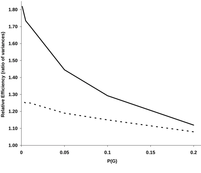
We compare RE for the unmatched versus the matched strategies for specific situations to illustrate the potential improvement in efficiency from the unconditional analysis approach. Figure 1 presents RE(U) and RE(C) for different frequencies of G for a dominant gene with RG=3,

RE=2, RI=5, P(E)=0.2, and F=0.5. The results show a dramatic effect of P(G) on RE for both

analyses. RE(U) decreases from 1.82 at P(G)=0.001 to 1.12 when P(G)=0.2. The slope for RE(C) is

less steep as RE(C) decreases from 1.26 to 1.08 when P(G) increases from 0.001 to 0.2. Figure 1

also illustrates a more pronounced improvement in power for the unconditional analysis relative to the conditional analysis when P(G) is rare. For example, U/C=1.44 when P(G) = 0.001 (and 1.36 when P(G) = 0.01) versus 1.12 when P(G) = 0.1 (and 1.04 when P(G)=0.2).

The gain and/or change in RE(U) and U/C is insignificant for common genes and/or

moderate effect estimates. For example, when P(G)=0.2 and RI=RG=RE=1.5, RE(U)=1.03 and

U/C=1.00. In addition, for moderate effect estimates when P(G) > 0.1, there is little change in RE as P(E) changes and U/C approximates one (i.e. 1.00-1.02) (data not shown).

(8)

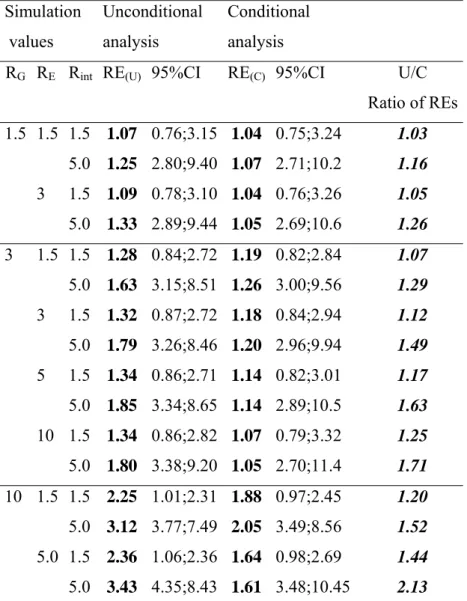
(Table 3 here) Table 3 compares RE(U) and RE(C) for different RG, RE and RI effects when

P(G)=0.01, P(E)=0.2, and F=0.5. The results show that RG and RI have the strongest effect on

RE(U) and that RE(U) increases substantially as either RG or RI increases. An increase in RE leads

to a minor increase in RE(U). In contrast, RE and RI have almost no effect on RE(C); only an

increase in RG leads to any observable increase in RE(C). Thus, U/C ranges from 1.03 for

moderate effects (RI=RG=RE=1.5) to 2.13 for very strong effects (RG=10, RI=RE=5). Indeed,

there is generally about a 50% improvement in power for the unconditional analysis compared to the conditional analysis with high or very high estimates of RG, RI or even RE. Also, as

previously mentioned, when P(G) is common, there is little increase in U/C as RE, RG, or RI

increase from moderate (1.5) to high (5.0) values (data not shown).

Table 3 also presents the 95% confidence intervals for RI. The lower and upper bounds

for the unconditional analysis are contained within the bounds for the conditional analysis illustrating the improved efficiency for the unconditional analysis. This comparison also serves as a check on the validity of the required assumptions for the unconditional analysis. For example, when there is a correlation in E between siblings (ORec≠1), thus violating one of the

required assumptions, the confidence bounds for RI from the unconditional analysis is no longer

contained within the bounds from the conditional analysis. To illustrate this situation, consider a model with P(G)=0.01, P(E)=0.2, RE=1.5, RG=3 and RI=5, and a moderate correlation in E

between siblings, i.e. ORec=2. Under this scenario, the estimates of P(E) among the related and

unrelated controls differ by 7.7% and yield biased estimates of RE, RI, and RG for the

unconditional analysis. This produces 95% confidence intervals of RI that are no longer nested

(i.e., 95% CI from conditional analysis: 2.89, 9.41; 95% CI from unconditional analysis: 2.55, 6.54). In addition, as ORec increases, the bias in RE and RI increase (data not shown). Finally,

table 3 shows that, as expected, as U/C increases, the confidence interval for the unconditional analysis becomes narrower relative to the confidence interval for the conditional analysis.

Incorporation of family-specific baseline risks (represented by H) had no effect on RI for

either the conditional or unconditional analysis (data not shown). This finding was as expected since H was not associated with either G or E. If there had been a correlation with E, for example, the results would have been comparable to that observed when ORec≠1 since P(E)

would not have been equal in the two control groups. Specifically, the unconditional analysis would not be valid and estimates of RE, RI, and RG would all be biased.

(9)

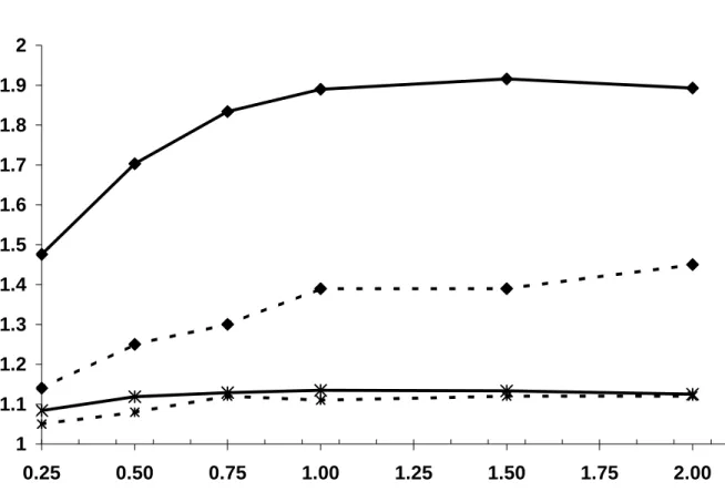
Figure 2 presents RE(U) and RE(C) for different values of F for a rare (P(G)=0.01) and a

common (P(G)=0.2) dominant gene. F varies from 0% to 200% resulting in 0 to 2 sibling controls per case. All other parameters are fixed with P(E)=0.2, RE=2, RG=3, RI=5. The results

show a similar effect of F on RE for both analyses. When P(G)=0.01, there is a substantial increase in RE from F=0.25 to F=1.0 followed by a plateau. The magnitude of the RE is much greater for RE(U) compared to RE(C) and U/C varies from 1.3 to 1.5 with a mean improvement for

the unconditional analysis of 40%. In contrast, when the gene is common (P(G)=0.2), there is a negligible change in RE as F increases and there is essentially no difference between the unconditional and conditional analyses, i.e., U/C varies from 1.0 to 1.04.

Discussion

We have shown that unconditional logistic regression analysis of data from a case-combined-control study to detect GxE interaction is often more efficient than a conditional analysis, particularly for a rare gene and strong effects. The unconditional analysis is also at least as efficient as the conditional analysis when the gene is common and the main and joint effects of E and G are small. Naturally, under the required assumptions, the unconditional analysis retains more data information than does the conditional analysis for which only discordant case-control pairs are informative leading to more precise estimates of the odds ratios7_.

The gain in efficiency for detecting a GxE interaction using unconditional analysis may have a non- negligible effect on the feasibility of a study, i.e. on the required sample size. We previously illustrated1 several feasible scenarios with 80% power involving a rare gene that required about 1000 cases: 1500 controls when a conditional analysis was used. Performing an unconditional analysis at the same power (80%) would only require approximately 750 cases, leading to a total decrease in study subjects of about 625 (250 cases, 250 unrelated and about 125 related controls). Obviously, for situations that require many more subjects (e.g. >20 000 cases and 30 000 controls), even the substantial increase in efficiency associated with the unconditional analysis will not lead to reasonable sample sizes.

As we previously discussed1_{, the major assumptions (e.g. no population stratification bias}

for the unrelated controls and no difference in the distribution of variables of interest between cases who have sibling-controls versus those cases without such sibling-controls plus exchangeability of covariates of interest in cases and sibling controls4,5,8-10 ) required for the

(10)

case-combined-control study to produce valid estimates of main and/or interaction effects are not testable before the data has been collected. If these major assumptions are not met, then alternative analytic strategies will be required. However, if these assumptions are met, then conducting conditional and/or unconditional analyses will depend on the goals of the study and a second set of assumptions. Specifically, for conditional analyses to estimate both main and interaction effects, we require that there is homogeneity between the odds ratios of the variables involved in the GxE interactions using either of the two types of controls. Additionally, for the unconditional analyses to be valid there must be no correlation in E between siblings and the same frequency of E in the two control groups. Although P(E)rel = P(E)unr leads to

unr E rel

E OR

OR = and rel unr

OR

OR_int = _int as long as G and E are independent and the other required assumptions are met, in real settings, these relationships may be more complicated. Specifically, because of confounding, effect modification, etc., the equality of the frequency of E in the two control groups may not necessarily translate to equivalency of the effect estimates. Therefore, the necessary assumptions for the validity of the unconditional analysis should also include the

equality unr

E rel

E OR

OR = . For purposes of this study, we implicitly assumed that there was no correlation within families due to shared, but unmeasured factors. Examination of H with different risks across families showed that if H was not correlated with E or G, it had no effect on RI or its variance and thus no effect on the relative efficiency. However, if H was correlated with

E, it would be comparable to having a correlation in E between siblings with different values across families leading to different frequencies of E between control groups and therefore invalid estimates for the E main effect as well as the GxE interaction effect under an unconditional analysis.

Under the assumptions listed above and detailed in the methods, unconditional analysis of data from the case-combined-control study yields unbiased estimates of the E main effect and GxE interaction effect. The conditional analysis, however, can serve as a check on the validity of the unconditional analysis strategy by evaluation of the confidence intervals for the GxE interaction effect estimate RI. Specifically, if the unmatched approach is valid, given the

increased efficiency for an unconditional versus a conditional analysis, the lower and upper bounds for the RI confidence interval from the unconditional analysis should be contained within

the confidence interval for the conditional analysis. If the confidence interval bounds for the

(11)

unconditional analysis are not within the bounds for the conditional analysis, then one may expect that one or more of the required assumptions is not valid. However, there may be situations when the deviation from the required assumptions (e.g. existence of a correlation in E between siblings) may be small such that unconditional analysis could still be conducted without much bias. Further study is required to determine how robust RE andRI are to small or moderate

deviation from these assumptions. Moreover, it may be helpful to consider the types of scenarios when the required assumptions would be likely to apply. Depending on the disease and exposures of interest, external data may be available to provide a priori information about, for example, the chances of a correlation in exposure E between siblings. If such a correlation is known or strongly suspected, unconditional analysis would not be appropriate and a different analytic strategy would be required.

If the necessary assumptions for the conditional or unconditional analysis of the case-combined-control design are not met, then one may choose an alternative analytical strategy such as polytomous regression or incorporation of weights to account for the differential ascertainment of the two control groups. Another possible approach would be to combine the conditional and unconditional logistic regressions in a single analysis. That is, one could use a conditional likelihood for the sibling controls and a full likelihood for the unrelated controls and maximize the product of the likelihoods. Limited simulations using such an approach suggest that this analytical strategy is substantially less efficient than the unconditional analysis but appears generally as efficient as the conditional analysis (data not shown). An advantage of this approach, however, is that it appears to produce minimally biased estimates of RG and RE even

when there is a correlation in E between siblings. Since this approach may require fewer assumptions than either unconditional or conditional analysis strategies, the efficiency reductions might be offset by improved estimation capabilities. Further evaluation of this strategy and other analytical approaches are planned. If one is interested in estimating the main effect of G, then unconditional analysis cannot be conducted. Also, since validity of the unconditional analyses requires the same frequency for at least one variable in the interaction for both control groups, it follows that unconditional analysis cannot be used to estimate GxG interaction effects. The unconditional analysis approach is limited to GxE interactions or ExE interactions so long as at least one of the exposure variables is not correlated among siblings and has the same frequency in the two control groups.

(12)

The case-combined-control design was developed to increase efficiency for GxE interaction detection by simultaneously using two types of controls. Other designs such as the case-control-family design11_{and the triads [affected offspring plus two parents] and unrelated}

subjects design12, 13 with simultaneous use of multiple control groups have also been proposed. As molecular genetic data becomes more easily collected and less expensive, there will be increased opportunities for these types of hybrid designs to increase power for detection of genetic or environmental main effects and interaction effects.

These results show that unconditional analysis of the case-combined-control design to estimate GxE interaction is unbiased under certain conditions and may produce a substantial increase in power. However, necessary assumptions for such an analysis may not be met for all variables of interest. Future studies will examine whether the case-combined-control design would still offer advantages over a single case-unrelated-control or case-related-control study design in these situations.

Grants and Acknowledgements

This project was supported in part by INSERM, the Foundation Philippe INC, the Association pour la Recherche contre le Cancer and the University of Paris Sud. This work was supported in part by the Intramural Research Program of the National Institutes of Health, National Cancer Institute, Division of Cancer Epidemiology and Genetics. This work was initiated while Nadine Andrieu was a guest researcher at the Genetic Epidemiology Branch of the National Cancer Institute. The authors thank Angela Fahey, IMS for her assistance with the simulations, Dr. John Thompson (University of Leicester, UK) for analytic support and the reviewers for helpful comments

(13)

Appendix Cases Controls related unrelated E- G- a c e G+ b d f E+ G- g i k G+ h j l

The above table shows the E and G distributions for cases, related, and unrelated controls. If one is interested in using the case-combined-control design approach to estimate main and interaction effects, then the approach requires that there is homogeneity between the odds ratios of the variables involved in the GxE interactions using either of the two types of controls1. That is, the ORs for G and E for the two control groups are required to be equal. For this assumption to be valid, a matched analytic strategy is required since siblings will have a greater frequency of G (and also E if there is a positive correlation in E between cases and their sibling controls) compared to unrelated controls.

However, if one is mainly interested in estimating the GxE interaction effect, then only

the equality rel unr

OR

OR_int = _int is required where rel denotes related and unr, unrelated controls. Thus, from the above table

af be ak gela he ad bc ai gc ja hc OR OR OR OR OR OR unr G unr E unr G , E rel G rel E rel G , E ₌ _⇒ ₌ thus le kf jc id OR

OR_intrel = _intunr ⇒ =

For this equality to hold, we assume that G and E are independent. In addition, since G is correlated in siblings, we also require no correlation in E between siblings which means that P(E)rel = P(E)unr. Given these requirements, from the above table, we have i/c=k/e and j/d=l/f.

(14)

Thus, unr E rel

E OR

OR = in addition to rel unr

OR

OR_int = _int and an unconditional analysis may be performed in the case-combined-control design to estimate the GxE interaction effect. Both the GxE interaction effect and E main effect estimates are unbiased. If, however, there is a correlation in E between siblings and/or P(E)rel ≠ P(E)unr, then i/c≠k/e and j/d≠l/f. And it follows that ORrel_E ≠ORunr_E and rel unr

OR

ORint ≠ int . Under such a scenario, unconditional analysis of case-combined-control data would not be valid.

References

1_{Andrieu N, Goldstein AM. The case-combined-control design was efficient in detecting}

gene-environment interactions. J Clin Epidemiol 2004;57:662-71.

2_{Andrieu N, Demenais F. Interactions between genetic and reproductive factors in breast cancer}

risk in a French family sample. Am J Hum Genet 1997;61:678-90.

3_{Botto LD, Khoury MJ. Commentary: facing the challenge of gene-environment interaction: the}

two-by-four table and beyond. Am J Epidemiol 2001;153:1016-20.

4_{Langholz B, Ziogas A, Thomas DC et al. Ascertainment bias in rate ratio estimation from}

case-sibling control studies of variable age-at-onset diseases. Biometrics 1999;55:1129-36.

5_{Siegmund KD, Langholz B. Ascertainment bias in family-based case-control studies. Am J}

Epidemiol 2002;155:875-80.

6_{Stata Corp. Stata statistical software: Release 7.0. College station, Tx: Stata corporation. 2001.} 7_{Rothman KJ, Greenland S. Modern Epidemiology, second edition. Lippincott-Raven,}

Philadelphia 1998.

8_{Wacholder S, Rothman N, Caporaso N. Population stratification in epidemiologic studies of}

common genetic variants and cancer: quantification of bias. J Natl Cancer Inst 2000;92:1151-8.

(15)

9_{Caporaso N, Rothman N, Wacholder S. Case-control studies of common alleles and}

environmental factors. J Natl Cancer Inst Monogr 1999;26:25-30.

10_{Millikan RC. Re: Population stratification in epidemiologic studies of common genetic variants}

and cancer: quantification of bias. J Natl Cancer Inst 2001;93:156-8.

11_{Hopper JL, Chenevix-Trench G, Jolley DJ et al. Design and analysis issues in a}

population-based, case-control-family study of the genetic epidemiology of breast cancer and the co-operative family registry for breast cancer studies (CFRBCS). J Natl Cancer Inst Monogr 1999;26:95-100

12_{Nagelkerke NJD, Hoebee B, Teunis P, Kimman TG. Combining the transmission}

disequilibrium test and case-control methodology using generalized logistic regression. Eur J Hum Genet 2004;12:964-70.

13_{Epstein MP, Veal CD, Trembath RC et al. Genetic association analysis using data from triads}

and unrelated subjects. Am J Hum Genet 2005;76:592-608.

(16)

Table 1: Definition of parameters for modelling GxE interaction

Symbols Definition

F Average number of available controls per case p Population frequency of the “mutant” allele A PG =P(G) Prevalence of the genetic factor G in the population.

(equal to p²+2p(1-p) under a dominant model and equal to p² under a recessive model)

PE =P(E) Prevalence of the environmental factor E in the population RE Odds ratio between E and disease (among those not having G) RG Odds ratio between G and disease (among those not exposed to E)

RI Interaction effect, defined on a multiplicative scale.

(17)

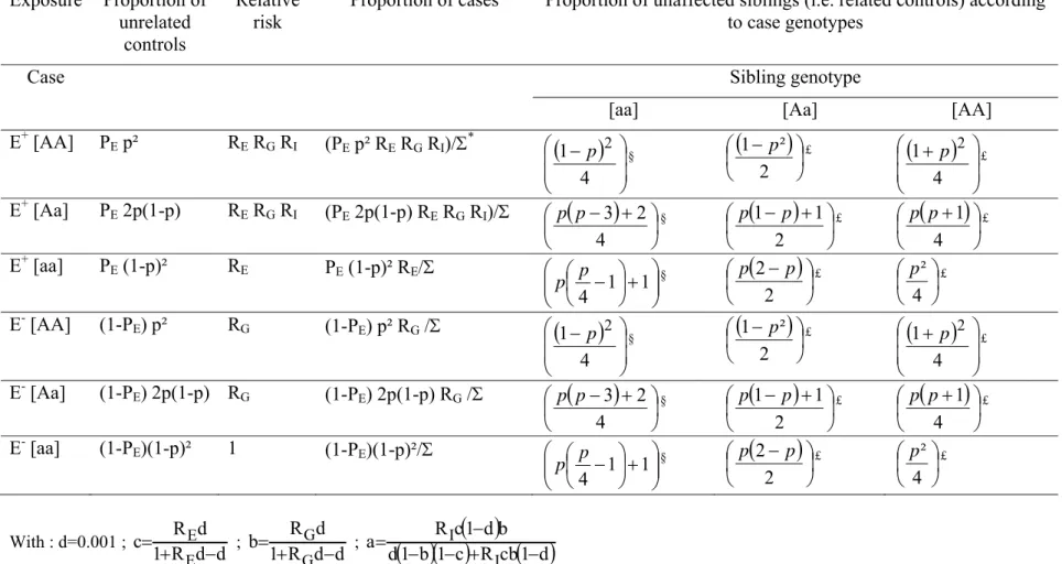
Table 2: Subgroups of the population at different risk of disease when there is a GxE interaction, where A is an autosomal dominant allele1 Exposure Proportion of unrelated controls Relative risk

Proportion of cases Proportion of unaffected siblings (i.e. related controls) according to case genotypes

Case Sibling genotype

( )

_{( )}

d 1 cb R c 1 b 1 d b d 1 c R a I I − + − − − = * Σ=PE (p²+2p(1-p) RE RG RI + PE (1-p)² RE + (1-PE)(p²+2p(1-p) RG + (1-PE)(1-p)² § _{multiply by (1-b)(1-P}

E) when sib control not exposed to E, and by (1-a)PE when sib control exposed to E £_{multiply by (1-d)(1-P}

E) when sib control not exposed to E, and by (1-c)PE when sib control exposed to E

(18)

Table 3: Comparison of the relative efficiency using either unconditional analysis or conditional analysis for different G, E and GxE effects for P(G)=0.01; P(E)=0.2

Simulation values Unconditional analysis Conditional analysis

RG RE Rint RE(U) 95%CI RE(C) 95%CI U/C

Ratio of REs 1.5 1.5 1.5 1.07 0.76;3.15 1.04 0.75;3.24 1.03 5.0 1.25 2.80;9.40 1.07 2.71;10.2 1.16 3 1.5 1.09 0.78;3.10 1.04 0.76;3.26 1.05 5.0 1.33 2.89;9.44 1.05 2.69;10.6 1.26 3 1.5 1.5 1.28 0.84;2.72 1.19 0.82;2.84 1.07 5.0 1.63 3.15;8.51 1.26 3.00;9.56 1.29 3 1.5 1.32 0.87;2.72 1.18 0.84;2.94 1.12 5.0 1.79 3.26;8.46 1.20 2.96;9.94 1.49 5 1.5 1.34 0.86;2.71 1.14 0.82;3.01 1.17 5.0 1.85 3.34;8.65 1.14 2.89;10.5 1.63 10 1.5 1.34 0.86;2.82 1.07 0.79;3.32 1.25 5.0 1.80 3.38;9.20 1.05 2.70;11.4 1.71 10 1.5 1.5 2.25 1.01;2.31 1.88 0.97;2.45 1.20 5.0 3.12 3.77;7.49 2.05 3.49;8.56 1.52 5.0 1.5 2.36 1.06;2.36 1.64 0.98;2.69 1.44 5.0 3.43 4.35;8.43 1.61 3.48;10.45 2.13

(19)

Figure 1: Relative efficiency from unconditional analysis, RE(U) (bold-line) and from

conditional analysis RE(C) (dashed-line) according to the frequency of G for a dominant gene

with RG=3, RE=2, RI=5, P(E)=0.2, and F=0.5.

1.00 1.10 1.20 1.30 1.40 1.50 1.60 1.70 1.80 0 0.05 0.1 0.15 0.2 P(G) R e lati v e E fficiency (ratio of vari a nc es)

(20)

Figure 2: Relative efficiency from unconditional analysis, RE(U) (bold-line) and from

conditional analysis RE(C) (dashed-line) according to the number of available sibling controls per

case for a rare (P(G)=0.01: diamond-symbols) and common (P(G)=0.2: stared-symbols) dominant gene with P(E)=0.2; RE=2; RG=3; RI=5.

1 1.1 1.2 1.3 1.4 1.5 1.6 1.7 1.8 1.9 2 0.25 0.50 0.75 1.00 1.25 1.50 1.75 2.00