Stochastic vehicle routing : from theory to practice

(1)

From Theory to Practice

Doctoral Dissertation submitted to the

Faculty of Informatics of the Università della Svizzera Italiana in partial fulfillment of the requirements for the degree of

Doctor of Philosophy

presented by

Dennis Weyland

under the supervision of

Luca Maria Gambardella and Roberto Montemanni

(2)

(3)

Evanthia Papadopoulou Università della Svizzera Italiana, Switzerland

Fabian Kuhn Università della Svizzera Italiana, Switzerland

Richard Hartl University of Vienna, Austria

Arne Løkketangen Molde University College, Norway

Dissertation accepted on 29 July 2013

Research Advisor Co-Advisor

Luca Maria Gambardella Roberto Montemanni

PhD Program Director

Antonio Carzaniga

(4)

mitted previously, in whole or in part, to qualify for any other academic award; and the content of the thesis is the result of work which has been carried out since the official commencement date of the approved research program.

Dennis Weyland Lugano, 29 July 2013

(5)

(6)

(7)

Abstract

In this thesis we discuss practical and theoretical aspects of various stochastic vehicle routing problems. These are combinatorial optimization problems re-lated to the field of transportation and logistics in which input data is (partially) represented in a stochastic way. More in detail, we focus on two-stage stochastic

vehicle routing problemsand in particular on so-called a priori optimization

prob-lems. The results are divided into a theoretical part and a practical part. In fact, the theoretical results provide a strong motivation for the development and the usage of the methods presented in the practical part.

We begin the theoretical part with a convergence result regarding vehicle routing problems with stochastic demands. This result can be used to give ex-planations for some phenomena related to these problems which have been re-ported in literature. We then continue with hardness results for stochastic vehi-cle routing problems on substantially stochastic instances. Here we show that several stochastic vehicle routing problems remain NP-hard even if they are re-stricted to instances which differ significantly from non-stochastic instances. Ad-ditionally, we give some inapproximability results for these problems restricted to substantially stochastic instances. After that, we focus on a stochastic vehi-cle routing problem which considers time dependencies in terms of deadlines. We show that various computational tasks related to this problem, including the evaluation of the objective function, are #P-hard even for Euclidean instances. Note that this is a very strong hardness result and it immediately implies that these computational tasks are also NP-hard. We then further investigate the objective function of this problem. Here we demonstrate that the existing ap-proximations for this objective function are not able to guarantee any reasonable worst-case approximation ratio. Finally, we show that it is NP-hard to approxi-mate the objective function of a slightly more general problem within any rea-sonable worst-case approximation ratio.

In the practical part we develop and apply various methods for the opti-mization of stochastic vehicle routing problems. Since the theoretical results indicate that it is a great challenge to optimize these problems, we focus mainly

(8)

on heuristic methods. We start with the development of strong local search al-gorithms for one of the most extensively studied stochastic vehicle routing prob-lems. These algorithms use an efficient approximation of the objective func-tion based on Monte Carlo sampling. They are then further used within dif-ferent heuristics, leading to new state-of-the-art methods for this problem. We then transfer our results to a more intricate stochastic vehicle routing problem. Here we first present an approximation of the objective function using the novel method of quasi-parallel evaluation of samples. Then we again develop strong local search algorithms and use them within more complex heuristics to obtain new state-of-the-art methods. After that we change the scope towards a general framework for the optimization of stochastic vehicle routing problems based on general purpose computing on graphics processing units. Here we are exploiting the massive computational power for parallel computations offered by modern graphics processing units in the context of stochastic vehicle routing problems. More in detail, we propose to use an approximation of the objective function based on Monte Carlo sampling which can be parallelized in an extremely effi-cient way. The effectiveness of this framework is then demonstrated in a case study. We finish the practical part with an application of our methods to a real world stochastic vehicle routing problem. This problem is part of a project that has been initiated in 2010 by Caritas Suisse. It is still in an early stage, but with our work we were able to successfully support some of the decision processes at this stage.

(9)

Acknowledgements

At this point I want to thank everyone who helped me in the last years to make this document possible. Shame on me for those people that I forgot to mention. First of all, let me give credits to my parents Ernst-Albert and Maria Weyland and to my sister Julia Weyland. You have constantly supported me for my whole life and there are no words that could acknowledge your endless efforts in a proper way. At the end it is you who made the largest contribution to this docu-ment. Thank you for all your care and for affording me the education I got: at home, at school, and at university.

Then I want to acknowledge the support and help from my research advisor

Luca Maria Gambardella, my co-advisor Roberto Montemanni and also my for-mer supervisor Leonora Bianchi, all from the Dalle Molle Institute for Artificial Intelligence (IDSIA), Switzerland. Your efforts and encouragements helped me to arrive at this point.

Let me continue to thank my dissertation committee (in alphabetic order):

Richard Hartlfrom the University of Vienna, Austria, Fabian Kuhn from the Uni-versità della Svizzera Italiana (USI), Switzerland, Arne Løkketangen from the Molde University College, Norway, and Evanthia Papadopoulou from the Univer-sità della Svizzera Italiana (USI), Switzerland.

Many thanks are given to the different PhD Program Directors at the Univer-sità della Svizzera Italiana (USI), Switzerland, during the last years (in alpha-betic order): Antonio Carzaniga, Fabio Crestani, and Michele Lanza.

Let me also thank all my colleagues at the Dalle Molle Institute for Artificial Intelligence (IDSIA), Switzerland, the Scuola Universitaria Professionale della Svizzera Italiana (SUPSI), Switzerland, and the Università della Svizzera Italiana (USI), Switzerland. I had a great time with you guys and you provided me a very nice working environment.

At this point I have to apologize to a very special person in my life, Michela

Papandrea. I am sorry for all the time I could not spend with you while I was working on this document. Thanks a lot for your patience, your support and your love.

(10)

Finally, I would like to give thanks to some persons that contributed to my research in one way or another (again in alphabetic order): David Adjiashvili,

Reinhard Bürgy, Cassio de Campos, Dan Ciresan, Patrick Czaplicki, Peter Detzner,

Andrei Duma, Michael Felten, Alexander and Anna Förster, Kail Frank, Fred Glover,

Jan Hofeditz, Jan Koutnik, Juxi Leitner, Jonathan Masci, Ueli Meier, Nikos

Mut-sanas, David Pritchard, Rudolf Scharlau, Kaspar Schüpbach, Georgios Stamoulis,

(11)

Chapter 1 Introduction

In this introductory chapter we provide the basic knowledge and the background information that are required in the remaining part of this thesis. We first put our research work into a broader context. We start with a discussion of

opti-mization under uncertainty(Diwekar[2008]) and then we gradually confine the classification of our work within the fields of stochastic combinatorial

optimiza-tion(Bianchi et al.[2009]), stochastic vehicle routing (Gendreau et al. [1996a]),

two-stage stochastic combinatorial optimization(Schultz et al.[2008]) and finally

a priori optimization (Bertsimas et al. [1990]). We continue with a discussion of four stochastic vehicle routing problems that are used throughout the thesis. We motivate these problems, we present related literature and we give formal definitions. After that we finish the introductory part with a brief outlook on the following chapters.

1.1 Classification of the Research Area

In the last decades optimization under uncertainty (Diwekar [2008]; Sahini-dis [2004]; Freund [2004]; Gutjahr [2004]) has received increasing attention. This field deals with combinatorial optimization problems that consider uncer-tainty of the given information directly in the problem definition. In this way real world problems can be modeled in a more realistic way. Since we are confronted with uncertain information in many aspects of our lives, it is not surprising that optimization under uncertainty has plenty of applications in nu-merous areas. Among them are for example the generation of electrical power (Dentcheva and Römisch [1998]; Nowak and Römisch [2000]), the operation of water reservoirs (Cervellera et al. [2006]; Karamouz and Vasiliadis [1992]; Stedinger et al. [1984]), applications related to inventory management

(14)

teus[1990]; Hvattum et al. [2009]; You and Grossmann [2008]; Zheng [1992]; Hariga and Ben-Daya[1999]), portfolio selection (Samuelson [1969]; Inuiguchi and Ramık [2000]; Zhou and Li [2000]; Liu [1999]), facility planning (Chen et al. [2006]; Ermoliev and Leonardi [1982]; Louveaux and Peeters [1992]; Chang et al. [2007]), pollution control (Wong and Somes [1995]; Adar and Griffin[1976]; Horan [2001]), stabilization of mechanisms (Wang et al. [2002, 2010]; Lu et al. [2009]), analysis of biological systems (Frank et al. [2003]; Isukapalli et al.[1998]; Wilkinson [2009]), network design problems (Hoff et al. [2010]), scheduling problems (Almeder and Hartl [2012]) and applications in the field of transportation and logistics (Powell and Topaloglu[2003]; Shu et al. [2005]; Cooper and Leblanc [1977]; Barbarosoˇglu and Arda [2004]). While on the one hand such problems based on more realistic models can be used to obtain more meaningful results, these problems are on the other hand usually much harder to solve than the non-stochastic counterparts. Therefore, it is of great importance to develop efficient methods for solving such problems.

There exist different ways in which the uncertainty can be modeled. One possibility is to provide possible values for the input data instead of only a sin-gle value, for example in terms of intervals. It is assumed that the real data is among these values, but no further knowledge about the likelihood of the different values is given. This leads to the field of robust optimization (Ben-Tal and Nemirovski[2002]; Beyer and Sendhoff [2007]; Ben-Tal et al. [2009]). Here the task is to find solutions with a certain robustness against the uncer-tainty. Another possibility is to use fuzzy variables to express unceruncer-tainty. Prob-lems using such fuzzy variables for the input belong to the field of fuzzy

opti-mization (Negoita and Ralescu[1977]; Delgado et al. [1994]; Luhandjula and Gupta [1996]). One different possibility is to represent the uncertainty using stochastic data, for example by means of probability distributions. This field is called stochastic combinatorial optimization (Gutjahr [2003]; Hentenryck and Bent [2009]; Immorlica et al. [2004]; Carraway et al. [1989]; Bianchi et al. [2009]). By using probability distributions, we somehow specify possible values for the different input data, like also for robust optimization. Here the main dif-ference is that we additionally assume to have knowledge about the likelihood of these different values. In most of the cases the optimization goal is then to optimize a certain stochastic value, for example the expected costs of a solution, with respect to the given probability distributions.

In this thesis we focus on stochastic combinatorial optimization problems. More in detail, we focus on stochastic vehicle routing problems (Gendreau et al. [1996a]; Stewart and Golden [1983]; Hemmelmayr et al. [2009]; Dror and Trudeau[1986]; Kenyon and Morton [2003]; Yang et al. [2000]; Bertsimas et al.

(15)

[1995]; Gendreau et al. [1996b]; Bertsimas [1992]; Bastian and Rinnooy Kan [1992]; Gendreau et al. [1995]; Hvattum et al. [2006]; Secomandi [2001]; Liu and Lai [2004]; Schilde et al. [2011]). These are stochastic combinatorial

opti-mization problems arising in the field of transportation and logistics. While in general uncertainty can be modeled in many different ways, in the field of trans-portation and logistics it is reasonable to model the uncertainty of several aspects in a stochastic way. For example, probability distributions for travel times, for customers’ demands and for the presence of customers can be obtained based on historical data.

Many such stochastic vehicle routing problems are modeled as so called

two-stage stochastic combinatorial optimization problems(Schultz et al.[2008]; Carøe and Tind [1998]; Klein Haneveld and van der Vlerk [1999]; Dhamdhere et al. [2005]; Uryasev and Pardalos [2001]). Here the idea is to make an initial de-cision at the first stage, where the stochastic information is available without knowing the actual realizations of the stochastic events. After the realizations of the stochastic events become known, a second stage decision is taken. This deci-sion is based on the first stage decideci-sion and on the realizations of the stochastic events. This framework incorporates many different settings. One extreme case is to omit the first stage completely and to perform the actual optimization just after the realizations of the stochastic events become known. Such an approach is called a reoptimization approach (Secomandi and Margot [2009]; Wu et al. [2002]; Böckenhauer et al. [2008]; Delage [2010]). Although the results of this approach are usually of very high quality, it cannot be applied in a lot of situations. The main problem is that this approach requires certain computa-tional resources, in particular computacomputa-tional time, which is usually not available between the realizations of the stochastic events become known and the final decision has to be taken. The other problem is that for some problems the ac-tual realizations of the stochastic events are gradually revealed. While it is still possible to model such a problem as a two-stage stochastic combinatorial

opti-mization problem, a reoptimization approach cannot be applied here. The other extreme case is to shift the main decision process to the first stage and to use the second stage decision only as a mechanism to assure feasibility of solutions. Since the actual optimization is performed before the realizations of the random events are revealed, this approach is called a priori optimization (Bertsimas et al. [1990]; Laporte et al. [1994]; Murat and Paschos [2002]; Miller-Hooks and Mahmassani[2003]; Campbell and Thomas [2008a]). The quality of solutions computed by an a priori optimization approach are usually worse compared to a reoptimization approach. Nonetheless, in many settings the constraints on the computational resources for the second stage, in particular computation time,

(16)

make an a priori optimization approach necessary. And as we will see later in this section, there are also other reasons why such an approach might be used. In between these two extreme cases other approaches, weighting the first stage and the second stage in different ways, can be found (Birge and Louveaux [1988]; Barbarosoˇglu and Arda [2004]; Huang and Loucks [2000]; Cheung and Chen [1998]).

In this work we focus on a priori optimization. Although the quality of the final solutions is usually better using a reoptimization approach, an a priori

op-timization approach is the method of choice in many different situations. In the context of stochastic vehicle routing there are three main reasons that are in favor of an a priori optimization approach. The first one is that the second stage decision requires only a minimum of computational resources. If every day a new solution is required, the computational resources and in particular the computational time are usually a limiting factor. The second reason is that in some situations the realizations of the stochastic events are not revealed at once, but only step by step. Still these problems can be modeled as a two-stage

stochastic combinatorial optimization problems, but it is not possible to apply a

reoptimization approach. An example here is the collection of waste (Nuortio et al. [2006]; Maqsood and Huang [2003]). Although it is possible to retrieve probability distributions for the amount of waste that has to be collected, the real amount is only revealed during the collection process. Therefore, it is not possible to apply a reoptimization approach, while a proper a priori optimization approach can be used. The last reason holds especially for the class of stochastic

vehicle routing problems. In fact, in the context of stochastic vehicle routing

prob-lems it is very convenient for the customers to be served periodically at roughly the same time. Additionally, it is convenient for the drivers of the vehicles to follow roughly the same route every time. Obviously, a reoptimization approach cannot guarantee these properties in general. On the other hand, many a priori

optimization approaches maintain this property in a natural way. All in all, a

priori optimizationis the method of choice in many different situations. The us-age of a priori optimization is very well motivated and has numerous real world applications.

(17)

1.2 The Main Optimization Problems

used in this Thesis

In this section we discuss those stochastic vehicle routing problems that are the main subjects of investigation in this thesis. Since these problems are used throughout the thesis we decided to examine them already at this point. For all of the four problems presented in this section we give a motivation, we discuss related literature and we present a formal definition. To maintain consistency we refer to these problems with the names commonly used in literature. We begin with the well studied PROBABILISTIC TRAVELING SALESMAN PROBLEM (Jail-let[1985]; Laporte et al. [1994]; Bianchi et al. [2002a]; Bertsimas and Howell [1993]). This problem is a generalization of the famous TRAVELING SALESMAN PROBLEM (Lawler et al. [1985]; Lin [1965]; Held and Karp [1970]; Johnson and McGeoch [1997]) where in addition the presence of customers is modeled in a stochastic way. After that we discuss the PROBABILISTIC TRAVELING SALES -MANPROBLEM WITH DEADLINES(Campbell and Thomas[2008b, 2009]; Weyland et al. [2012a,b,d,c]) which is a generalization of the PROBABILISTIC TRAVELING SALESMAN PROBLEMconsidering time dependencies in terms of deadlines. Then we examine the VEHICLE ROUTING PROBLEM WITH STOCHASTIC DEMANDS (Bertsi-mas[1992]; Bianchi et al. [2006]; Dror et al. [1993]; Bastian and Rinnooy Kan [1992]). Here the demands of the customers are modeled in a stochastic way and a single vehicle with an integral capacity is used to satisfy the customers’ demands. Finally, we present the VEHICLE ROUTING PROBLEM WITH STOCHASTIC DEMANDS AND CUSTOMERS (Gendreau et al. [1995, 1996b]). This problem is a combination of the PROBABILISTICTRAVELINGSALESMANPROBLEMand the VEHICLE ROUTINGPROBLEM WITHSTOCHASTIC DEMANDS.

1.2.1 The Probabilistic Traveling Salesman Problem

The PROBABILISTIC TRAVELINGSALESMANPROBLEM(PTSP) has been introduced in Jaillet [1985] and is a generalization of the famous TRAVELINGSALESMANPROB -LEM (TSP). Like for the TSP, a set of customers and distances between these customers are given. In addition, the presence of the customers is modeled in a stochastic way. Each customer has assigned a value which represents the proba-bility with which this customer is present. Furthermore, the presence of different customers are independent events. This problem belongs to the class of a priori

optimization problems. Here a solution is a tour visiting all customers exactly once, just as for the TSP. In this context such a solution is called a priori solution

(18)

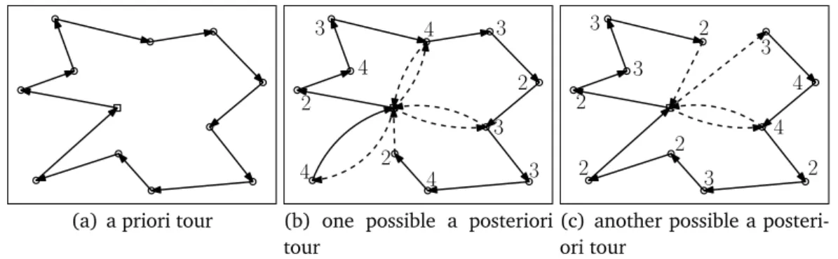
(a) a priori tour (b) one possible a posteriori tour

(c) another possible a posteri-ori tour

Figure 1.1. Example of how a posteriori tours are derived from a given a priori tour for the PTSP. Part (a) shows the given a priori tour. Parts (b) and (c) represent two particular realizations of the random events. Here the filled circles represent the customers that require a visit. These customers are visited in the order specified by the a priori tour, while the other customers are just skipped.

or a priori tour. This reflects that the order of the customers is determined before it is known which customers are present. After the presence of the customers becomes known, a so called a posteriori tour is derived from the a posteriori solution by skipping the customers which are not present. In this way the cus-tomers which are present are visited in the order given by the a priori tour. This process is illustrated in figure 1.1. Now the optimization goal is to find an a priori tour of minimum expected length over the a posteriori tours with respect to the given probabilities.

Most of the literature for the PTSP deals with heuristics for this problem. To our knowledge the only work which proposes an exact method is Laporte et al. [1994]. Here a formulation of the PTSP as an integer stochastic program is introduced. A branch-and-cut algorithm is then used to solve instances of up to 50 customers to optimality. This work was published almost 20 years ago. Although the computational power has increased a lot during the last two decades, the size of the instances which can be solved to optimality has not been significantly improved. In Bertsimas and Howell [1993] some theoretical properties for the PTSP are presented. Among them are improved bounds and asymptotic relations. This work also contains a comparison between the a priori

optimizationapproach and the reoptimization approach. Additionally, some sim-ple heuristics are analyzed. To tackle the PTSP many different metaheuristics have been proposed. Different ant colony optimization approaches are presented in Bianchi et al.[2002a,b]; Branke and Guntsch [2003]; Gutjahr [2004]; Branke

(19)

and Guntsch[2004]. A hybrid scatter search approach for the PTSP is discussed in Liu [2007] and an improved local search strategy for this approach is given in Liu [2008a]. A heuristic based on the aggregation of customers into clusters is proposed in Campbell[2006]. A memetic algorithm for the PTSP is suggested in Liu [2008b]. The generation of initial solutions is discussed in the context of genetic algorithms in Liu [2010]. In Marinakis et al. [2008]; Marinakis and Marinaki[2009, 2010] the authors present a greedy randomized adaptive search procedure, a hybrid honey bees mating optimization algorithm and a hybrid multi-swarm particle swarm optimization algorithm. Methods based on an ap-proximation of the objective function using Monte Carlo sampling are discussed in Balaprakash et al.[2009b,a, 2010]; Birattari et al. [2008b]. In Birattari et al. [2008b] a local search algorithm using such an approximation of the objec-tive function is proposed. A hybrid ant colony optimization approach based on this local search is then presented in Balaprakash et al. [2009b]. Further im-provements for the local search algorithm are introduced in Balaprakash et al. [2009a] and metaheuristics based on this local search are finally presented in Balaprakash et al.[2010].

Before we give a formal definition of this problem, we would like to present an expression for the costs of an a priori tour. Let V be the set of n customers, let d : V × V → R+ be a function representing the distances between these cus-tomers and let p : V → [0, 1] be a function representing the probabilities of the customers’ presence. Given a permutation τ : 〈n〉 → V of the customers, which represents an a priori tour, the expected costs over the a posteriori tours with respect to the given probabilities can be computed according to Jaillet[1985] as

fptsp(τ) = n X i=1 n X j=i+1

E(cost generated by the edge from τi toτj)

+ n X i=1 i−1 X j=1

E(cost generated by the edge from τi toτj)

= n X i=1 n X j=i+1 d(τ_i,τ_j) p(τ_i) p(τ_j) j−1 Y k=i+1 (1 − p(τk)) + n X i=1 i−1 X j=1 d(τ_i,τj) p(τi) p(τj) n Y k=i+1 (1 − p(τk)) j−1 Y k=1 (1 − p(τk)).

Due to linearity of expectation the expected costs of the a posteriori tours is the sum of the expected costs generated by the edges between any pair of

(20)

customers. The expected cost generated by the edge between two customers is the distance between these customers multiplied by the probability that these customers are next to each other in an a posteriori solution. Customers τi and

τjare next to each other in an a posteriori solution if both customers are present

and if all customers between τ_i andτ_j are not present. Since the indices of the sums and products in the given formula range over at most n values, the costs of an a priori solution can be trivially computed in O (n3_{) arithmetic operations.} Using a specific order for the summations, the computational time can be re-duced toO (n2) (Jaillet [1985]). Using this expression for the costs of an a priori tour, we are now able to define the PTSP formally.

Problem 1 (PROBABILISTICTRAVELINGSALESMANPROBLEM(PTSP)). Given a set V

of size n, a function d : V × V → R+ and a function p: V → [0, 1], the problem

is to compute a permutation τ? : 〈n〉 → V , such that fptsp(τ?) ≤ fptsp(τ) for any

permutationτ : 〈n〉 → V .

1.2.2 The Probabilistic Traveling Salesman Problem

with Deadlines

In Campbell and Thomas[2008b] the PROBABILISTICTRAVELINGSALESMANPROB -LEM WITH DEADLINES (PTSPD) has been introduced as a generalization of the PROBABILISTIC TRAVELINGSALESMANPROBLEMwhere time dependencies are mod-eled in terms of deadlines. More in detail, four different variants were pro-posed: three recourse models and one chance constrained model. In this thesis we will concentrate on the two very similar variants called PTSPD RECOURSE I with fixed penalties and PTSPD RECOURSEI with proportional penalties. We will formally introduce the PTSPD RECOURSE I with fixed penalties and refer to this problem simply as the PROBABILISTIC TRAVELINGSALESMAN PROBLEM WITH DEAD -LINES. Nonetheless, all our results can also be generalized with similar proofs to the other models. As for the PTSP we model the presence of the customers in a stochastic way. Additionally, each customer has assigned a deadline and a penalty value. We are then interested in an a priori solution with minimum expected costs over the a posteriori solutions. For this problem the costs of the a posteriori solutions are the travel times plus penalties for deadlines which are violated. For each violated deadline a fixed penalty, dependent on the customer, incurs. Note that for the variant called PTSPD RECOURSE I with proportional penalties the penalties for missed deadlines are proportional to the delay. This is the only difference to the model with fixed penalties.

(21)

Since the PTSPD has been introduced recently in 2008, not a lot of publi-cations are dealing with this problem so far. In Campbell and Thomas [2008b] the problem is introduced and all the four variants are formally defined. Some theoretical properties are derived and some artificial special cases of the prob-lem are discussed. The only other publication regarding the PTSPD is Campbell and Thomas [2009]. Here approximations for the objective function are intro-duced. These approximations are then compared with the exact evaluation of the objective function using a simple local search algorithm. It has been shown that the approximations can be used within the local search in combination with the exact evaluation of the objective function to obtain solutions of competitive quality, while the computational time could be reduced significantly. Although the computational complexity of the PTSPD objective function was not known, the authors stated that one of the main challenges for the PTSPD is the computa-tionally demanding objective function. We show in this work that the objective function is in fact hard to compute from a computational complexity point of view. Additionally, we also show how to address this challenge and how to ob-tain high quality solutions within a reasonable computational time.

The formal definition of the PTSPD is similar to that of the PTSP. With V we refer to the set of n customers. As for the PTSP we have given distances between the locations which are represented by a function d : V × V → R+and probabilities for the customers’ presence which are represented by a function

p : V → [0, 1]. Since we are using time dependencies, the routes require a fixed starting point. This starting point is a special element v1 ∈ V for which we set p(v1) = 1. In this context the starting point is usually called the depot. The deadlines for the different customers are now modeled using a function

t : V → R+ and the penalty values for the different customers are modeled using a function h : V → R+. To keep the mathematical formulation as simple as possible we also define these values for the depot v₁, although we will meet the deadline at the depot in any case, since we start the tour there. An a priori solution can now be represented by a permutationτ : 〈n〉 → V with τ1= v1.

As we did in the previous section we will first give a mathematical expression for the costs of an a priori tour. Let τ : 〈n〉 → V with τ₁ = v1 be an a priori solution. For all v∈ V let Av be a random variable indicating the arrival time at

customer v. Since the travel times of the a posteriori solutions are identical to those for the PTSP, the costs ofτ can be expressed as

fptspd(τ) = fptsp(τ) +

n

X

i=1

(22)

The first part of the costs represents the expected travel times over the a pos-teriori solutions. The second part represents the penalties for missed deadlines. While the first part of the costs can be computed in polynomial time, we will see later in this work that this is very unlikely for the second part of the costs. With this expression for the costs of an a prior tour, we define the PTSPD in the following way.

Problem 2 (PROBABILISTIC TRAVELING SALESMAN PROBLEM WITH DEADLINES

(PT-SPD)). Given a set V of size n with a special element v1 ∈ V , a function d :

V × V → R+, a function p : V → [0, 1], a function t : V → R+ and a function h: V → R+, the problem is to compute a permutationτ?:〈n〉 → V with τ?₁= v1, such that f_ptspd(τ?) ≤ f_ptspd(τ) for any permutation τ : 〈n〉 → V with τ1= v1.

Note that in some situations we use a different identifier for the depot to allow for easier notations. The definition of the problem changes accordingly, but it should be clear in the different contexts.

1.2.3 The Vehicle Routing Problem with Stochastic Demands

Like the PROBABILISTICTRAVELINGSALESMANPROBLEM, the VEHICLEROUTINGPROB -LEM WITH STOCHASTIC DEMANDS (VRPSD, Bertsimas [1992]) can be seen as a special case of the TRAVELING SALESMAN PROBLEM. In contrast to the TRAVELING SALESMANPROBLEM, we use a vehicle of a fixed capacity to deliver identical and integral goods from a depot to the different customers. In some situations this problem is also used to model a collection process, where the goods are col-lected at the customers and transported to the depot. The customers’ demands are modeled in a stochastic way and the sum of all the demands usually exceeds the vehicle capacity by a multiple. Therefore, the vehicle has to visit the de-pot frequently to load the goods. To serve the customers the vehicle starts fully loaded at the depot. It then visits the customers in a certain order and delivers the required amount of goods. If the vehicle runs out of goods while a customer is served, it returns to the depot, refills the goods and continues at that customer. If the vehicle runs out of goods just after a customer has been served, it returns to the depot, refills the goods and continues at the next customer. Note that this restocking strategy is called the basic restocking strategy. After all customers have been processed, the vehicle returns to the depot.

Like the PTSP and the PTSPD, this problem belongs to the class of a priori

optimization problems. As for the other problems the task is to find an a priori solution such that the expected costs of the a posteriori solutions with respect to the given demand distributions is minimized. An a priori solution for this

(23)

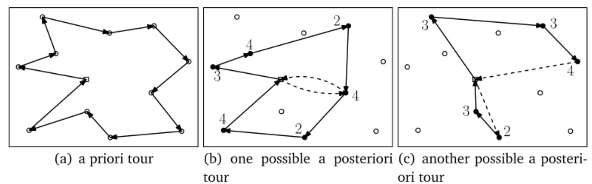
(a) a priori tour 3 2 4 4 3 2 3 3 4 2 4

(b) one possible a posteriori tour 2 3 3 ₂ 3 4 4 2 3 2 2

Figure 1.2. Example of how a posteriori tours are derived from a given a priori tour for the VRPSD. The vehicle capacity in this example is 10 and the depot is visualized by the square. Part (a) shows the given a priori tour. Parts (b) and (c) represent two particular realizations of the random events. Here the numbers denote the demands of the customers. The customers are served in the order specified by the a priori solution and the vehicle is refilled only if it gets empty. Note that if a vehicle gets empty after fully serving a customer, it is refilled at the depot and proceeds with the next customer. This happens between the last two customers in (b) and between the fourth and fifth customer in (c).

problem is a tour starting at the depot and visiting all customers exactly once. The costs for an a posteriori solution are just the total travel times. Note that here restocking actions are influencing the travel times. Figure 1.2 illustrates the relation between the a priori solution and the a posteriori solution in the context of the VRPSD.

In Bertsimas[1992] closed-form expressions and algorithms for the VRPSD objective function are given. Different interesting bounds are derived and a comparison with the corresponding reoptimization approach is performed. Ad-ditionally, the worst-case behavior of some simple heuristics is analyzed. Bas-tian and Rinnooy Kan [1992] introduces modifications of existing models and shows that under some assumptions the VRPSD exhibits the structure of the TIME-DEPENDENT TRAVELING SALESMAN PROBLEM (Lucena [1990]; Gouveia and Voß[1995]; Vander Wiel and Sahinidis [1996]). In Dror et al. [1993] a chance-constrained model and three recourse models of the VRPSD are introduced. It is shown that the chance-constrained model can be solved to optimality and that the recourse models can be solved by optimizing multiple instances of the TSP. Hjorring and Holt [1999] introduces new optimality cuts for the VRPSD. The problem is then solved using the integer L-shaped method with an

(24)

approxima-tion of the restocking costs. The integer L-shaped method is also used in Laporte et al. [2002] to solve instances of size up to 100 to optimality. In Christiansen and Lysgaard [2007] a formulation of the VRPSD as a set partitioning problem is introduced and promising results are reported. A local branching method in combination with Monte Carlo sampling is used in Rei et al. [2010]. Meta-heuristics are analyzed in Bianchi et al. [2004, 2006]; Chepuri and Homem-de Mello [2005]. While the performance of different metaheuristics are compared in Bianchi et al.[2004, 2006], Chepuri and Homem-de Mello [2005] deals with an algorithm based on the cross-entropy method. Variants with multiple goods are discussed in Mendoza et al. [2010, 2011]. A robust optimization approach is given in Sungur et al.[2008]. Finally, the problem is discussed from a reop-timization point of view in Novoa and Storer [2009]; Secomandi and Margot [2009].

We now focus on the VRPSD objective function and present the formal prob-lem definition shortly after. Let V be the set of n customers including the depot

v₁∈ V . The distances between the customers are again modeled using a function

d: V × V → R+. Let Q∈ N be the capacity of the vehicle. The demand distribu-tions can be modeled by a function g : V × 〈Q〉 → R+ withPQ_i₌₁g(v, i) = 1 for

all v ∈ V . An a prior solution can now be simply represented by a permutation

τ : 〈n〉 → V with τ1 = v1. For a given solution let Av be a random variable

describing the amount of goods in the vehicle just before customer v∈ V is pro-cessed and let Dv be a random variable describing the demand of customer v

according to the given demand distribution. With τn+1 = τ1 and Dτ1 = 0 the

expected costs ofτ can then be expressed as

fvrpsd(τ) = n X i=1 P(Aτi > Dτi) d(τi,τi+1) + n X i=1 P(Aτi = Dτi) (d(τi,τ1) + d(τ1,τi+1)) + n X i=1 P(Aτi < Dτi) (d(τi,τ1) + d(τ1,τi) + d(τi,τi+1)).

The first case corresponds to the situation in which the vehicle still contains goods after serving a customer. In that case the vehicle continues to the next customer. The second case corresponds to the situation in which the vehicle is empty after serving a customer. In this situation the vehicle returns to the depot for a restocking action and continues the tour at the next customer. The last

(25)

case corresponds to the situation in which a customer cannot be fully served. A restocking action is necessary and the vehicle travels to the depot and back to the customer. The customer is then fully served and the vehicle continues to the next customer. Note that the objective function can be computed in a runtime of O (nQ2) with a dynamic programming approach Bertsimas [1992]. That means for a fixed value of Q, which is common for this kind of problem, and even for a value of Q which is polynomially in the input size, the objective function can be computed in polynomial time. Using the mathematical expression for the objective function, we are able to state the problem as follows.

Problem 3 (VEHICLE ROUTING PROBLEM WITH STOCHASTIC DEMANDS (VRPSD)).

Given a set V of size n with a special element v₁_{∈ V , a function d : V × V → R}+, a value Q∈ N and a function g : V × 〈Q〉 → R+ withPQ_i₌₁g(v, i) = 1 for all v ∈ V , the problem is to compute a permutation τ? : 〈n〉 → V with τ?₁ = v1, such that

f_vrpsd(τ?) ≤ f_vrpsd(τ) for any permutation τ : 〈n〉 → V with τ1 = v1.

1.2.4 The Vehicle Routing Problem with Stochastic Demands

and Customers

The VEHICLE ROUTING PROBLEM WITH STOCHASTIC DEMANDS AND CUSTOMERS (VRPSDC, Gendreau et al. [1995]) is a combination of the PROBABILISTIC TRAV -ELING SALESMAN PROBLEM and the VEHICLE ROUTING PROBLEM WITH STOCHASTIC DEMANDS. In addition to the formulation of the VRPSD, the presence of the cus-tomers is modeled in a stochastic way. Depending on the context we can also see this problem as a variant of the VEHICLEROUTINGPROBLEM WITHSTOCHASTICDE -MANDSwhere we formally allow a demand of zero and customers to be skipped in this case. The relation between the a priori solution and the a posteriori so-lution for the VRPSDC is shown in figure 1.3. In the following we will omit an informal description of the problem, since the combination of the PTSP and the VRPSD is straightforward.

The literature for the VRPSDC is quite rare. A formulation of the VRPSDC as a stochastic integer program is given in Gendreau et al.[1995]. Here the integer L-shaped method is used to solve the problem to optimality. A tabu search heuristic for tackling larger instances is presented in Gendreau et al. [1996b]. Finally, a new solution approach including numerical results is given in FuCe et al.[2005]. For the formal definition of the problem we use the same notations as before. We have given a set V of n customers including the depot v1 ∈ V . A function

d : V × V → R+ is representing the distances between the customers. The capacity of the vehicle is Q ∈ N and the customers’ demands are modeled by

(26)

(a) a priori tour 4 2 4 3 2 4

(b) one possible a posteriori tour

3 3

4

2 3

Figure 1.3. Example of how a posteriori tours are derived from a given a priori tour for the VRPSDC. The vehicle capacity in this example is 10 and the depot is visualized by the square. Part (a) shows the given a priori tour. Parts (b) and (c) represent two particular realizations of the random events. Here the filled circles represent the customers that require a visit and the numbers denote the demands of these customers. The customers that require a visit are served in the order specified by the a priori solution and the vehicle is refilled only if it gets empty. Note that if a vehicle gets empty after fully serving a customer, it is refilled at the depot and proceeds with the next customer. This happens between the third and fourth customer in (c).

a function g : V × 〈Q〉 → R+ with PQ_i₌₁g(v, i) = 1 for all v ∈ V . Moreover,

a function p : V → [0, 1] represents the probabilities for the presence of the different customers. As usual, a solution is represented by a permutation τ : 〈n〉 → V with τ1= v1.

Now let τ : 〈n〉 → V be such a solution. A_v is a random variable describing the amount of goods in the vehicle just before customer v ∈ V is processed and

D_v is a random variable describing the demand of customer v according to the given demand distribution. Additionally, Nv is a random variable indicating the

next customer after v (with respect to τ) which requires to be visited. With

(27)

fvrpsdc(τ) = n X i=1 P(Aτi > Dτi) n X j=1 P(Nτi = τj) d(τi,τj) + n X i=1 P(Aτi = Dτi) d(τi,τ1) + n X j=1 P(Nτi = τj) d(τ1,τj) ! + n X i=1 P(A_τ_i < D_τ_i) d(τi,τ1) + d(τ1,τi) + n X j=1 P(N_τ_i = τj) d(τi,τj) ! .

With this expression the problem can be stated as follows.

Problem 4 (VEHICLE ROUTING PROBLEM WITH STOCHASTIC DEMANDS AND CUS

-TOMERS (VRPSDC)). Given a set V of size n with a special element v₁ ∈ V , a function d : V × V → R+, a value Q _{∈ N, a function g : V × 〈Q〉 → R}+ with

PQ

i=1g(v, i) = 1 for all v ∈ V and a function p : V → [0, 1], the problem is to

compute a permutationτ?:〈n〉 → V with τ?₁= v1, such that f_vrpsdc(τ?) ≤ f_vrpsdc(τ) for any permutationτ : 〈n〉 → V τ1= v1.

1.3 Outline

In this section we give a brief overview about the content of the subsequent chapters and the main results that are presented in this thesis.

All in all, the thesis is partitioned into a theoretical part and a practical part. The theoretical part consists of chapters 2 to 4. The results presented in these chapters are mostly about the complexity of computational tasks related to stochastic vehicle routing problems. Hardness results for the optimization problems, that are presented in this chapter, motivate the usage of heuristics for tackling these problems. Additionally, hardness results for the objective func-tions of some stochastic vehicle routing problems motivate the usage of efficient approximations for these objective functions. The practical part consists of chap-ters 5 to 8 and is motivated and partially based on the theoretical results. In chapters 5 and 6 we present heuristics for the PTSP and the PTSPD using ap-proximations of the objective functions. Comprehensive computational studies reveal the efficiency of these heuristics with respect to existing approaches. In chapter 7 we present a metaheuristic framework for solving stochastic combina-torial optimization problems using graphics processing units. A case study on the PTSPD shows that major runtime improvements can be obtained in this way.

(28)

Finally, chapter 8 deals with a real world stochastic vehicle routing problem. We introduce a model for this problem and present an efficient heuristic. This prob-lem is part of a project that has been initiated in 2010 by Caritas Suisse. The project is still in an early stage, but with our work we were able to successfully support some of the decision processes at this stage.

Note that this thesis is based on Weyland et al. [2009a,b, 2011a,b, 2012a,b,c,d, 2013a,b]. All these publications have been written by the author of this thesis under guidance and supervision of the corresponding co-authors. Weyland et al. [2012b,c, 2013b] are journal articles, Weyland et al. [2011a, 2012a] are journal articles which are currently under review and Weyland et al. [2009a,b, 2011b, 2012d, 2013a] are conference papers. At the beginning of the different sections we always refer to the corresponding publications.

(29)

Chapter 2 Convergence Results for Vehicle

Routing Problems with Stochastic

Demands

In this chapter we give convergence results for vehicle routing problems where demands are modeled in a stochastic way, like for example the VEHICLEROUTING PROBLEM WITH STOCHASTIC DEMANDS (Bertsimas[1992]) and the VEHICLEROUT -INGPROBLEM WITHSTOCHASTICDEMANDS ANDCUSTOMERS(Gendreau et al.[1995, 1996b]). The results presented here are based on the publication Weyland et al. [2013a]. These results are interesting for two reasons. On the one hand, they have an immediate impact for practical applications of vehicle routing problems with stochastic demands. We will discuss the corresponding implications at the end of this chapter. On the other hand, they are used in our analyses of the com-putational complexity of stochastic vehicle routing problems on substantially stochastic instances in chapter 3.

The remainder of this chapter is organized in the following way. We will first introduce a Markov chain model (Revuz [2005]) for vehicle routing problems with stochastic demands, which describes the amount of goods in the vehicle while the different customers are processed. Then we continue with the conver-gence results itself. Here we show that under mild conditions the distribution of the goods in the vehicle converges to the uniform distribution. This gives us a sort of asymptotic equivalence of the VEHICLE ROUTING PROBLEM WITH STOCHAS -TIC DEMANDS and the TRAVELING SALESMAN PROBLEM (Lin [1965]; Johnson and McGeoch [1997]) as well as the VEHICLE ROUTING PROBLEM WITH STOCHASTIC DEMANDS AND CUSTOMERSand the PROBABILISTIC TRAVELING SALESMAN PROBLEM (Jaillet [1985]). For practical applications it is very interesting to identify the

(30)

speed with which the distribution of goods in the vehicle converges to the uni-form distribution. We investigate this convergence speed for binomial demand distributions. After that we finish this chapter with an extensive discussion of our results.

2.1 A Markov Chain Model

In this section we introduce a Markov chain model (Revuz[2005]) that describes the amount of goods in the vehicle, which is fundamental for the remaining part of this chapter, and in particular for the proofs in the following two sections. After that we prove some properties for this model using the basic restocking strategy. For more details about Markov chains we refer to Revuz[2005].

Given the amount of goods in the vehicle before processing a certain cus-tomer, the amount of goods after the customer has been processed depends only on the demand distribution of this customer (and in the case of the VRPSDC additionally on the probability that this customer requires a visit) and is inde-pendent of the demands of the other customers. Thus it is clear that we can model the amount of goods in the vehicle for a given route with a time-discrete Markov chain, starting with a distribution representing a full vehicle, and using transition matrices that are based on the demand distributions of the customers and on the restocking strategy.

The different states represent the different amounts of goods in the vehicle. If the amount of goods is bounded from above by the vehicle capacity Q, and if we observe the amount of goods after a possible restocking action has been per-formed, it is sufficient to have different states for the amount levels 1, 2, . . . , Q, because a minimum requirement for a restocking strategy should be to perform a restocking action, if the vehicle is empty after processing a customer. For being able to use modular arithmetic in a straightforward way, we use in the following 1, 2, . . . , Q− 1 for amount levels of 1, 2, . . . , Q − 1 and 0 for an amount of Q.

That means the distribution of the amount of goods can be represented by a column vector of size Q, whose elements are all non-negative and sum up to 1. Such a vector is called stochastic (Latouche and Ramaswami [1987]). Further-more, the transition matrices are of size Q× Q and depend only on the demand distributions of the customers (and in the case of the VRPSDC additionally on the probability that the customer requires a visit), and on the restocking strategy that is used. The entry in row i and column j represents the probability that we reach state i from state j in one step. In other words, this is the probability that we have an amount of i goods after processing the customer and performing a

(31)

possible restocking action, if the amount has been j goods before processing the customer. By definition the transition matrices are stochastic in its columns, i.e. that the elements in each column sum up to 1. Note that the transition matrices for the VRPSDC are convex combinations of the corresponding transition ma-trices for the VRPSD and the identity matrix, since with a certain probability a customer is skipped and the amount of goods does not change, and otherwise the customer is served exactly as in the VRPSD.

In this chapter we focus on the basic restocking strategy which has been used in the formal definitions of the VRPSD and the VRPSDC in chapter 1. This means that we perform a restocking action if we run out of goods while processing a customer, or if the vehicle is empty after processing a customer. Therefore, the probability to reach state i from state j is the same as the probability to reach state (i + k) mod Q from state (j + k) mod Q, ∀k ∈ {1, 2, . . . ,Q − 1}. These observations lead to two additional properties for the transition matrices. Two successive rows only differ in a cyclic shift of one position, in particular for each row the following row is shifted cyclic one position to the right. The other property, which follows directly from this one for square matrices, is that the transition matrices are also stochastic in their rows, i.e. that the elements in each row sum up to 1.

Before we finish this section, we give a formal overview about the properties mentioned above, using the following definitions. For the vectors and matrices we use indices starting at 0 to allow the use of modular arithmetic in a straight-forward way.

Definition 1 (Column stochastic matrix). A m× n matrix A = (ai j) is called

stochastic in its columns, if the following two properties hold: 1. ∀i ∈ {0, 1, . . . , m − 1}, ∀ j ∈ {0, 1, . . . , n − 1} : ai j ≥ 0 2. _{∀ j ∈ {0, 1, . . . , n − 1} :} m−1 P i=0 a_{i j}= 1.

Definition 2 (Row stochastic matrix). A m×n matrix A = (ai j) is called stochastic

in its rows, if the transposed matrix AT is stochastic in its columns.

Definition 3 (Doubly stochastic matrix). A matrix A is called doubly stochastic, if

it is stochastic in its columns and stochastic in its rows.

Definition 4 (Cyclic matrix). A m× m matrix A = (ai j) is called cyclic, if the

following holds:

(32)

Now we are able to give a formal summary of the properties of the transition matrices in the following lemma.

Lemma 1. Using the Markov chain model introduced at the beginning of this

sec-tion for the VRPSD and the VRPSDC with the basic restocking strategy, the transi-tion matrices are square matrices, doubly stochastic and cyclic.

Another important fact is that column stochastic matrices, row stochastic matrices, doubly stochastic matrices and cyclic matrices are all closed under multiplication. A proof for the last statement is given in appendix A, the other statements are well known results (Latouche and Ramaswami[1987]) and easy to verify.

2.2 Convergence Results

We show in this section that there is under some mild conditions an asymptotic equivalence between the VEHICLE ROUTING PROBLEM WITH STOCHASTIC DEMANDS and the TRAVELING SALESMAN PROBLEM, as well as between the VEHICLE ROUT -INGPROBLEM WITH STOCHASTIC DEMANDS AND CUSTOMERS and the PROBABILISTIC TRAVELINGSALESMANPROBLEM.

One might think that it is important for the VRPSD and the VRPSDC to opti-mize the (expected) length of the route as well as to optiopti-mize the route in a way, such that those customers which cause a restocking action with high probability, are located close to the depot. We show that the distribution of the amount of goods in the vehicle converges to the uniform distribution under certain condi-tions. In this case the probability that restocking is required at a certain customer depends mainly on the distribution of its demand and only slightly on the par-ticular shape of the tour. In other words, if the amount of goods in the vehicle is close to the uniform distribution, it is sufficient to optimize the (expected) length of the tour.

Let us assume for the moment that the vehicle is loaded in a probabilistic way, such that the amount of goods is initially distributed according to the uniform distribution. Then the VRPSD and the TSP, and the VRPSDC and the PTSP are equivalent, if the basic restocking strategy is used. These equivalences can be verified easily using the Markov chain model introduced in the previous section. Together with the convergence of the amount of goods in the vehicle towards the uniform distribution, this observation is the basic idea behind our analyses.

(33)

We now start with a more general mathematical result. After that we show under which conditions this result can be used to derive concrete results for the VRPSD and for the VRPSDC.

Theorem 1. Let (A_n)_n_∈N be a series of doubly stochastic m× m matrices, whose

entries are all bounded from below by a constant L > 0. Then lim

n→∞ n Q i=1 A_i = 1 mJ ,

where J is a matrix of ones.

Proof. This theorem is trivially true for m = 1, so we can assume m > 1 for the following proof. Since the product of doubly stochastic matrices is a dou-bly stochastic matrix and for any doudou-bly stochastic matrix A = (ai j) we have m−1

P

j=0

a_{i j}= 1 ∀i ∈ {0, 1, . . . , m − 1} and a_{i j} ≥ 0 ∀i, j ∈ {0, 1, . . . , m − 1}, it is suffi-cient to show that the entries in each row converge to the same value. We prove this by showing that the difference between the smallest and the largest entry in each row converges to 0.

We show by induction that the difference between the smallest and the largest entry in each row of

n

Q

i=1

A_i is bounded from above by (1 − 2L)n_{. It is}

clear that this expression is always non-negative, because L is trivially bounded from above by 1/2.

For n= 1 this is clearly the case. The smallest entry is bounded from below by L and since we have doubly stochastic matrices, the largest entry is bounded from above by 1− L. The difference of the the largest entry and the smallest entry can be at most(1−L)−L = 1−2L = (1−2L)1_{. Now suppose the statement} holds for n∈ N. Here we use A(n)=

n

Q

i=1

A_i as an abbreviation for the product of the first n matrices. Let i ∈ {0, 1, . . . , m − 1} be a fixed row index and let li(n)

and ui(n) be the smallest, respectively the largest entry in the i-th row of A(n).

The entries in the i-th row of A(n+1) are convex combinations of the entries in the i-th row of A(n), where the corresponding coefficients of each of these convex combinations is a column of An+1. Since the entries of An+1 are bounded from below by L we have

u_i(n + 1) ≤ (1 − L)u_i(n) + Ll_i(n) = u_i(n) − L(u_i(n) − l_i(n)) and

l_i(n + 1) ≥ (1 − L)l_i(n) + Lu_i(n) = l_i(n) + L(u_i(n) − l_i(n)).

(34)

u_i(n + 1) − l_i(n + 1) ≤ u_i(n) − L(u_i(n) − l_i(n)) − l_i(n) − L(u_i(n) − l_i(n))

= ui(n) − li(n) − 2L(ui(n) − li(n))

= (1 − 2L)(ui(n) − li(n))

≤ (1 − 2L)n+1_.

In the last step we used the induction hypothesis and since lim

n→∞(1−2L)

n_{= 0}

we finished the proof.

In the previous section we have seen that we can model the distribution of the amount of goods in the vehicle with a Markov chain. It is possible to identify the matrices Aiof theorem 1 with transition matrices of that Markov chain. Using

the basic restocking strategy these transition matrices are doubly stochastic, but unfortunately it is a very strong assumption that their entries are all bounded from below by a constant L> 0. In this case each customer has a strictly positive probability for each possible demand and this assumption is obviously too strong for practical applications. In the remaining part of this section we show that we can use theorem 1 also under more moderate conditions.

The main idea here is to partition the matrices into blocks of consecutive matrices, such that the product of all the matrices within a block fulfills the con-ditions of theorem 1. Due to the associative law the product of all the matrices can be obtained by first calculating the products of the matrices within each block and then multiplying the resulting products. In this way we are able to state theorem 1 using much weaker assumptions on the matrices used. These weaker assumptions are comprised in the following definition and as we will see later, it is not even required that these assumptions hold for all of the matrices.

Definition 5 (greatest common divisor property, gcd property). A cyclic m× m

matrix A= (a_{i j}) with only non-negative entries and with strictly positive entries a_i

10, ai20, . . . , ail0, i1< i2< . . . < il in the first column fulfills the greatest common divisor property (short: gcd property), ifgcd(i_l− i1, i_l− i2, . . . , i_l− il−1, m) = 1.

Instead of using the differences relative to i_l we could have also used differ-ences relative to any other of the elements i_k, k ∈ {1, 2, . . . , l}. The definition is also invariant with respect to the chosen column. We prove both invariances in appendix A.

At first glance this definition looks quite technical, but it is usually fulfilled by a lot of the transition matrices for practical instances of the VRPSD and the

(35)

VRPSDC. In particular, the greatest common divisor property is fulfilled for a transition matrix, if the corresponding customer has two different demands of amount k and k+ 1 with strictly positive probabilities. For the VRPSDC we have always a strictly positive entry at the first position in the first column (unless the probability for visiting this customer is exactly 1) and therefore the condition is even slightly weaker in this case. We discuss this issue more in detail in section 2.4. Here we continue with deriving a convergence result as in theorem 1 under more mild assumptions comprised by the gcd property.

We start with proving the following important lemma using the definition of the gcd property and some modular arithmetic.

Lemma 2. Let A be a m× m matrix with only non-negative entries and with ki

strictly positive entries in row i, i ∈ {0, 1, . . . , m − 1}, and let B be a cyclic m × m

matrix with only non-negative entries fulfilling the greatest common divisor prop-erty. Then the product C = AB contains only non-negative entries and has at least

min{ki+ 1, m} strictly positive entries in row i, for each i ∈ {0, 1, . . . , m − 1}.

Proof. The elements of the set I = {i1, i2, . . . , in} ⊂ Z/mZ, n ∈ N, with

gcd(i1, i₂, . . . , i_n, m) = 1 can be used to generate any element of Z/mZ by a linear combination of i1, i2, . . . , in. This is a well known algebraic result, see e.g.

Baldoni et al.[2008].

For our proof we need the following useful property. Given a set S⊂ Z/mZ with|S| < |Z/mZ|, and I as above, then for the set S0_{= {s+i | s ∈ S, i ∈ I ∪{0}}} the inequality |S| < |S0| holds. Otherwise we cannot generate all elements of Z/mZ by linear combinations of i1, i2, . . . , in.

Let i∈ {0, 1, . . . , m − 1} be a fixed row index with ki < m, let S = {j | ai j >

0} ⊂ Z/mZ and let S0_{= {j | c}

i j > 0} ⊂ Z/mZ. Furthermore let bj10, bj20, . . . , bjl0, j1 < j2 < . . . < jl be the strictly positive entries in the first column of B. Due to

the properties of our matrices, we have S0 = {(s + b) mod m | s ∈ S, b = − j_i, i∈ {1, 2, . . . , l}} = {(s − j_l+ b) mod m | s ∈ S, b = j_l− j_i, i∈ {1, 2, . . . , l}} = {(s − j_l+ b) mod m | s ∈ S, b ∈ {j_l− j1, j_l− j2, . . . , j_l− j_l₋₁} ∪ {0}} = {(s + b) mod m | s ∈ S, b ∈ { j_l− j1, j_l− j2, . . . , j_l− j_l₋₁} ∪ {0}} > |S| ,

which concludes the proof for all rows with less than m strictly positive entries. Now let i ∈ {0, 1, . . . , m − 1} be a fixed row index with ki = m. Since each

(36)

entries in the i-th row of C = AB is m which concludes the proof for rows with exactly m strictly positive entries.

Using this lemma we can obtain a sufficient condition for the case that the product of a number of transition matrices contains only strictly positive entries.

Corollary 1. Let A1, A2, . . . , Ak be cyclic m× m matrices with only non-negative

entries and with at least 1 strictly positive entry in each row, and let m− 1 of these

matrices fulfill the greatest common divisor property. Then B=

k

Q

i=1

A_i contains only strictly positive entries.

Proof. Since the matrices are cyclic and have at least 1 strictly positive entry in each column the number of strictly positive entries in the series of products is never decreasing in any of the rows. Due to lemma 2 a multiplication with one of the matrices, which fulfills the gcd property, increases the number of strictly positive entries in each row by at least 1 (if it has not been maximum already). Putting these observations together the corollary follows easily.

To generalize the convergence result of theorem 1 we need the following lemma.

Lemma 3. Let A= (a_{i j}) be a m×m matrix containing only strictly positive entries,

with a smallest entry l and a largest entry u and let B be a m× m column stochastic

matrix. Then u0_−l0_{≤ u−l, where u}0and l0are the largest, respectively the smallest, strictly positive entries in AB.

Proof. The elements of AB are convex combinations of elements of A and there-fore the elements of AB are bounded from below by l and from above by u.

Now we are able to generalize the convergence result of theorem 1.

Theorem 2. Let (A_n)_n_∈N be a series of doubly stochastic, cyclic m× m matrices,

whose entries are all bounded from below by a constant L > 0. Let the great-est common divisor property be fulfilled by infinitely many of these matrices and let k₁ < k₂ < . . . be the indices of the matrices that fulfill the gcd property. If

max{ki+1− ki | i ∈ N} ≤ k for a constant k ≥ k1 then lim n→∞ n Q i=1 A_i = 1 mJ , where J is a matrix of ones.

Proof. To proof this theorem we have to combine the previous results. Here we show like in theorem 1 that the differences between the largest and the

(37)

smallest element in each row of the successive products

n

Q

i=1

A_i are monotonically decreasing and converge to 0.

It is possible to partition the matrices into blocks of at most k(m − 1) con-secutive matrices, such that the matrices in each block fulfill the conditions of corollary 1. Let 1 = j1 < j2 < . . . be the indices at which the first, second, . . . block begins. Then we can bound the smallest entry of the products

jl+1−1

Q

i=jl A_i by

L0= Lk(m−1).

We can now create a new series(B_n)_n_∈N, with

B_n:=

jn+1−1

Y

i=jn A_i.

Due to corollary 1 these matrices fulfill the conditions of theorem 1 and thus we have lim n→∞ n Q i=1 B_i = 1

mJ. Analogue to the proof of theorem 1 we can now bound

the difference between the largest and the smallest element in each row of the product n Q i=1 B_i = jn+1−1 Q i=1

A_i from above by(1 − 2L0)n. With lemma 3 we can show that the difference between the largest and the smallest element of

j

Q

i=1

A_i can also be bounded from above by(1 − 2L0)n, if jn+1 ≤ j < jn+2− 1. This concludes

the proof.

Let us quickly connect these results with the original stochastic vehicle rout-ing problems. What we have seen on a more abstract level is the followrout-ing. If we impose some mild conditions on the transition matrices of our Markov chain model, the amount of goods in the vehicle after a customer has been processed is approaching the uniform distribution as we continue on the tour and more and more customers are visited. For the basic restocking strategy which we are using here, the transition matrices are characterized only by the customers’ de-mands (and in the case of the VRPSDC additionally by the probability that the customers require to be visited). Therefore, the mild conditions on the transition matrices are transferred to mild conditions on the customers’ demands. At the very beginning of this chapter we have already observed that it is sufficient to optimize the (expected) length of the route if the amount of goods in the vehicle is distributed according to the uniform distribution. Together with our conver-gence result, this shows that it is sufficient to focus on optimizing the (expected) length of the route in many situations. In the next section we will examine the