1
Abstract— In this paper the Model Predictive control (MPC) for
the improvement of the power system stability is presented. Particularly, the paper focus on the application of the MPC technique to regulate the power output of the generators when the system is subject to fault and disturbances.
The application on the Single machine infinite bus equipped with Thyristor Controlled Series Capacitor device is carried out to show the advantage of the proposed technique.
Index Terms—MPC, TCSC, SMIB and Transient Stability.
I. INTRODUCTION
EVERAL control problems can be formalized under the form of optimal control problems having discrete-time dynamics and costs that are additive over time. Model Predictive control (MPC) is an approach to solve such problems. MPC was originally designed to exploit an explicitly formulated model of the process and solve in a receding horizon manner a series of open-loop deterministic optimal control problems [1], [2]. The main motivation behind the research in MPC was initially to find ways to stabilize large-scale systems with constraints around some equilibrium points (or trajectories) [3][4].
MPC is an advanced method of process control that has been in use in the process industries such as chemical plants and oil refineries since the 1980s. Model predictive controllers rely on dynamic models of the process, most often linear empirical models obtained by system identification.
The models used in MPC are generally intended to represent the behavior of complex dynamical systems. The additional complexity of the MPC control algorithm is not generally needed to provide adequate control of simple systems, which are often controlled well by generic PID controllers. Common dynamic characteristics that are difficult for PID controllers include large time delays and high-order dynamics.
MPC models predict the change in the dependent variables of the modeled system that will be caused by changes in the independent variables. In a chemical process, independent variables that can be adjusted by the controller are often either
Dr Karim Sebaa, Samir Moulahoum and Hamza Houassin are with Electrical Engineering Department, University of Médéa, Cité Ain d’hab, 26000 Médéa, Algeria. (Phone: +213-553-54-5033 e-mail: [email protected]).
the setpoints of regulatory PID controllers (pressure, flow, temperature, etc.) or the final control element (valves, dampers, etc.). Independent variables that cannot be adjusted by the controller are used as disturbances. Dependent variables in these processes are other measurements that represent either control objectives or process constraints.
MPC uses the current plant measurements, the current dynamic state of the process, the MPC models, and the process variable targets and limits to calculate future changes in the independent variables. These changes are calculated to hold the dependent variables close to target while honoring constraints on both independent and dependent variables. The MPC typically sends out only the first change in each independent variable to be implemented, and repeats the calculation when the next change is required.
While many real processes are not linear, they can often be considered to be approximately linear over a small operating range. Linear MPC approaches are used in the majority of applications with the feedback mechanism of the MPC compensating for prediction errors due to structural mismatch between the model and the process. In model predictive controllers that consist only of linear models, the superposition principle of linear algebra enables the effect of changes in multiple independent variables to be added together to predict the response of the dependent variables. This simplifies the control problem to a series of direct matrix algebra calculations that are fast and robust.
When linear models are not sufficiently accurate to represent the real process nonlinearities, several approaches can be used. In some cases, the process variables can be transformed before and/or after the linear MPC model to reduce the nonlinearity. The process can be controlled with nonlinear MPC that uses a nonlinear model directly in the control application. The nonlinear model may be in the form of an empirical data fit (e.g. artificial neural networks) or a high-fidelity dynamic model based on fundamental mass and energy balances. The nonlinear model may be linearized to derive a Kalman filter or specify a model for linear MPC.
In this paper; the theoretical description of MPC is provided and an application to SMIB equipped with TCSC is illustrated with various projection length where it is demonstrated that the prediction horizon choice is difficult. Prediction too far into the future is computationally expensive and sometimes not useful due to plant uncertainty.
Model Predictive Control to improve the power
system stability
K. Sebaa, S. Moulahoum and H. Houassin
2
II. MODEL PREDICTIVE CONTROL
1) Theory behind MPC
MPC is based on iterative, finite horizon optimization of a plant model. At time t the current plant state is sampled and a cost minimizing control strategy is computed (via a numerical minimization algorithm) for a relatively short time horizon in the future: [t, t + T]. Specifically, an online or on-the-fly calculation is used to explore state trajectories that emanate from the current state and find (via the solution of Euler-Lagrange equations) a cost-minimizing control strategy until time t + T. Only the first step of the control strategy is implemented, then the plant state is sampled again and the calculations are repeated starting from the now current state, yielding a new control and new predicted state path. The prediction horizon keeps being shifted forward and for this reason MPC is also called receding horizon control. Although this approach is not optimal, in practice it has given very good results. Much academic research has been done to find fast methods of solution of Euler-Lagrange type equations, to understand the global stability properties of MPC's local optimization, and in general to improve the MPC method. To some extent the theoreticians have been trying to catch up with the control engineers when it comes to MPC[1].
Fig. 1. A discrete MPC scheme.
1) Principles of MPC
Model Predictive Control (MPC) is a multivariable control algorithm that uses:
an internal dynamic model of the process a history of past control moves and
an optimization cost function J over the receding prediction horizon,
to calculate the optimum control moves. The optimization cost function is given by:
min u[1:::k]2UJ = Np X k=1 wx(r[k] ¡ x[k])2+ Np X k=1 wu¢u[k]2] min u[1:::k]2UJ = Np X k=1 wx(r[k] ¡ x[k])2+ Np X k=1 wu¢u[k]2] (1) without violating constraints (low/high limits)
With: x[k]
x[k] controlled variable (e.g. measured temperature) r[k]
r[k] reference variable (e.g. required temperature) u[k]
u[k] manipulated variable (e.g. control valve) wx
wx weighting coefficient reflecting the relative of xx
wu
wu weighting coefficient reflecting the relative of uu
U
U is the set of control values Np
Np is the projection length
III. APPLICATION
A) Test system (SMIB)
The MPC control is applied on the SMIB power system with TCSC as shown in Fig. 2 The input control of this system study is the TCSC’s reactance. The synchronous generator is delivering power to the infinite-bus through a double circuit transmission line and a TCSC. In Fig. 2, VVtt and EEbbare the generator terminal and infinite bus voltage respectively; XXTT, XXLL and XXT HT H represent the reactance of the transformer, transmission line per circuit and the Thevenin’s impedance of the receiving end system respectively.
Fig. 2 Single-machine infinite-bus power system with TCSC
The synchronous generator is represented by model 1.1, i.e. with field circuit and one equivalent damper winding on q-axis.
The machine equations with AVR are [5]:
8 > > > > > > < > > > > > > : d± dt = !B£ (Sm¡ Smo) dxm dt = 1 2£H[¡D £ (Sm¡ Smo) + Tm¡ Te dE0q dt = 1 T0 do [¡E0 q+ (xd¡ x0d) £ id+ Ef d] dE0d dt = 1 T0 qo[¡E 0 d+ (xq¡ x0q) £ iq] Ef d dt = 1 TA[¡Efd+ KA£ (Vref¡ Vt)] 8 > > > > > > < > > > > > > : d± dt = !B£ (Sm¡ Smo) dxm dt = 1 2£H[¡D £ (Sm¡ Smo) + Tm¡ Te dE0q dt = 1 T0 do [¡E0 q+ (xd¡ x0d) £ id+ Ef d] dE0d dt = 1 T0 qo[¡E 0 d+ (xq¡ x0q) £ iq] Ef d dt = 1 TA[¡Efd+ KA£ (Vref¡ Vt)]
For more details, the readers are suggested to refer [5,6].
Fig. 3. SMIB without control
(A three phase fault is applied at the generator terminal busbar at t = 1 sec and cleared after 5 cycles. The original system is restored upon the fault clearance and an increment of Power demande from 0.6 pu to 1 pu at 5 sec)
0 1 2 3 4 5 6 7 8 9 10 -4 -2 0 2 4 0 1 2 3 4 5 6 7 8 9 -0.1 -0.05 0 0.05
3
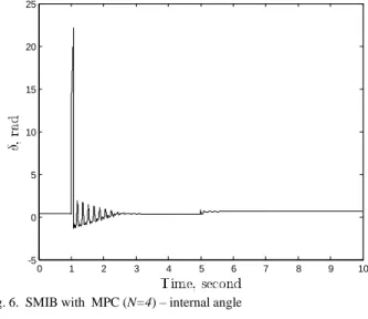
It is clear from Fig. 3 that without TCSC modulation the system is very stressed and oscillatory.
The MPC strategy will be used in next, where the controlled variable is the electrical power (x[k] = Px[k] = Pee[k][k]) and the manipuled variable is the TCSC’s reactance (u[k] = xu[k] = xT CSCT CSC[k][k] ). kk is the sample time. The weighting coefficient are
wx= 0:1 wx= 0:1andwwuu= 0:1= 0:1. u[k] = 8 > < > : +0:8 £ xline if xT CSC¸ +0:8 £ xline ¡0:2 £ xline if xT CSC· ¡0:2 £ xline xT CSC[k] otherwise u[k] = 8 > < > : +0:8 £ xline if xT CSC¸ +0:8 £ xline ¡0:2 £ xline if xT CSC· ¡0:2 £ xline xT CSC[k] otherwise
We use the cost function (1) with N = 4 (for 0.004 seconds projection into the future), wwxx= 1= 1 and wwuu= 1= 1. Also, we assume at each time instant that the reference input remains constant while we project into the future; this is equivalent to assuming that our evaluation of which controller is best is based on the reference input being constant.
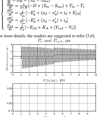
Fig. 4. SMIB with MPC (N=4) – Electrical power and TCSC reactance
Fig. 5. SMIB with MPC (N=4) – Voltage profile
Fig. 6. SMIB with MPC (N=4) – internal angle
Fig. 7. SMIB with MPC (N=4) – machine speed
To see how the MPC strategy operates, see Figure 4. Here, we see that we get a slower rise-time. It was possible to tune the MPC performance by adjusting wwxx and wwuu.
B) Effects of Planning Horizon Length
Next, we return to using the parameters for the nominal plant and study the effect of changing the projection length N with all the same choices. In particular, we plot the tracking energy. 1 2 X k (Pe[k] ¡ Peref)2 1 2 X k (Pe[k] ¡ Peref)2
And control energy 1 2 X k xT CSC[k]2 1 2 X k xT CSC[k]2 vs. N 2 f1; 2; 3; 4; 5; 6; 8; 10; 1215; 20; 22; 25; 30; 40; 45g N 2 f1; 2; 3; 4; 5; 6; 8; 10; 1215; 20; 22; 25; 30; 40; 45g 0 1 2 3 4 5 6 7 8 9 10 -4 -2 0 2 4 6 0 1 2 3 4 5 6 7 8 9 -0.1 -0.05 0 0.05 0 1 2 3 4 5 6 7 8 9 10 0 0.2 0.4 0.6 0.8 1 1.2 1.4 0 1 2 3 4 5 6 7 8 9 10 -5 0 5 10 15 20 25 0 1 2 3 4 5 6 7 8 9 10 -0.2 -0.1 0 0.1 0.2 0.3 0.4 0.5
4
Fig. 8. Tracking energy vs. projection length NN .
as shown in Fig. 8 and 9. This range of N was chosen by adding more points where the values of the tracking and control energy changed fast.
These plots show some justification for the choice of N = 2 in our simulations. This choice did not cost too much computational complexity in projecting into the future, and yet gave a low tracking error (our main objective), with a reasonable amount of control energy. If you are not concerned about computational complexity, you may want to further increase the planning horizon, to get a similar value for the tracking energy, but with even lower control energy.
Fig. 9. Control energy vs. projection length NN
Why did the values of the control energy change so quickly around the value of N = 4? Why does the tracking energy increase in the region from N = 10 to N = 16? Why is it the case that the control energy increases from N = 5 to N = 25? In general, how do you change the shape of the plots? Clearly,
changing the w1 and w2 weights will change the shape, and hence, what choices you might make for what you call a ―best‖ value of N. The model used for prediction, and the types of controllers that are simulated into the future will also change the shape. Moreover, the reference input can change it. Even though the generation of such plots can help you choose the planning horizon, it does not completely solve the problem. It simply provides insights.
Finally, in some cases it is possible that longer planning horizons can actually degrade performance since the longer you simulate into the future with an inaccurate model, the less reliable the predictions tend to be. Hence, the optimization for plan choice can become inappropriate for selecting a good plan.
IV. CONCLUSION
In this paper, the application of MPC strategy to improve the stability of the SMIB plant via the TCSC modulation is performed and discussed , also the impact of projection length on the Control energy and tracking error is presented.
V. APPENDIX
System data: All data are in pu unless specified otherwise. Generator:H = 3:542H = 3:542, D = 0; XD = 0; Xdd= 1:7572; X= 1:7572; Xqq= 1:5845= 1:5845, X0 d= 0:4245; Xq0 = 1:04; Tdo0 = 6:66; Tqo0 = 0:44; Ra= 0; Pe= 0:6; Qe= 0:02224; ±0= 44:370: X0 d= 0:4245; Xq0 = 1:04; Tdo0 = 6:66; Tqo0 = 0:44; Ra= 0; Pe= 0:6; Qe= 0:02224; ±0= 44:370: Exciter: KKAA= 400; T= 400; TAA= 0:025s= 0:025s Transmission line: R = 0; XL= 0:8125; XT = 0:1364; XT H= 0:13636; G = 0; B = 0; R = 0; XL= 0:8125; XT = 0:1364; XT H= 0:13636; G = 0; B = 0; REFERENCES
[1] M. Morari and J. H. Lee, ―Model predictive control: Past, present and future,‖ Comput. Chem. Eng., vol. 23, no. 4, pp. 667–682, May 1999. [2] J. Maciejowski, Predictive Control With Constraints. Englewood Cliffs, NJ: Prentice-Hall, 2001.
[3] D.Mayne and J. Rawlings, ―Constrained model predictive control: Stability and optimality,‖ Automatica, vol. 36, no. 6, pp. 789–814, Jun. 2000.
[4] D. Ernst, M. Glavic, F. Capitanescu and L. Wehenkel " Reinforcement learning versus model predictive control: a comparison on a power system problem ".. IEEE Transactions on Systems, Man, and Cybernetics - Part B: Cybernetics, Volume 39, Issue 2, April 2009, Page(s):517 - 529. [5] K. R. Padiyar, Power System Dynamics Stability and Control,
BS Publications, 2nd Edition, Hyderabad, India, 2002.
[6] P. Kundur, Power System Stability and Control. New York: McGraw- Hill, 1994. 0 5 10 15 20 25 30 35 40 45 1000 1500 2000 2500 3000 3500 4000 4500 5000 5500 0 5 10 15 20 25 30 35 40 45 5 10 15 20