Advanced mixed-integer programming formulations : methodology, computation, and application

Advanced mixed-integer programming formulations:

Methodology, computation, and application

by

Joseph Andrew Huchette

B.A., Rice University (2013)

Submitted to the Sloan School of Management

in partial fulfillment of the requirements for the degree of

Doctor of Philosophy

at the

MASSACHUSETTS INSTITUTE OF TECHNOLOGY

June 2018

© Massachusetts Institute of Technology 2018. All rights reserved.

Author . . . .

Sloan School of Management

May 15, 2018

Certified by. . . .

Juan Pablo Vielma

Richard S. Leghorn (1939) Career Development Associate Professor of

Operations Research

Thesis Supervisor

Accepted by . . . .

Dimitris Bertsimas

Boeing Professor of Operations Research

Codirector, Operations Research Center

Advanced mixed-integer programming formulations:

Methodology, computation, and application

by

Joseph Andrew Huchette

Submitted to the Sloan School of Management on May 15, 2018, in partial fulfillment of the

requirements for the degree of Doctor of Philosophy

Abstract

This thesis introduces systematic ways to use mixed-integer programming (MIP) to solve difficult nonconvex optimization problems arising in application areas as varied as operations, robotics, power systems, and machine learning. Our goal is to produce MIP formulations that perform extremely well in practice, requiring us to balance qualities often in opposition: formulation size, strength, and branching behavior.

We start by studying a combinatorial framework for building MIP formulations, and present a complete graphical characterization of its expressive power. Our ap-proach allows us to produce strong and small formulations for a variety of structures, including piecewise linear functions, relaxations for multilinear functions, and obstacle avoidance constraints.

Second, we present a geometric way to construct MIP formulations, and use it to investigate the potential advantages of general integer (as opposed to binary) MIP formulations. We are able to apply our geometric construction method to piecewise linear functions and annulus constraints, producing small, strong general integer MIP formulations that induce favorable behavior in a branch-and-bound algorithm.

Third, we perform an in-depth computational study of MIP formulations for non-convex piecewise linear functions, showing that the new formulations devised in this thesis outperform existing approaches, often substantially (e.g. solving to optimality in orders of magnitude less time). We also highlight how high-level, easy-to-use com-putational tools, built on top of the JuMP modeling language, can help make these advanced formulations accessible to practitioners and researchers. Furthermore, we study high-dimensional piecewise linear functions arising in the context of deep learn-ing, and develop a new strong formulation and valid inequalities for this structure.

We close the thesis by answering a speculative question: Given a disjunctive constraint, what can we reasonably sacrifice in order to construct MIP formulations with very few integer variables? We show that, if we allow our formulations to introduce spurious “integer holes” in their interior, we can produce strong formulations for any disjunctive constraint with only two integer variables and a linear number of inequalities (and reduce this further to a constant number for specific structures).

We provide a framework to encompass these MIP-with-holes formulations, and show how to modify standard MIP algorithmic tools such as branch-and-bound and cutting planes to handle the holes.

Thesis Supervisor: Juan Pablo Vielma

Title: Richard S. Leghorn (1939) Career Development Associate Professor of Opera-tions Research

Acknowledgments

This thesis would certainly not exist without the guidance of my advisor, Juan Pablo Vielma. His energy and excitement are an inspiration, and he has always guided me towards interesting problems, while allowing me the freedom to explore them once I get there. He has been incredibly generous with his time and financial support, and the extent to which I have been able to travel, meet interesting people, and present my work to others has undoubtedly made me a much better researcher and academic. I thank him for serving as an exemplar of the advisor I hope to be in the coming years.

I would also like to thank Jim Orlin and Michel Goemans for serving on my thesis committee. In particular, their insightful comments and suggestions on early presentations of this work helped me immeasurably in communicating its main ideas as effectively as possible.

The Operations Research Center is a special place, entirely because of the peo-ple found behind its doors. Dimitris and Patrick deserve commendation for their leadership and vision, as do Laura and Andrew for ensuring that everything runs as smoothly as it does. My fellow students are brilliant, but also fun, interesting, and grounded, and I am grateful to have made so many great friends during my time here. I would like to thank my coauthors during my time at MIT–especially Santanu Dey and Cosmin Petra–for their guidance and mentorship early during my PhD. I am also indebted to my undergraduate professors at Rice for seeding my interest in mathematics and operations research, and especially Beatrice Riviere and Hadley Wickham for their mentorship as I took my first steps as a researcher. I owe a special thanks to Miles and Iain for starting JuMP and recruiting me to join before any of us really knew where it was headed. It’s been fantastic to have something “fun” to work on besides my research, and that it has blossomed into something others find useful makes it all the more rewarding.

I would like to thank all my friends–from all stages of life, in Cambridge and elsewhere–for making life interesting. You all have make the past five years as

enjoy-able as they have been.

I am especially grateful to have had Elisabeth in my life these past two years: as my travel companion, research commiserator, and partner.

Finally, without the support of my parents and family–for as long as I can remem-ber, and before that too, I’m sure–I certainly wouldn’t be the person I am today.

Contents

1 Preliminaries. 21

1.1 Mixed-integer programming and formulations . . . 21

1.2 Disjunctive constraints . . . 23

1.2.1 Combinatorial disjunctive constraints . . . 24

1.2.2 Combinatorial disjunctive constraints and data independence . 26 1.3 Motivating problems . . . 27

1.3.1 Modeling discrete alternatives . . . 27

1.3.2 Piecewise linear functions . . . 28

1.3.3 The SOS𝑘 constraint . . . 34

1.3.4 Cardinality constraints . . . 34

1.3.5 Discretizations of multilinear functions . . . 34

1.3.6 Obstacle avoidance constraints. . . 36

1.3.7 Annulus constraints. . . 37

1.3.8 Optimizing over trained neural networks . . . 38

1.4 Assessing the quality of MIP formulations . . . 39

1.4.1 Strength . . . 39

1.4.2 Size . . . 41

1.4.3 Branching behavior . . . 41

1.5 Existing approaches . . . 44

1.6 Contributions of this thesis . . . 46

2 A combinatorial way to construct formulations. 51

2.1 Independent branching schemes . . . 52

2.2 What does independent branching mean? . . . 53

2.2.1 Constraint branching via independent branching schemes . . . 53

2.2.2 Independence in formulation-induced branching schemes . . . 55

2.3 Independent branching scheme representability . . . 58

2.3.1 A graphical characterization . . . 58

2.3.2 Cardinality constraints . . . 60

2.3.3 Polygonal partitions of the plane . . . 60

2.3.4 Pairwise IB-representable constraints . . . 63

2.4 Pairwise independent branching schemes . . . 66

2.4.1 Graphical representations of pairwise IB-representable CDCs . 66 2.4.2 Representation at a given depth . . . 67

2.5 A simple IB scheme and its limitations . . . 71

2.6 Systematic construction of biclique covers . . . 74

2.7 Biclique covers for graph products and discretizations of multilinear functions . . . 77

2.8 Completing biclique covers via graph unions . . . 79

2.8.1 Grid triangulations of the plane . . . 81

2.8.2 Higher-dimensional grid triangulations . . . 84

2.8.3 An even smaller formulation for bivariate grid triangulations . 85 2.8.4 The SOS𝑘 constraint . . . 88

3 Building formulations geometrically: Embeddings. 95 3.1 The embedding approach . . . 95

3.2 How many integer variables do we need? . . . 97

3.2.1 A geometric characterization of when embeddings yield valid formulations . . . 104

3.3 A geometric construction for ideal formulations of any combinatorial

disjunctive constraint . . . 107

3.4 Novel MIP formulations for univariate piecewise linear functions . . . 113

3.5 Small MIP formulations for the annulus. . . 117

4 MIP formulations for nonconvex piecewise linear functions. 123 4.1 Univariate piecewise linear functions . . . 123

4.1.1 Univariate computational experiments . . . 124

4.1.2 Branching behavior of MIP formulations . . . 128

4.2 New hybrid formulations for bivariate piecewise linear functions . . . 135

4.2.1 The combination of ideal formulations . . . 135

4.2.2 Bivariate computational experiments . . . 138

4.2.3 Optimal independent branching schemes . . . 140

4.3 Computational tools for piecewise linear modeling: PiecewiseLinearOpt142 4.4 Preliminary extensions: MIP formulations for neural networks . . . . 146

4.4.1 Existing formulations . . . 146

4.4.2 An ideal formulation for a single ReLu . . . 147

4.4.3 A separation procedure . . . 152

4.4.4 Valid inequalities for multiple layers . . . 154

5 Very small formulations and the MIP-with-holes approach. 157 5.1 Branching schemes and MIP-with-holes formulations . . . 160

5.2 Choices of encodings . . . 163

5.2.1 The reflected binary Gray and zig-zag encodings . . . 163

5.2.2 The moment curve encoding . . . 163

5.2.3 A more exotic encoding . . . 164

5.3 Very small MIP-with-holes formulations . . . 167

5.3.1 A big-𝑀 MIP-with-holes formulation for any disjunctive set . 169 5.3.2 A very small formulation for the SOS1 constraint . . . 170

5.3.3 Very small formulations for general combinatorial disjunctive constraints. . . 171

5.3.4 A very small formulation for the SOS2 constraint . . . 174

5.3.5 A very small formulation for the annulus . . . 179

A The logarithmic formulation of Misener et al. [106] is not ideal 181

B Constructing a pairwise IB-representable partition of the plane 183

C 8-segment piecewise linear function formulation branching 187

List of Figures

1-1 (Left) A univariate piecewise linear function, and (Right) a bivariate piecewise linear function with a grid triangulated domain.. . . 28

1-2 Three grid triangulations of Ω “ r1, 3s ˆ r1, 3s: (Left) the Union Jack (J1) [127], (Center) the K1 [84], and (Right) a more idiosyncratic triangulation. . . 32

1-3 Two bivariate functions over 𝐷 “ r0, 1s2 _{that match on the gridpoints,}

but differ on the interior of 𝐷. . . 33

1-4 A trajectory for a UAV which avoids an obstacle in the center of the domain. . . 36

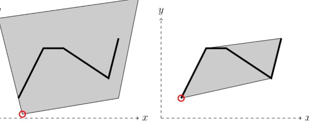
1-5 (Left) The annulus 𝒜 and (Right) its corresponding quadrilateral relaxation ˆ𝒜 given by (1.14) with 𝑑 “ 8. . . 37 1-6 The relaxations (gray region) for two different formulations of a

non-convex set (solid lines), corresponding a univariate piecewise linear function. (Left) One is not sharp, while (Right) the second is sharp. If we solve the relaxted optimization problem minp𝑥,𝑦qP𝑅𝑦 for each

re-laxation 𝑅, we get different optimal solution values (optimal solutions circled), and therefore different dual bounds for the MIP problem. . . 40

1-7 (Top) Good branching for one formulation of a univariate piecewise linear function, and (Bottom) bad, unbalanced branching from an-other formulation. . . 42

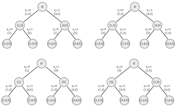
2-1 The branch-and-bound trees for (Left) (2.4) and (Right) (2.5), when (Top row) 𝑧1 is first to branch on, and then 𝑧2, and when (Bottom

row) 𝑧2 is first to branch on, and then 𝑧1. Inside each node is the set

𝐼 Ă_{J5K of all components 𝑣 for which the algorithm has been able prove} that 𝜆𝑣 “ 0 at this point in the algorithm via branching decisions. The

text on the lines show the current branching decision (e.g. 𝑧2 ě 1),

and the set of components 𝑣 PJ5K for which the (a) subproblem is able to prove that 𝜆𝑣 “ 0 independently of any other branching decisions

(e.g. 𝑧2 ě 1 is the only additional branching constraint added to the

original relaxation). This figure is adapted from [135, Figure 2]. . . . 57

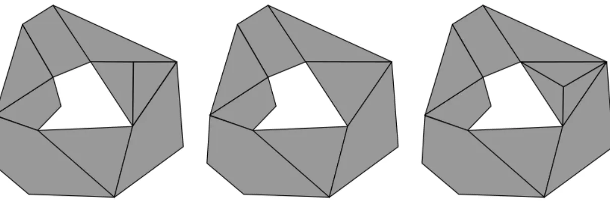
2-2 Partitions of a nonconvex region in the plane obtained by removing a central non-convex portion from a convex polyhedron. (Left) The first partition does not satisfy the internal vertices condition (2.7), (Cen-ter) the second partition admits a pairwise IB scheme, and (Right) the third partition admits a 3-way IB scheme but not a pairwise one. 63

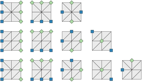
2-3 Visualizations of the biclique covers presented in the text for (Left) SOS3p6q and (Right) SOS3p10q. Each row corresponds to some level 𝑗, and the elements of 𝐴𝑗 and 𝐵𝑗 are the blue squares and green diamonds,

respectively. . . 73

2-4 The recursive construction for biclique covers for SOS2. The first row is a single biclique that covers the conflict graph for SOS2(3) (𝐴1,1in blue,

𝐵1,1in green). The second row shows the construction which duplicates the ground set t1, 2, 3u and inverts the ordering on the second copy. The third row shows the identification of the nodes that yields a valid biclique for SOS2(5). This biclique is then combined with a second that covers all edges between nodes identified with the first copy and those identified with the second, giving a biclique cover for SOS2(5) with two levels. . . 75

2-5 Independent branching schemes for the three triangulations presented in Figure 1-2, each given its own row.The sets 𝐴𝑗 and 𝐵𝑗 are given by

the blue squares and green diamonds, respectively, in the 𝑖-th subfigure of the corresponding row.. . . 80

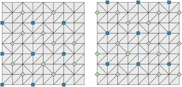
2-6 Two bicliques constructed via Corollary 5 for a grid triangulation with 𝑑1 “ 𝑑2 “ 8. On the left the construction follows by taking 𝑢 “ p1, 1q;

on the right, with 𝑢 “ p2, 3q. For each level, the sets 𝐴p𝑢q and 𝐵p𝑢q are given by the blue squares and green diamonds, respectively. . . . 83

2-7 The aggregated SOS2 independent branching formulation for subrect-angle selection. The sets 𝐴1,𝑘 _{(resp. 𝐵}1,𝑘_{) are the squares (resp.}

di-amonds) in the first row; similarly for the sets 𝐴2,𝑘 _{and 𝐵}2,𝑘 _{in the}

second row. . . 89

2-8 The 6-stencil triangle selection independent branching formulation. The sets 𝐴𝐷𝐿,𝛼 (resp. 𝐵𝐷𝐿,𝛼) are the squares (resp. diamonds) in

the first row; similarly for the sets 𝐴𝐴𝐷𝐿,𝛼 _{and 𝐵}𝐴𝐷𝐿,𝛼 _{in the second}

row. The diagonal/antidiagonal lines considered in each level are circled. 89

2-9 Visualizations of the biclique cover from the proof of Theorem 7 for SOS3p26q. Each row corresponds to some level 𝑗, and the sets 𝐴𝑗

and 𝐵𝑗 _{are the blue squares and green diamonds, respectively. The}

first three rows correspond the the “first stage” of the biclique cover tp𝐴1,𝑗, 𝐵1,𝑗qu3𝑗“1, and the second nine correspond to the “second stage”

tp𝐴2,𝑗, 𝐵2,𝑗qu9𝑗“1. . . 92

3-1 Two embeddings with the encoding 𝐻 “ p1, 2, 3q and different or-ders of the sets as (Left) 𝒫 “ pr0, 1s, r2, 3s, r4, 5sq and (Right) ˜𝒫 “ pr2, 3s, r0, 1s, r4, 5sq. The ordering 𝒫 satisfies (3.1); the ordering ˜𝒫 does not, as can be seen from the slice at ℎ “ 2. . . 101

3-2 A family 𝒫 “ p𝑃𝑖

Ă Rq8𝑖“1 for which the one-dimensional encoding

𝐻 “ p𝑘q8

𝑘“1 Ă Z is such that 𝑄p𝒫, 𝐻q is a valid MIP formulation

for Ť8 𝑖“1𝑃

𝑖_{. (Top) A depiction of the embedding Emp𝒫, 𝐻q and its}

convex hull 𝑄p𝒫, 𝐻q. (Bottom) The disjunctive set Ť8

𝑖“1𝑃𝑖 on the

real line. . . 102

3-3 A family 𝒫 “ p𝑃𝑖

Ă Rq16𝑖“1, along with an encoding 𝐻 “ pℎ𝑖q16𝑖“1 Ď Z2

of dimension 2. (Top) A depiction of 𝐻, the associated set 𝑃𝑖 _with

each code ℎ𝑖_{, and the convex hull Convp𝐻q of the codes. (Bottom)}

The disjunctive set Ť16 𝑖“1𝑃

𝑖 _{on the real line. . . . 103}

3-4 (Left) As dimp𝐿q “ 1, we cannot tilt the inequality (given by coeffi-cients p𝑎, 𝑏q) to make one of the inequalities defining 𝐾 binding, while maintaining feasibility with respect to 𝐿 and 𝑅. (Right) This tilting is possible when dimp𝐿q ą 1. . . 110

3-5 Depiction of (Left) 𝐻Log

8 , (Center) 𝐻8ZZI, and (Right) 𝐻8ZZB. The first

row of each is marked with a dot, and the subsequent rows follow along the arrows. The axis orientation is different for 𝐻ZZB

8 for visual clarity. 115

3-6 Annulus with 𝑑 “ 8 quadrilateral pieces (crosshatched), along with LP relaxation of ideal formulation (solid light gray). . . 119

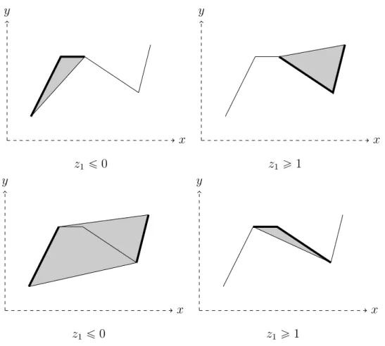
3-7 LP relaxation of formulation (3.8) (shaded) after (Left) down-branching 𝑧1 ď 0, and (Right) up-branching 𝑧1 ě 1. The quadrilaterals that are

feasible for each subproblem are crosshatched. . . 120

3-8 LP relaxation of formulation (3.9) (shaded) after (First row) down-branching 𝑧1 ď 0 or up-branching 𝑧1 ě 1; (Second row)

down-branching 𝑧1 ď 1or up-branching 𝑧1 ě 2; (Third row) down-branching

𝑧1 ď 2or up-branching 𝑧1 ě 3; or (Last row) down-branching 𝑧1 ď 3

or up-branching 𝑧1 ě 4. The quadrilaterals that are feasible for each

3-9 LP relaxation of embedding formulation for the annulus using the binary zig-zag encoding 𝐻ZZB

8 (shaded) after (Left) down-branching

𝑧1 ď 0, and (Right) up-branching 𝑧1 ě 1. The quadrilaterals that are

feasible for each subproblem are crosshatched. . . 122

4-1 The LP relaxation of an ideal formulation for (1.11) (e.g. Log/LogIB, Inc, or ZZI) projected onto p𝑥, 𝑦q-space. . . 130 4-2 The LP relaxation of the Inc formulation (4.3) projected onto p𝑥,

𝑦q-space, after (Top Left) down-branching 𝑧1 ď 0, (Top Right)

up-branching 𝑧1 ě 1; (Center Left) down-branching 𝑧2 ď 0, (Center

Right)up-branching 𝑧2 ě 1; (Bottom Left) down-branching 𝑧3 ď 0,

and (Bottom Right) up-branching 𝑧3 ě 1. . . 132

4-3 The Log formulation after (Left) down-branching 𝑧1 ď 0 and (Right)

up-branching 𝑧1 ě 1. . . 133

4-4 The LP relaxation of the ZZI formulation (4.2) projected onto p𝑥, 𝑦q-space, after (Top Center) down-branching 𝑧1 ď 0, (Bottom

Cen-ter) up-branching 𝑧1 ě 1, (Top Right) down-branching 𝑧1 ď 1, and

(Bottom Right)up-branching 𝑧1 ě 2. . . 134

4-5 PiecewiseLinearOpt code showing how to add univariate and bivariate piecewise linear functions to a JuMP model. . . 143

4-6 JuMP code for the cutting circle problem using PiecewiseLinearOpt. 145

5-1 Illustration of the branching scheme for the moment curve encoding 𝐻mc

7 . The original code relaxation in the 𝑧-space is shown in the dashed

region, and those for the two subproblems are shown in the darker shaded regions. The optimal solution for the original LP relaxation is depicted with a solid dot. We show the branching with a solution ˆ𝑧 that is fractional (Left), and one where ˆ𝑧 P Convp𝐻mc

7 qz𝐻7mc and yet

there is no valid variable branching disjunction to separate the point (Right). . . 165 5-2 The exotic two-dimensional encoding 𝐻ex

5-3 Branching scheme for the exotic encoding 𝐻mc

16 when the LP optimal

solution for the integer variables ˆ𝑧 has: (Left) ˆ𝑧1 fractional, (Center)

ˆ

𝑧1 P Z but ˆ𝑧2 R 𝑌 “ t ℎ2 | ℎ P 𝐻16mcu, and (Right) ˆ𝑧1 P Z, ˆ𝑧2 P 𝑌, and

yet ˆ𝑧 R 𝐻mc

16 . The relaxations for the two subproblems in each are the

two shaded regions in each picture. . . 168

5-4 A grid triangulation with 𝑑 “ 8 triangles. The nodes, or vertices for the triangles, are numbered. . . 173

5-5 The LP relaxation of the moment curve formulation (5.8) applied to the the piecewise linear function (1.11) projected onto p𝑥, 𝑦q-space, after (Top Left) branching on Ψ4p1, 1q, (Top Right) branching on

Ψ4p2, 4q; (Center Left) branching on Ψ4p1, 2q, (Center Right)

branch-ing on Ψ4p3, 4q; (Bottom Left) branching on Ψ4p1, 3q, and (Bottom

Right) branching on Ψ4p4, 4q. . . 175

5-6 The LP relaxation of the moment curve formulation (5.8) projected onto p𝑥, 𝑦q-space, after (Top Left) down-branching 𝑧1 ď 1, (Top

Right) up-branching 𝑧1 ě 2; (Center Left) down-branching 𝑧1 ď

2, (Center Right) up-branching 𝑧1 ě 3; (Bottom Left)

down-branching 𝑧1 ď 3, and (Bottom Right) up-branching 𝑧1 ě 4. . . 176

5-7 The LP relaxation of the very small SOS2 MIP-with-holes formulation (5.9) projected onto p𝑥, 𝑦q-space, after (Top Left) down-branching 𝑧1 ď ´1, (Top Right) up-branching 𝑧1 ě 0; (Center Left)

down-branching 𝑧1 ď 0, and (Center Right) up-branching 𝑧1 ě 1. . . 178

5-8 LP relaxation of the exotic formulation (5.11) (shaded) after (First row) down-branching 𝑧1 ď ´2 or up-branching 𝑧1 ě ´1; (Second

row) down-branching 𝑧1 ď ´1or up-branching 𝑧1 ě 0; (Third row)

down-branching 𝑧1 ď 0 or up-branching 𝑧1 ě 1; or (Last row)

down-branching 𝑧1 ď 1 or up-branching 𝑧1 ě 2. The quadrilaterals that are

B-1 The joining or splitting which transform a polygonal partition into one adhering to the conditions in Theorem 2 (before on Top, after on Bottom): (Left) splitting along an internal vertex, (Center) filling in a minimal infeasible set 𝑇 of cardinality three with Convp𝑇 q Ă Ω, and (Right)introducing an artificial vertex to remove a minimal infeasible set 𝑇 of cardinality three with Convp𝑇 q Ć Ω. . . 184

C-1 Feasible region in the p𝑥, 𝑦q-space for the Log formulation (C.2) after: (Left) down-branching 𝑧1 ď 0, and (Right) up-branching 𝑧1 ě 1. . . 189

C-2 Feasible region in the p𝑥, 𝑦q-space for the ZZI formulation (C.3) af-ter: (Top first column) down-branching on 𝑧1 ď 0, (Bottom first

column) up-branching on 𝑧1 ě 1; (Top second column)

down-branching on 𝑧1 ď 1, (Bottom second column) up-branching on

𝑧1 ě 2; (Top third column) down-branching on 𝑧1 ď 2, (Bottom

third column)up-branching on 𝑧1 ě 3; (Top fourth column)

down-branching on 𝑧1 ď 3, and (Bottom fourth column) up-branching on

List of Tables

1.1 Notation used throughout the paper. . . 49

4.1 Computational results for univariate transportation problems on small networks with non powers-of-two segments. . . 126

4.2 Computational results with Gurobi for univariate transportation prob-lems on small networks with non powers-of-two segments. . . 127

4.3 Computational results for univariate transportation problems on large networks with non powers-of-two segments. . . 127

4.4 Difficult univariate transportation problems on large networks with non powers-of-two segments. . . 127

4.5 Metrics for each possible branching decision on 𝑧1 for Inc, Log, and

ZZIapplied to (1.11). Notationally, 1 Ó means down-branching on the value 1 (i.e. 𝑧1 ď 1, and similarly 2 Ò implies up-branching on the

value 2 (i.e. 𝑧1 ě 2. . . 131

4.6 Computational results for bivariate transportation problems on grids of size “ 𝑑1 “ 𝑑2. . . 139

4.7 Computational results for transportation problems whose objective function is the sum of bivariate piecewise linear objective functions on grids of size 𝜅 “ 𝑑1 “ 𝑑2, when 𝜅 is not a power-of-two. . . 140

4.8 Comparison of bivariate piecewise-linear grid triangulation formula-tions using the 6-stencil approach (6S) against an optimal triangle se-lection formulation (Opt) on grids of size 𝜅 “ 𝑑1 “ 𝑑2. . . 141

C.1 Metrics for each possible branching decision on 𝑧1 for Log and ZZI

applied to (C.1). . . 189

D.1 Computational results with Gurobi for univariate transportation prob-lems on large networks with non powers-of-two segments. . . 191

D.2 Computational results with Gurobi for bivariate transportation prob-lems on grids of size 𝜅 “ 𝑑1 “ 𝑑2. . . 192

Chapter 1

Preliminaries.

The aim of this thesis is to develop new methods to solve difficult optimization prob-lems, efficiently. The class of “difficult” optimization problems we focus on are non-convex, and possibly discrete. Nonconvex optimization is difficult from a complexity perspective, even for restrictive subclasses such as nonconvex quadratic optimiza-tion [112]. Therefore, we mean “efficiently” in a practical sense, and we will endeavor to produce provably optimal solutions (or rigorous bounds on suboptimality) in a reasonable amount of time. At the end of this chapter, we will present a taxonomy of nonconvex structures that arise in a number of compelling applications. After this, we spend the rest of this thesis developing a number of advanced techniques to build good representations, or formulations, for them, and apply these techniques to produce substantial speed-ups over existing approaches.

1.1

Mixed-integer programming and formulations

Suppose that we have an optimization problem of the form min

𝑥,𝑦 𝑏 ¨ 𝑥 ` 𝑐 ¨ 𝑦 (1.1a)

s.t. 𝑥 P 𝐷 (1.1b)

where 𝑋 is a convex set, and 𝐷 is a nonconvex set that describes some portion of the feasible region.

In this context, it is well known that merely convexifying 𝐷 by replacing it with its convex hull (i.e. changing (1.1b) to 𝑥 P Convp𝐷q) is not sufficient for solving (1.1)1_.

Instead, we will add auxiliary variables 𝑤 and 𝑧 and craft a linear programming (LP) relaxation given by an inequality (outer) description as

𝑅 “ $ ’ ’ ’ ’ ’ ’ & ’ ’ ’ ’ ’ ’ % p𝑥, 𝑤, 𝑧q P R𝑛`𝑝`𝑟 ˇ ˇ ˇ ˇ ˇ ˇ ˇ ˇ ˇ ˇ ˇ ˇ 𝑙𝑥_{ď 𝑥 ď 𝑢}𝑥 𝑙𝑤 ď 𝑤 ď 𝑢𝑤 𝑙𝑧 _{ď 𝑧 ď 𝑢}𝑧 𝐴𝑥 ` 𝐵𝑤 ` 𝐶𝑧 ď 𝑑 , / / / / / / . / / / / / / -. (1.2)

We will say say that

𝐹 “ t p𝑥, 𝑦, 𝑧q P 𝑅 | 𝑧 P Z𝑟u (1.3)

is a mixed-integer programming (MIP) formulation for 𝐷 if 𝐷 “ Proj𝑥p𝐹 q

def

“ t 𝑥 | D𝑤, 𝑧 s.t. p𝑥, 𝑤, 𝑧q P 𝐹 u .

We call 𝑥 the original variables, 𝑤 the (optional) continuous auxiliary variables, and 𝑧 the integer variables of our formulation. An important subclass of formulations will be binary MIP formulations, where 𝑙𝑧

“ 0𝑟 and 𝑢𝑧 “ 1𝑟. Otherwise, we call 𝐹 a general integer MIP formulation.

We can use our formulation to solve the optimization problem (1.1) as min 𝑥,𝑦,𝑧,𝑤 𝑏 ¨ 𝑥 ` 𝑐 ¨ 𝑦 (1.4a) s.t. p𝑥, 𝑤, 𝑧q P 𝑅 (1.4b) p𝑥, 𝑦q P 𝑋 (1.4c) 𝑧 P Z𝑟. (1.4d) 1

As a simple example, take 𝑏 “ 𝑐 “ 1, 𝐷 “ t´1, 1u, and 𝑋 “ R2ě0. The optimal solution to (1.1) is p𝑥, 𝑦q “ p1, 0q with cost 1, while the convexified version has optimal solution p𝑥, 𝑦q “ p0, 0q with cost 0.

This is a mixed-integer programming problem, with a convex relaxation and non-convexity arising only from the integrality imposed on the 𝑧 variables. Of course, realistic optimization problems may contain a number of nonconvexities, meaning we will need to repeat this procedure.

Mixed-integer programming is surprisingly expressive class of optimization prob-lems, capable of modeling many complex problems of interest throughout opera-tions [38, 39, 90], analytics [18, 19], engineering [56, 60, 124], and robotics and con-trol [15,46, 47, 49,85, 103, 114], to name just a few. Moreover, there exist sophisti-cated algorithms–and corresponding high-quality software implementations–that can solve many problems of this form efficiently in practice [24,74]. For the remainder, we will focus on building formulations for nonconvex substructures like 𝐷 individually, and then composing them afterwards as in (1.4).

1.2

Disjunctive constraints

A central modeling primitive in mathematical optimization is the disjunctive con-straint: any feasible solution must satisfy at least one of some fixed, finite collection of alternatives. This type of constraint is general enough to capture structures as di-verse as boolean satisfiability, complementarity constraints, special-ordered sets, and (bounded) integrality. The special case of polyhedral disjunctive constraints corre-sponds to the form

𝑥 P 𝐷 def“

𝑑

ď

𝑖“1

𝑃𝑖, (1.5)

where we have that each alternative 𝑃𝑖

Ď R𝑛 is a polyhedron. We will make the following simplifying assumption on the structure of 𝐷.

Assumption 1. There are a finite number of alternatives 𝑃𝑖_{, and each is a rational,}

bounded polyhedron.

1.2.1

Combinatorial disjunctive constraints

We will spend much of this thesis focusing on a particular class of disjunctive con-straints that are both incredibly expressive and readily amenable to advanced formu-lation construction techniques. In particular, we will focus on disjunctive constraints where each alternative is a face of the standard simplex.

Definition 1. Take some finite set 𝑉 Ă R𝑛_{. A combinatorial disjunctive constraint}

(CDC) given by the family of sets 𝒯 “ p𝑇𝑖

Ď 𝑉 q𝑑𝑖“1 is a disjunctive constraint of the

form 𝜆 P CDCp𝒯 q“def 𝑑 ď 𝑖“1 𝑃 p𝑇𝑖q, where • suppp𝜆qdef

“ t 𝑣 P 𝑉 | 𝜆𝑣 ‰ 0 u is the set of nonzero components of 𝜆,

• ∆𝑉 def “ 𝜆 P R𝑉ě0 ˇ ˇ ř 𝑣P𝑉 𝜆𝑣 “ 1 (

is the standard simplex, and • 𝑃 p𝑇 q def

“ 𝜆 P ∆𝑉 ˇˇsuppp𝜆q Ď 𝑇 (

is the face that 𝑇 Ď 𝑉 induces on the stan-dard simplex.

We call 𝑉 the ground set for the constraint.

Although combinatorial disjunctive constraints can arise naturally as primitive constraints (see Chapters1.3.3and1.3.4), they also offer a principled way to construct formulations for arbitrary disjunctive constraints.

Due to the celebrated Minkowski-Weyl Theorem (e.g. [34, Corollary 3.14]), we can write each of our polyhedral alternatives 𝑃𝑖 _{as the convex combination of its}

extreme points 𝑇𝑖 _{“ extp𝑃}𝑖_q:

𝑃𝑖 “ Convp𝑇𝑖qdef“ # ÿ 𝑣P𝑇𝑖 𝜆𝑣𝑣 ˇ ˇ ˇ ˇ ˇ 𝜆 P ∆𝑇𝑖 + . (1.6)

for 𝑉 “ Ť𝑑 𝑖“1extp𝑃 𝑖_{q. Then (1.6) is equivalent to} 𝑃𝑖 “ # ÿ 𝑣P𝑉 𝜆𝑣𝑣 ˇ ˇ ˇ ˇ ˇ 𝜆 P 𝑃 p𝑇𝑖q + ,

where the constraint 𝜆 P 𝑃 p𝑇𝑖

q ensures that each new component of 𝜆 not corre-sponding to an extreme point of 𝑃𝑖 _{must be zero. If we take the family of sets}

𝒯 “ p𝑇𝑖

“ extp𝑃𝑖qq𝑑𝑖“1, then the combinatorial disjunctive constraint approach gives

us a way to formulate a disjunctive set as 𝐷 ” 𝑑 ď 𝑖“1 𝑃𝑖 “ # ÿ 𝑣P𝑉 𝜆𝑣𝑣 ˇ ˇ ˇ ˇ ˇ 𝜆 P CDCp𝒯 q + . (1.7)

Note that all the nonconvexity of the set 𝐷 has now been encapsulated in CDCp𝒯 q. Therefore, we can focus on formulating CDCp𝒯 q, which will often be much simpler than formulating 𝐷 directly, and then easily construct a formulation for 𝐷 by ap-plying a linear transformation to the 𝜆 variables. The disjunctive constraints are combinatorial since they rely on the shared structure of the extreme points among the different alternatives, captured in the family of sets 𝒯 .

Moreover, it is straightforward to extend the combinatorial disjunctive constraint approach to accommodate unbounded alternatives (provided standard representabil-ity conditions are satisfied [72] [130, Proposition 11.2]) as

𝐷 “ # ÿ 𝑣P𝑉 𝜆𝑣𝑣 ` ÿ 𝑟P𝑅 𝜇𝑟𝑟 ˇ ˇ ˇ ˇ ˇ 𝜆 P CDCp𝒯 q, 𝜇 P R𝑅ě0 + , (1.8)

where 𝑅 is the shared set of extreme rays for each of the 𝑃𝑖_{. We offer this as}

justification for Assumption1, as formulating the unbounded case is a straightforward extension.

Much of the work of this thesis will be in deriving formulations for CDCp𝒯 q, given a particular family of sets 𝒯 over some ground set 𝑉 . We make the following assumptions about 𝒯 that are without loss of generality.

• The constraint is disjunctive: |𝒯 | ą 1.

• Each alternative is nonempty: 𝑇 ‰ H for all 𝑇 P 𝒯 .

• 𝒯 is irredundant: there do not exist distinct 𝑇, 𝑇1 _{P 𝒯} such that 𝑇 Ď 𝑇1.

• 𝒯 covers the ground set: Ť𝑑 𝑖“1𝑇

𝑖

“ 𝑉.

We will say that a set 𝑇 Ď 𝑉 is a feasible set with respect to (w.r.t.) CDCp𝒯 q if 𝑃 p𝑇 q Ď CDCp𝒯 q (equivalently, if 𝑇 Ď 𝑇1 for some 𝑇1

P 𝒯) and that it is an infeasible set otherwise. Notationally, given the family of sets 𝒯 “ p𝑇𝑖 _{Ď 𝑉 q}𝑑

𝑖“1, we

will find it useful to refer to the corresponding family of faces of the standard simplex 𝒫p𝒯 qdef“ p𝑃 p𝑇𝑖qq𝑑_𝑖“1, which are the alternatives of the disjunctive constraint which we ultimately will formulate.

1.2.2

Combinatorial disjunctive constraints and data

indepen-dence

One distinct advantage of the combinatorial disjunctive constraint approach is that the formulation (1.7) allows us to divorce the problem-specific data (i.e. the values 𝑣 P 𝑉) from the underlying combinatorial structure in 𝒯 . As such, we can construct a single, strong formulation for a given structure CDCp𝒯 q, and this formulation will remain valid for transformations of the data, so long as this transformation suffi-ciently preserves the combinatorial structure of CDCp𝒯 q. For instance, if we formu-late Ť𝑑

𝑖“1𝑃𝑖 via its corresponding combinatorial disjunctive constraint CDCp𝒯 q, and

then change the data to produce a related disjunctive constraint Ť𝑑 𝑖“1𝑃ˆ

𝑖_{, a sufficient}

condition for our formulation of CDCp𝒯 q to yield a valid formulation for Ť𝑑

𝑖“1𝑃ˆ𝑖 is

the existence of a bijection 𝜋 : 𝑉 Ñ ˆ𝑉 (with 𝑉 “ Ť𝑑

𝑖“1extp𝑃 𝑖 qand ˆ𝑉 “ Ť𝑑_𝑖“1extp ˆ𝑃𝑖q) such that 𝑣 P extp𝑃𝑖q ðñ 𝜋p𝑣q P extp ˆ𝑃𝑖q @𝑖 PJ𝑑K, 𝑣 P 𝑉 , (1.9) where J𝑑K def

“ t1, . . . , 𝑑u. In this way, we can construct a single small, strong formula-tion for CDCp𝒯 q, and use it repeatedly for many different “combinatorially equivalent” instances of the same constraint.

We note that one subtle disadvantage of this data-agnostic approach is that, even if condition (1.9) is satisfied, the resulting formulation for Ť𝑑

𝑖“1𝑃ˆ𝑖 may be larger

than necessary. An extreme manifestation of this would be when the new polyhedra p ˆ𝑃𝑖_q𝑑

𝑖“1 are such that ˆ𝑃𝑖 Ď ˆ𝑃1 for all 𝑖 P J𝑑K. In this case, Ť

𝑑

𝑖“1𝑃ˆ𝑖 “ ˆ𝑃1 and

the constraint is no longer truly disjunctive, meaning it can be modeled directly as a LP. Less pathological cases could occur where some subset of the disjunctive sets become redundant after changing the problem data. However, we note that in many of the applications considered in this work, the combinatorial representation leads to redundancy of this form only in rare pathological cases (this is true of the constraints in Chapter1.3.2, for example). In other cases we will take care to consider, for example, the geometric structure of the data before constructing the disjunctive constraint (e.g. our results in Chapter 2.3.3).

1.3

Motivating problems

We now present constraints, arising in a number of application areas across engineer-ing, robotics, power systems, and machine learnengineer-ing, that we will return to throughout. The first seven will fall neatly into the combinatorial disjunctive constraint frame-work. However, the last does not, and we will explore other techniques to construct strong formulations for it in Chapter 4.

1.3.1

Modeling discrete alternatives

The special-ordered set (SOS) constraints introduced by Beale and Tomlin [13] are a classical family of constraints with numerous applications throughout operations research. The SOS constraint of type 1 (SOS1) is given by the family of sets 𝒯SOS1

𝑁

def

“ pt𝑖uq𝑁_𝑣“1, and can be used to model discrete alternatives: given 𝑁 distinct points t𝑣𝑖u𝑁𝑖“1Ă R𝑛,

𝑥 P t𝑣𝑖u𝑁𝑖“1ðñ 𝑥 “ 𝑁

ÿ

𝑖“1

Notationally, we will refer to the SOS1 constraint on 𝑁 components (i.e. given by 𝒯SOS1

𝑁 with ground set 𝑉 “J𝑁 K) as SOS1(𝑁 ). In the following subsections, we will present other types of SOS constraints.

1.3.2

Piecewise linear functions

Consider an optimization problem of the form min𝑥PΩ𝑓 p𝑥q, where Ω Ď R𝑛 and 𝑓 :

Ω Ď R𝑛

Ñ R is a piecewise linear function. That is, 𝑓 can be described by a partition of the domain Ω into a finite family t𝐶𝑖_u𝑑

𝑖“1 of polyhedral pieces, where for each piece

𝐶𝑖 there is an affine function 𝑓𝑖 : 𝐶𝑖 Ñ R where 𝑓 p𝑥q “ 𝑓𝑖p𝑥q for each 𝑥 P 𝐶𝑖. In the same vein, we may consider an optimization problem where the feasible region is (partially) defined by a constraint of the form 𝑓p𝑥q ď 0, where 𝑓 is piecewise linear.

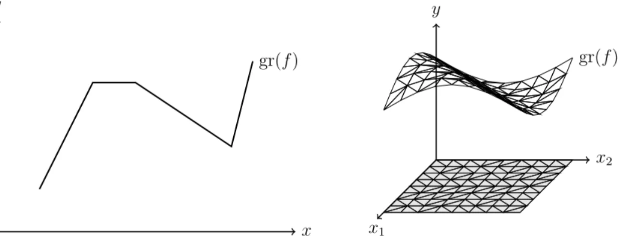
𝑥 𝑦 grp𝑓 q 𝑥1 𝑥2 𝑦 grp𝑓 q

Figure 1-1: (Left) A univariate piecewise linear function, and (Right) a bivariate piecewise linear function with a grid triangulated domain.

The potential applications for this class of optimization problems are legion. Piece-wise linear functions arise naturally throughout operations [38,39, 90] and engineer-ing [56, 60, 124]. They are a natural choice for approximating nonlinear functions, as they often lead to optimization problems that are easier to solve than the original problem [16, 17, 28, 58, 82, 106, 104]. For example, there has been recently been significant interest in using piecewise linear functions to approximate complex non-linearities arising gas network optimization problems [32, 33, 101, 97, 105, 125]; see [80] for a recent book on the subject.

If the function 𝑓 happens to be convex, it is possible to reformulate our opti-mization problem into an equivalent LP problem (provided that Ω is polyhedral) However, if 𝑓 is nonconvex, this problem is NP-hard in general [78]. A number of specialized algorithms for solving piecewise linear optimization problems have been proposed over the years [13, 45, 44, 78, 128]. Instead, we will focus on MIP for-mulations for piecewise linear function, an active and fruitful area of research for decades [10, 38, 41, 42,72, 71, 77,89, 96, 99, 111,123,135,133,137].

We consider continuous2 piecewise linear functions 𝑓 : Ω Ñ R, where Ω Ă R𝑛

is bounded. We will describe 𝑓 in terms of the domain pieces t𝐶𝑖

Ď Ωu𝑑𝑖“1 and the

corresponding affine functions t𝑓𝑖_u𝑑

𝑖“1. We assume that the pieces cover the domain

Ω, and that their relative interiors do not overlap. Furthermore, we assume that our function 𝑓 is non-separable and cannot be decomposed as the sum of lower-dimensional piecewise linear functions. This is without loss of generality, as if such a decomposition exists, we could apply our formulation techniques to the individual pieces separately. Finally, we will spend a substantial amount time on the regime where the dimension 𝑛 of the domain is relatively small: when 𝑓 is either univariate (𝑛 “ 1) or bivariate (𝑛 “ 2) with a grid triangulated domain; see Figure 1-1 for an illustrative example of each.

In order to solve an optimization problem containing 𝑓, we will construct a for-mulation for its graph

grp𝑓 ; Ωq“ t p𝑥, 𝑓 p𝑥qq | 𝑥 P Ω u .def We can write this graph disjunctively as grp𝑓q “ Ť𝑑

𝑖“1𝑃

𝑖_{, where each alternative 𝑃}𝑖

“ t p𝑥, 𝑓𝑖p𝑥qq | 𝑥 P 𝐶𝑖 uis a segment of the graph. We can then take 𝒯 “ pextp𝐶𝑖qq𝑑𝑖“1,

formulate CDCp𝒯 q, and express the graph as grp𝑓 q “ # ÿ 𝑣P𝑉 𝜆𝑣p𝑣, 𝑓 p𝑣qq ˇ ˇ ˇ ˇ ˇ 𝜆 P CDCp𝒯 q + , (1.10)

where we will use the notation grp𝑓q ” grp𝑓; Ωq when Ω is clear from context.

2_{The results to follow can potentially be extended to discontinuous piecewise linear functions by} working instead with the epigraph of 𝑓 ; we point the interested reader to [133,134].

Univariate piecewise linear functions

For univariate piecewise linear functions (i.e. Ω Ă R), the corresponding combina-torial disjunctive constraint has a particularly nice structure. The domain partition will consist of 𝑑 adjacent intervals 𝐶𝑖

“ r𝜏𝑖, 𝜏𝑖`1s, given by 𝑁 ” 𝑑 ` 1 breakpoints 𝜏1 _{ă 𝜏}2 _{ă ¨ ¨ ¨ ă 𝜏}𝑁 that we presume are distinct. In particular, the family of sets will

be equivalent to the special-ordered set of type 2 (SOS2) constraint, which is defined as 𝒯SOS2

𝑑

def

“ pt𝑖, 𝑖 ` 1uq𝑑<sub>𝑖“1</sub>. In words, the constraint 𝜆 P CDCp𝒯<sub>𝑑</sub>SOS2qrequires that at most two components of 𝜆 may be nonzero, and that these nonzero components must be consecutive in the ordering on 𝑉 “ J𝑁 K. We will refer to the SOS2 constraint on 𝑁 ” 𝑑 ` 1 components as SOS2(𝑁).

As long as the ordering of the breakpoints is preserved, it is easy to see that condition (1.9) will be satisfied for any transformations of the problem data. Fur-thermore, the only case in which knowledge of the specific data tp𝜏𝑖_{, 𝑓 p𝜏}𝑖_qqu𝑑

𝑖“1 allows

the simplification of the original disjunctive representation of grp𝑓q is when 𝑓 is affine in on two adjacent intervals, e.g. affine over r𝜏𝑖_{, 𝜏}𝑖`2_{s for some 𝑖 P}

J𝑑 ´ 1K. There-fore, the potential disadvantage of disregarding the specific data when formulating the constraint occurs only in rare pathological cases which are easy to detect.

Example 1 (A univariate piecewise linear function). Consider the univariate piece-wise linear function 𝑓 : r0, 4s Ñ R. We decompose the domain into the four pieces 𝐶1 “ r0, 1s, 𝐶2 “ r1, 2s, 𝐶3 “ r2, 3s, and 𝐶4 “ r3, 4s, and describe the function as

𝑥 P 𝐶1 ùñ 𝑓 p𝑥q “ 4𝑥, 𝑥 P 𝐶2 ùñ 𝑓 p𝑥q “ 3𝑥 ` 1, (1.11a)

𝑥 P 𝐶3 ùñ 𝑓 p𝑥q “ 2𝑥 ` 3, 𝑥 P 𝐶4 ùñ 𝑓 p𝑥q “ 𝑥 ` 6. (1.11b)

The graph of the piecewise linear function is then grp𝑓 q “ p𝑥, 4𝑥qˇˇ𝑥 P 𝐶1 ( Y p𝑥, 3𝑥 ` 1qˇˇ𝑥 P 𝐶2 ( Y p𝑥, 2𝑥 ` 3qˇˇ𝑥 P 𝐶3 ( Y p𝑥, 𝑥 ` 6qˇˇ𝑥 P 𝐶4( .

Moreover, the function has 𝑑 “ 4 segments, and is given by the breakpoints t𝜏𝑖

p𝑖 ´ 1qu4𝑖“1. Taking, without loss of generality (w.l.o.g.), the ground set as 𝑉 “ J5K, we can observe that

p𝑥, 𝑦q P grp𝑓 q ðñ p𝑥, 𝑦q “ ÿ

𝑣P𝑉

p𝜏𝑣, 𝑓 p𝜏𝑣qq𝜆𝑣 for some 𝜆 P CDCp𝒯4SOS2q.

Bivariate piecewise linear functions and grid triangulations

Consider a (potentially nonconvex) region Ω Ă R2 in the plane. We would like to

model a (also potentially nonconvex) piecewise linear function 𝑓 with domain over Ω; see Figure 1-1 for an illustration. If we take t𝐶𝑖_u𝑑

𝑖“1 as a partition of the domain Ω,

along with the family of sets 𝒯 “ pextp𝐶𝑖

qq𝑑𝑖“1with ground set 𝑉 “ Ť 𝑑

𝑖“1extp𝐶 𝑖_{q, we}

can model the piecewise linear function via the graph representation (1.10).

Example 2(A bivariate piecewise linear function). Take the bivariate piecewise linear function 𝑓 : r0, 1s2

Ñ R given by the domain partition 𝐶1 “ t 𝑥 P r0, 1s2 | 𝑥1 ě 𝑥2u

and 𝐶2

“ t 𝑥 P r0, 1s2 | 𝑥1 ď 𝑥2u, and

𝑥 P 𝐶1 ùñ 𝑓 p𝑥q “ ´𝑥1` 3𝑥2` 1, 𝑥 P 𝐶2 ùñ 𝑓 p𝑥q “ 𝑥1` 𝑥2` 1. (1.12)

See the left side of Figure 1-3 for an illustration. The corresponding graph is grp𝑓 q “ p𝑥, ´𝑥1` 3𝑥2` 1q ˇ ˇ𝑥 P 𝐶1 ( Y p𝑥, 𝑥1` 𝑥2` 1q ˇ ˇ𝑥 P 𝐶2( . Furthermore, 𝑉 “ t0, 1u2_{, and with 𝒯 “ ptp0, 0q, p1, 0q, p1, 1qu, tp0, 0q, p0, 1q, p1, 1quq,}

p𝑥, 𝑦q P grp𝑓 q ðñ p𝑥, 𝑦q “ ÿ

𝑣P𝑉

p𝑣, 𝑓 p𝑣qq𝜆𝑣 for some 𝜆 P CDCp𝒯 q.

An important special case we will focus on occurs when the function 𝑓 is affine over a grid triangulation, as in Figure 1-1 and Example 2. Consider a rectangular region in the plane Ω “ r1, 𝑁1s ˆ r1, 𝑁2s where along each axis we apply a discretization

with 𝑑1 “ 𝑁1 ´ 1 and 𝑑2 “ 𝑁2 ´ 1 breakpoints, respectively. This leads to a set of

a family of sets 𝒯 where:

• Each 𝑇 P 𝒯 is a triangle: |𝑇 | “ 3.

• 𝒯 partitions Ω: Ť𝑇 P𝒯 Convp𝑇 q “ Ωand intpConvp𝑇 qq X intpConvp𝑇1qq “ Hfor

each distinct 𝑇, 𝑇1

P 𝒯 (where intp𝑆q is the interior of set 𝑆). • 𝒯 is on a regular grid: ||𝑣 ´ 𝑤||8 ď 1 for each 𝑇 P 𝒯 and 𝑣, 𝑤 P 𝑇 .

Grid triangulations can possess a very rich and irregular combinatorial structure; see Figure 1-2, for three different triangulations with 𝑑1 “ 𝑑2 “ 2. Note that any

formulation constructed for a given grid triangulation can be readily applied to any other grid triangulation obtained by shifting the grid points in the plane, so long as the resulting triangulation is strongly isomorphic to, or compatible with, the original triangulation [3]. In particular, our choice of ground set 𝑉 “ t1, . . . , 𝑁1uˆt1, . . . , 𝑁2u

is without loss of generality, and we can readily adapt our formulations for grids with shifts or unequal interval lengths.

Figure 1-2: Three grid triangulations of Ω “ r1, 3s ˆ r1, 3s: (Left) the Union Jack (J1) [127], (Center) the K1 [84], and (Right) a more idiosyncratic triangulation.

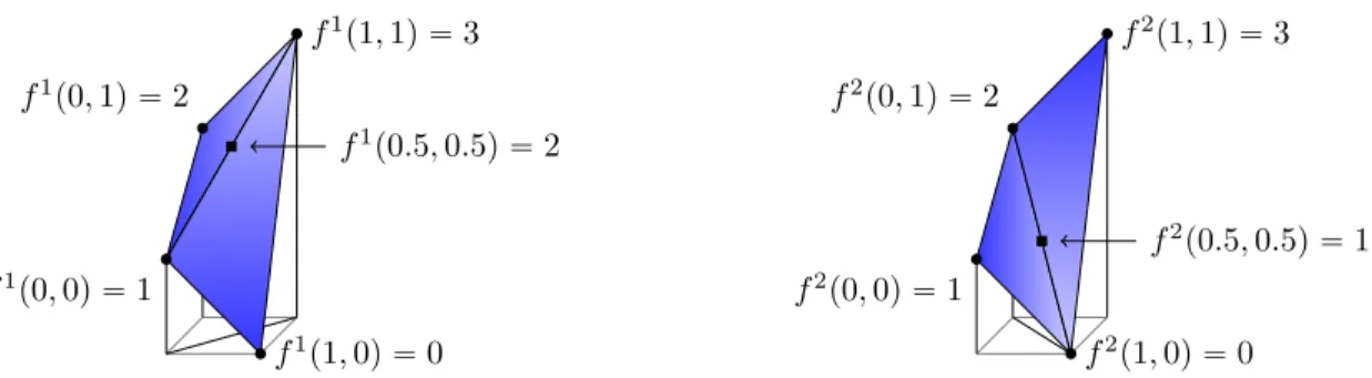
Finally, we note that the choice of triangulation is important, as it materially affects the values that the corresponding piecewise linear function takes. This is in sharp contrast to the univariate case, where the function is completely determined by the breakpoints and the value the function takes at those points. In Figure 1-3 we see a simple example of this, where two different triangulations lead to two bivariate functions which coincide at the corner points 𝑉 , but differ substantially in the interior of the domain.

𝑓1 p0, 0q “ 1 𝑓1p1, 0q “ 0 𝑓1 p0, 1q “ 2 𝑓1p1, 1q “ 3 𝑓1 p0.5, 0.5q “ 2 𝑓2 p0, 0q “ 1 𝑓2p1, 0q “ 0 𝑓2 p0, 1q “ 2 𝑓2p1, 1q “ 3 𝑓2 p0.5, 0.5q “ 1

Figure 1-3: Two bivariate functions over 𝐷 “ r0, 1s2 _{that match on the gridpoints,}

but differ on the interior of 𝐷.

Higher-dimensional piecewise linear functions Beyond univariate and bivari-ate piecewise linear functions, it is also possible to define piecewise linear functions over higher-dimensional grid triangulations. Given a 𝜂-dimensional piecewise linear function 𝑓 : Ω Ñ R, where Ω Ă R𝜂 _{is a hyperrectangular domain. As was the}

case with univariate and bivariate functions, assume that Ω “ ś𝜂

𝑖“1r1, 𝑁𝑖s and take

the regularly gridded ground set 𝑉 “ ś𝜂

𝑖“1J𝑁𝑖K, along with a 𝜂-dimensional grid triangulation given by the family of sets 𝒯 , where

• Each 𝑇 P 𝒯 is a simplex: |𝑇 | “ 𝜂 ` 1.

• 𝒯 partitions Ω: Ť𝑇 P𝒯 Convp𝑇 q “ Ωand intpConvp𝑇 qq X intpConvp𝑇 1

qq “ Hfor each distinct 𝑇, 𝑇1 _{P 𝒯}.

• 𝒯 is on a regular grid: ||𝑣 ´ 𝑤||8 ď 1 for each 𝑇 P 𝒯 and 𝑣, 𝑤 P 𝑇 .

Note that this definition is a generalization of that given in the previous subsection for grid triangulations in the plane (𝜂 “ 2). The combinatorial structure for higher-dimensional grid triangulations is even more complex than in the two-higher-dimensional case: for example, different choices of triangulation for a single hypercube (e.g. t0, 1u𝜂) can have different numbers of triangles [98, 127]. One possible choice is the standard triangulation for t0, 1u𝜂_{, given by the family}

𝑇𝜋 “ 𝑥 P t0, 1u𝜂 ˇˇ𝑥_𝜋p1qď 𝑥_𝜋p2q ď ¨ ¨ ¨ ď 𝑥_𝜋p𝜂q (

(1.13) for each permutation 𝜋 of J𝜂K.

High-dimensional piecewise linear functions arise in a number of important opti-mization contexts (see, for example, Chapter 1.3.8), but unless 𝜂 is very small they quickly strain the practicality of the combinatorial disjunctive constraint approach. This is because the cardinality of the ground set 𝑉 will grow exponentially in 𝜂, and as the formulation (1.7) requires an auxiliary variable 𝜆𝑣 for each element 𝑣 P 𝑉 , this

overhead can quickly become overwhelming.

1.3.3

The SOS𝑘 constraint

In addition to the SOS1 and SOS2 constraints we have described above, we can generalize the class of constraints to special-ordered sets of type 𝑘 (SOS𝑘), where at most 𝑘 consecutive components of 𝜆 may be nonzero at once. In particular, if 𝑉 “ J𝑁 K, we have 𝒯

SOS 𝑁,𝑘

def

“ pt𝜏, 𝜏 ` 1, . . . , 𝜏 ` 𝑘 ´ 1uq𝑁 ´𝑘`1_𝑖“1 . This constraint may arise, for example, in chemical process scheduling problems, where an activated machine may only be on for 𝑘 consecutive time units and must produce a fixed quantity during that period [52,83]. We will refer to the SOS𝑘 constraint on 𝑁 components as SOS𝑘(𝑁).

1.3.4

Cardinality constraints

An extremely common constraint in optimization is the cardinality constraint of de-gree ℓ, where at most ℓ components of 𝜆 may be nonzero. This corresponds to the family of sets 𝒯card

𝑁,ℓ

def

“ p𝑇 Ď 𝑉 | |𝑇 | “ ℓq, where we presume that 𝑉 “ J𝑁 K for simplicity. A particularly compelling application of the cardinality constraint is in portfolio optimization [20, 22, 30, 132], where it is often advantageous to limit the number of investments to some fixed number ℓ to minimize transaction costs, or to allow differentiation from the performance of the market as a whole.

1.3.5

Discretizations of multilinear functions

Consider a multilinear function 𝑓p𝑥1, . . . , 𝑥𝜂q “

ś𝜂

𝑖“1𝑥𝑖 defined over some

hyperrect-angular domain Ω “ r𝑙, 𝑢s Ă R𝜂. This function appears often in optimization models

global optimality in practice [6, 115, 136]. As a result, computational techniques will often “relax” the graph of the function grp𝑓q with a convex outer approximation, which is easier to optimize over [119].

For the bilinear case (𝜂 “ 2), the well-known McCormick envelope [102] describes the convex hull of grp𝑓q. Although traditionally stated in an inequality description, we may equivalently describe the convex hull via its four extreme points, which are readily available in closed form. For higher-dimensional multilinear functions, the convex hull has 2𝜂 extreme points, and can be constructed in a similar manner (e.g.

see equation (3) in [95] and the associated references).

Misener et al. [104,106] propose a computational technique for optimizing prob-lems with bilinear terms where, instead of modeling the graph over a single region Ω “ r𝑙, 𝑢s Ă R2, they discretize the region in a regular fashion and apply the Mc-Cormick envelope to each subregion. They model this constraint as a union of poly-hedra, where each subregion enjoys a tighter relaxation of the bilinear term. Addi-tionally, they propose a logarithmically-sized formulation for the union. However, it is not ideal (see Appendix A), it only applies for bilinear terms (𝜂 “ 2), and it is specialized for a particular type of discretization (namely, only discretizing along one component 𝑥1, and with constant discretization widths).

For a more general setting, we have that the extreme points of the convex hull of the graph Convpgrp𝑓qq are given by t p𝑥, 𝑓p𝑥qq | 𝑥 P extpΩq u [95, equation (3)], where it is easy to see that extpΩq “ ś𝜂

𝑖“1t𝑙𝑖, 𝑢𝑖u. Consider a grid imposed on

r𝑙, 𝑢s Ă R𝜂; that is, along each component 𝑖 P J𝜂K, we partition r𝑙𝑖, 𝑢𝑖s along the points 𝑙𝑖 ” 𝜏1𝑖 ă 𝜏2𝑖 ă ¨ ¨ ¨ ă 𝜏𝑑𝑖𝑖 ă 𝜏 𝑖 𝑑𝑖`1 ” 𝑢𝑖. This yields ś 𝜂 𝑖“1𝑑𝑖 subregions; denote them by Rdef “ 𝑅𝑘“ś𝜂<sub>𝑖“1</sub>r𝜏𝑘𝑖𝑖, 𝜏 𝑖 𝑘𝑖`1s ˇ ˇ𝑘 P ś𝜂 𝑖“1J𝑑𝑖K ( .

We can then take the polyhedral partition of Ω given by Φ𝑅def

“ Convpgrp𝑓 ; 𝑅qqfor each subregion 𝑅, the sets as 𝒯 “ `extpΦ𝑅

q˘_𝑅PR, and the ground set as 𝑉 “ Ťt𝑇 P 𝒯 u. In particular, we have that 𝑉 “ ś𝜂

𝑖“1t𝜏1𝑖, . . . , 𝜏𝑁𝑖𝑖u, where 𝑁𝑖 “ 𝑑𝑖` 1 for each 𝑖.

Analogously to the notational simplification we took with grid triangulations, for the remainder we will take 𝑉 “ ś𝜂

𝑖“1J𝑁𝑖K and 𝒯 “ p ś𝜂

𝑖“1t𝑘𝑖, 𝑘𝑖` 1u | 𝑘 P

ś𝜂

𝑖“1J𝑑𝑖Kq. We also note that condition (1.9) is satisfied as long as the ordering of the discretization

B

A

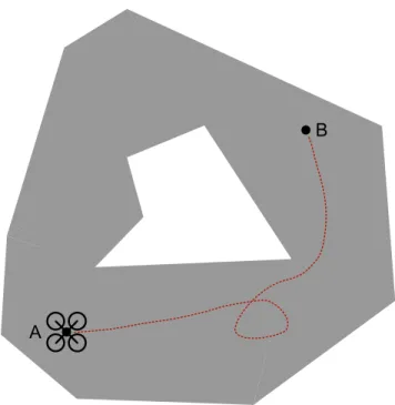
Figure 1-4: A trajectory for a UAV which avoids an obstacle in the center of the domain.

is respected along each dimension.

1.3.6

Obstacle avoidance constraints

Consider an unmanned aerial vehicle (UAV) which you would like to navigate through an area with fixed obstacles. At any given time, you wish to impose the constraint that the location of the vehicle 𝑥 P R2 _{must lie in some (nonconvex) region Ω Ă R}2_,

which is some (bounded) subset the plane, with any obstacles in the area removed. MIP formulations of this constraint has received interest as a useful primitive for path planning problems [15, 47, 103, 114].

We may model 𝑥 P Ω by partitioning the region Ω with polyhedra such that Ω “ Ť𝑑

𝑖“1𝑃

𝑖_{. Traditional approaches to modeling constraints (1.5) of this form use a linear}

inequality description for each of the polyhedra 𝑃𝑖 and construct a corresponding

big-𝑀 formulation [113, 114], which will not be strong, in general. However, it is clear that we may also apply our combinatorial disjunctive constraint approach to construct formulations for obstacle avoidance constraints.

1.3.7

Annulus constraints

An annulus is a set in the plane 𝒜 “ 𝑥 P R2 ˇ

ˇ𝑆 ď ||𝑥||₂ ď 𝑆 (

for constants 𝑆, 𝑆 P Rě0; see the left side of Figure 1-5 for an illustration. A constraint of the form 𝑥 P 𝒜

might arise when modeling a complex number 𝑧 “ 𝑥1 ` 𝑥2i, as 𝑥 P 𝒜 bounds the

magnitude of 𝑧 as 𝑆 ď |𝑧| ď 𝑆. Such constraints arise in power systems optimization: for example, in the “rectangular formulation” [81] and the second-order cone reformu-lation [69,91] of the optimal power flow problem and its voltage stability-constrained variant [40], and the reactive power dispatch problem [53]. Another application is footstep planning in robotics [46,85], where we wish to model an angle 𝜃 trigonomet-rically via 𝑥 “ pcosp𝜃q, sinp𝜃qq. This can be accomplished by imposing the identity 𝑥2

1` 𝑥22 “ 1, which corresponds to taking 𝑆 “ 𝑆 “ 1.

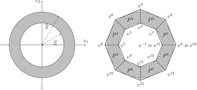
𝑥2 𝑥1 𝑆 𝑆 𝑃1 𝑃2 𝑃3 𝑃4 𝑃5 𝑃6 _𝑃7 𝑃8 𝑣´1 ” 𝑣15 𝑣0 ” 𝑣16 𝑣1 𝑣2 𝑣3 𝑣4 𝑣5 𝑣6 𝑣7 𝑣8 𝑣9 𝑣10 𝑣11 𝑣12 𝑣13 𝑣14

Figure 1-5: (Left) The annulus 𝒜 and (Right) its corresponding quadrilateral re-laxation ˆ𝒜 given by (1.14) with 𝑑 “ 8.

When 0 ă 𝑆 ď 𝑆, 𝒜 is a nonconvex set. Moreover, the annulus is not mixed-integer convex representable [93,94]: that is, there do not exist mixed-integer formulations for the annulus even if we allow the relaxation 𝑅 in formulation (1.3) to be an arbitrary convex set.

where each 𝑃𝑖 “ Conv ´ 𝑣2𝑖`𝑠´4(4 𝑠“1 ¯ @𝑖 P_J𝑑K (1.14)

is a quadrilateral based on the breakpoints 𝑣2𝑖´1 “ ˆ 𝑆 cosˆ 2𝜋𝑖 𝑑 ˙ , 𝑆 sinˆ 2𝜋𝑖 𝑑 ˙˙ @𝑖 P J𝑑K 𝑣2𝑖 “ ˆ 𝑆 sec ´𝜋 𝑑 ¯ cosˆ 2𝜋𝑖 𝑑 ˙ , 𝑆 sec ´𝜋 𝑑 ¯ sinˆ 2𝜋𝑖 𝑑 ˙˙ @𝑖 P J𝑑K,

where, for notational simplicity, we take 𝑣0 _{” 𝑣}2𝑑 and 𝑣´1 _{” 𝑣}2𝑑´1. We can in turn

represent this disjunctive relaxation through the combinatorial disjunctive constraint given by the family 𝒯ann

𝑑

def

“ pt2𝑖 ` 𝑠 ´ 4u4𝑠“1q𝑑𝑖“1. See the right side of Figure 1-5 for

an illustration.

1.3.8

Optimizing over trained neural networks

Since the turn of the millenia, deep learning has received an explosion of interest due to its successful application to a number of difficult problems in areas such as speech recognition and image classification [59, 87]. More recently, it has been recognized that trained feedforward neural networks with standard activation units are noth-ing more than high-dimensional (nonconvex) piecewise linear functions, and can be modeled using MIP. Indeed, a string of recent research has applied this observation to tasks such as verification, planning, and control [5, 31, 50, 121, 126, 138]. In this thesis, we will focus on neural networks that are built by composing a number of “rectified linear” (ReLu) activation units of the form

𝑓ReLup𝑥qdef“ maxt0, 𝑥u

with affine mappings 𝑤 ¨ 𝑥 ` 𝑏 which are learned during the training procedure. In particular, we will formulate the set resulting from composing an affine mapping with

a single ReLu unit:

ReLudef“ p𝑥, 𝑓ReLup𝑤 ¨ 𝑥 ` 𝑏qq ˇˇ𝐿 ď 𝑥 ď 𝑈 ( .

As we observed in Chapter 1.3.2, the combinatorial disjunctive constraint approach does not lend itself well to high dimensional piecewise linear functions of this form, as the ground set 𝑉 can grow exponentially in 𝜂. Therefore, in Chapter 4.4 we will strive to produce strong formulations through a different approach, though we will have to sacrifice formulation size as a result.

As an extension, we will also consider sets representing the composition of two layers with multiple nonlinear activation units applied to the same inputs, but with different affine mappings:

$ ’ ’ ’ & ’ ’ ’ % p𝑥, 𝑦1, . . . , 𝑦𝑑, ˜𝑦q ˇ ˇ ˇ ˇ ˇ ˇ ˇ ˇ ˇ 𝐿 ď 𝑥 ď 𝑈 𝑦𝑖 “ 𝑓ReLup𝑤𝑖¨ 𝑥 ` 𝑏𝑖q @𝑖 PJ𝑑K ˜ 𝑦 “ 𝑓ReLu p ˜𝑤 ¨ p𝑦1<sub>, . . . , 𝑦</sub>𝑑<sub>q ` ˜𝑏q</sub> , / / / . / / / -.

1.4

Assessing the quality of MIP formulations

Throughout this thesis, we will be interested in ways of understanding, both quantita-tively and qualitaquantita-tively, when we can expect a given MIP formulation to perform well in practice. We will focus on three measures of formulation quality, which empirically tend to correlate very strongly with computational performance [34, 130, 139].

1.4.1

Strength

First, we desire formulations whose LP relaxations are as tight as possible. The reason for this is simple: using a branch-and-bound-based approach, we rely on this LP relaxation to produce good dual bounds on the optimal objective value, which we in turn use to prune as much of the search tree as possible. Therefore, we would like to produce a relaxation that is as tight as possible (without losing validity), since this will produce dual bounds that are as strong as possible.

There are two standard notions of formulation strength, that consider either the original variables 𝑥, or the integer variables 𝑧.

Definition 2. Take a formulation 𝐹 “ t p𝑥, 𝑤, 𝑧q P 𝑅 | 𝑧 P Z𝑟

u for 𝐷 Ă R𝑛, given by the LP relaxation 𝑅. We say the formulation is:

• sharp if Proj𝑥p𝑅q “ Convp𝐷q.

• ideal if Proj𝑧pextp𝑅qq Ď Z𝑟.

Sharp formulations are desirable as they offer the tightest possible convex relax-ation in the 𝑥-space, and so in turn give the strongest possible dual bounds; see Figure 1-6 for an illustration. Ideal formulations are desirable since, if you solve the optimization problem over the corresponding relaxation, you are guaranteed the ex-istence of an optimal solution that is integer feasible w.r.t. (1.4d), and optimal for the original MIP problem.

𝑥 𝑦

𝑥 𝑦

Figure 1-6: The relaxations (gray region) for two different formulations of a nonconvex set (solid lines), corresponding a univariate piecewise linear function. (Left) One is not sharp, while (Right) the second is sharp. If we solve the relaxted optimization problem minp𝑥,𝑦qP𝑅𝑦 for each relaxation 𝑅, we get different optimal solution values

(optimal solutions circled), and therefore different dual bounds for the MIP problem. It is the case that an ideal formulation is also sharp, while the converse is not true [130]. Indeed, ideal formulations are the strongest possible from the perspective of their LP relaxation, hence the name. As a result, in this thesis we will focus (nearly) exclusively on ways to build ideal formulations; when we refer to “strong formulations” for the remainder, take this to mean “ideal formulations.”

1.4.2

Size

Our second metric is formulation size: that is, how many variables and constraints are needed to describe the problem. We will strive to produce formulations that are as small as possible, as size (as defined below) tends to correlate very strongly with the difficulty of a MIP instance.

A first measure of formulation size is 𝑟, the number of integer variables used. This factor is of particular importance, since in the worst case the complexity of solving a MIP instance will scale exponentially in 𝑟.

Beyond this, we will count 𝑝, the number of auxiliary continuous variables, as well as the number of inequalities needed to describe the relaxation 𝑅. For our purposes we will ignore the number of original variables, as we consider them to be intrinsic to the problem. When using a branch-and-bound-based method, you will typically need to solve many optimization problems over the LP relaxation 𝑅 (possibly slightly altered with new constraints or different variable bounds). Therefore, the speed at which you can solve these LPs is of tantamount importance, and so we will endeavor to produce LP relaxations that are as small as possible.

We will say that a formulation is extended if there are auxiliary continuous vari-ables 𝑤 in the formulation (that is, 𝑝 ą 0) and non-extended otherwise (𝑝 “ 0). Fur-thermore, as suggested by the definition of 𝑅 in (1.2), we distinguish between variable bounds (e.g. 𝑙𝑥

ď 𝑥 ď 𝑢𝑥) and general inequality constraints (𝐴𝑥 ` 𝐵𝑤 ` 𝐶𝑧 ď 𝑑), as modern MIP solvers are able to incorporate variable bounds with minimal extra computational cost.

1.4.3

Branching behavior

Our third metric is the branching behavior of a formulation: namely, how does the LP relaxation change in a branch-and-bound algorithm? In this setting, the algorithm solved the relaxed optimization problem, producing a solution p𝑥˚_{, 𝑤}˚_{, 𝑧}˚q P 𝑅. It

then selects a fractional integer variable 𝑧˚

𝑖 (assuming one exists) and branches on it,

with 𝑧𝑖 ě r𝑧𝑖˚s. In other words, the LP relaxations for each subproblem are now

t p𝑥, 𝑤, 𝑧q P 𝑅 : 𝑧𝑖 ď t𝑧𝑖˚u u and t p𝑥, 𝑤, 𝑧q P 𝑅 : 𝑧𝑖 ě r𝑧𝑖˚s u, respectively. Ideally, both

subproblem LP relaxations are substantially smaller (in a geometric sense) than 𝑅, as this will likely improve the dual bounds, and hopefully lead to substantial pruning of the search tree. However, we will see in Chapters 3 and 4 that this is often not the case: formulations can easily induce poor branching where either one or both of the subproblems do not substantially alter the LP relaxation, which can in turn lead to undesirable levels of enumeration in the search tree. See Figure 1-7 for an illustration of good and bad branching behavior: one formulation induces branching where both subproblems contract the LP relaxation substantially, while the other has very unbalanced branching, with one subproblem LP relaxation remaining completely unchanged. 𝑥 𝑦 𝑧1 ď 0 𝑥 𝑦 𝑧1 ě 1 𝑥 𝑦 𝑧1 ď 0 𝑥 𝑦 𝑧1 ě 1

Figure 1-7: (Top) Good branching for one formulation of a univariate piecewise linear function, and (Bottom) bad, unbalanced branching from another formulation.

We attempt to formalize the quality of a formulations branching behavior through two complementary notions.

Definition 3. Take a formulation 𝐹 “ t p𝑥, 𝑤, 𝑧q P 𝑅 | 𝑧 P Z𝑟_u for 𝐷 given by the

LP relaxation 𝑅. Given 𝑘 PJ𝑟K and 𝑑 P Z, take

𝑅Ó “ t p𝑥, 𝑤, 𝑧q P 𝑅 | 𝑧𝑘 ď 𝑑 u

𝑅Ò “ t p𝑥, 𝑤, 𝑧q P 𝑅 | 𝑧𝑘 ě 𝑑 ` 1 u

as the relaxations after down-branching on 𝑧𝑘 ď 𝑑 and up-branching on 𝑧𝑘 ě 𝑑 ` 1,

respectively. Furthermore, take

𝐷Ó “ t 𝑥 P 𝐷 | D𝑤, 𝑧 s.t. p𝑥, 𝑤, 𝑧q P 𝐹, 𝑧𝑘 ď 𝑑 u

𝐷Ò “ t 𝑥 P 𝐷 | D𝑤, 𝑧 s.t. p𝑥, 𝑤, 𝑧q P 𝐹, 𝑧𝑘 ě 𝑑 ` 1 u

as the portion of 𝐷 feasible after down-branching and up-branching, respectively. • The formulation is hereditarily sharp [72,73] if, for each 𝑘 P J𝑟K and each 𝑑 P Z,

t p𝑥, 𝑤, 𝑧q P 𝑅Ó | 𝑧 P Z𝑟u and t p𝑥, 𝑤, 𝑧q P 𝑅Ò | 𝑧 P Z𝑟u are sharp formulations

for 𝐷Ó and 𝐷Ò, respectively.

• The formulation has incremental branching if, for each 𝑘 PJ𝑟K and each 𝑑 P Z, intpConvp𝐷Óqq X intpConvp𝐷Òqq “ H.

In words, a formulation is hereditarily sharp if it retains its sharpness after branch-ing. Additionally, a formulation has incremental branching if branching results in subproblems that have disjoint feasible regions; this aligns with folklore wisdom in the MIP literature [23]. Indeed, we can see this borne out in Figure 1-7: both for-mulations are hereditarily sharp, but the first also has incremental branching, which leads to much more balanced subproblems.

These three measures of quality–strength, size, and branching behavior–are often in conflict. For example, the tools we develop in Chapter 3 show that we can always

produce strong formulations with few integer variables. However, if we are not care-ful, these formulations can easily require exponentially many inequality constraints (cf. [130]). On the other hand, there exist structures for which you can construct formulations that are very small, with only a constant number of general inequality constraints, although in order to do this you must sacrifice formulation strength (this result appears in a preprint version of [129]). Furthermore, as we see in Chapter 4, the logarithmic formulations for univariate piecewise linear functions of Vielma and Nemhauser [135] are small and strong, but exhibit degenerate branching behavior. In this thesis we will endeavor to build formulations that balance all three metrics at once.

1.5

Existing approaches

We are now prepared to present a number of MIP formulation techniques from the literature that can be applied to any combinatorial disjunctive constraint. These standard formulations will provide a benchmark for comparing against our new for-mulations we will develop in this thesis.

A standard formulation for CDCp𝒯 q adapted from Jeroslow and Lowe [72] is 𝜆𝑣 “ ÿ 𝑇 P𝒯 :𝑣P𝑇 𝛾_𝑣𝑇 @𝑣 P 𝑉 (1.15a) 𝑧𝑇 “ ÿ 𝑣P𝑇 𝛾_𝑣𝑇 @𝑇 P 𝒯 (1.15b) ÿ 𝑇 P𝒯 𝑧𝑇 “ 1 (1.15c) 𝛾𝑇 P ∆𝑇 @𝑇 P 𝒯 (1.15d) p𝜆, 𝑧q P ∆𝑉 ˆ t0, 1u𝒯. (1.15e)

We will call this the “multiple choice” (MC) formulation. This formulation has |𝒯 | binary variables, ř𝑇 P𝒯 |𝑇 | auxiliary continuous variables, and no general inequality

constraints. Additionally, it is ideal.

fewer binary variables: 𝜆𝑣 “ ÿ 𝑇 P𝒯 :𝑣P𝑇 𝛾_𝑣𝑇 @𝑣 P 𝑉 (1.16a) ÿ 𝑇 P𝒯 ÿ 𝑣P𝑇 𝛾_𝑣𝑇 “ 1 (1.16b) ÿ 𝑇 P𝒯 ÿ 𝑣P𝑇 ℎ𝑇𝛾_𝑣𝑇 “ 𝑧 (1.16c) 𝛾𝑇 ě 0 @𝑇 P 𝒯 (1.16d) 𝑧 P t0, 1u𝑟, (1.16e) where tℎ𝑇

u𝑇 P𝒯 Ď t0, 1u𝑟 is some set of distinct binary vectors. This formulation is

actually a generalization of (1.15), which we recover if we take ℎ𝑇

“ e𝑇 P R𝒯 as the canonical unit vectors. If instead we take 𝑟 to be as small as possible (while ensuring that the vectors tℎ𝑇

u𝑇 P𝒯 are distinct), we recover 𝑟 “ rlog2p𝑑qs. This is a

disaggregated logarithmic (DLog) formulation, and is an ideal extended formulation for (1.5) with rlog2p𝑑qsbinary variables, ř𝑇 P𝒯 |𝑇 | auxiliary continuous variables, and

no general inequality constraints. The following result shows that, in the standard binary MIP setting, this is the smallest number of integer variables we may hope for. Proposition 1. If the sets 𝒯 are irredundant, then any binary MIP formulation for CDCp𝒯 q must have at least rlog₂p𝑑qs binary variables.

Proof. Follows as a special case of Proposition 12.

The formulations (1.15) and (1.16) are both extended formulations that work by formulating each alternative separately and then aggregating them, rather than work-ing directly with the combinatorial structure underlywork-ing the shared extreme points. Therefore, each of these formulations requires a copy of the multiplier 𝛾𝑇

𝑣 for each set

𝑇 P 𝒯 for which 𝑣 P 𝑇 , and so ř𝑑_𝑖“1|𝒯 | auxiliary continuous variables total.

In contrast, we can construct non-extended formulations for CDCp𝒯 q that work directly on the 𝜆 variables and the underlying combinatorial structure of 𝒯 . An example of a non-extended formulation for CDC is the widely used ad-hoc formulation