The development of an operational model and simulation procedure for testing uncertainties in the Atlantic big eye (#Thunnus obesus$) stock assessment

SCRS/2004/063 Col. Vol. Sci. Pap. ICCAT, 57(2): 162-176 (2005)

THE DEVELOPMENT OF AN OPERATIONAL MODEL AND SIMULATION

PROCEDURE FOR TESTING UNCERTAINTIES IN THE ATLANTIC BIGEYE

(THUNNUS OBESUS) STOCK ASSESSMENT

Pilar Pallarés1_{, María Soto}1_{, D. J. Die}2_{, D. Gaertner}3_{, I. Mosqueira}4_{, L. Kell}5 SUMMARY

Atlantic bigeye is a highly migratory species widely distributed through the whole Atlantic. Recent assessments conducted by the ICCAT SCRS are highly uncertain due to the large uncertainties in biological parameters, such as M, as well as in fishery statistics (e.g., IUU fleets, juvenile catch) or abundance indexes. Similar uncertainties can be found in the Indian or Pacific stocks. The development of an operational model has been recommended by different regional fishery organizations as a good approach to investigate the sensitivity of the assessment results to the uncertainties in the different inputs. This document presents an operational model for the Atlantic bigeye as part of a simulation framework that will allow the performance of management strategies based on current and improved biological knowledge and management procedures to be evaluated.

RÉSUMÉ

Le thon obèse de l’Atlantique est un grand migrateur largement réparti dans l’ensemble de l’Atlantique. Les dernières évaluations menées par le SCRS de l’ICCAT sont très incertaines compte tenu des grandes incertitudes associées aux paramètres biologiques, tels que M, ainsi qu’aux statistiques de pêche (par exemple les flottilles IUU, la prise de juvéniles) ou aux indices d’abondance. Des incertitudes similaires sont également associées aux stocks de l’Océan Indien et de l’Océan Pacifique. Le développement d’un modèle opérationnel a été recommandé par différentes organisations régionales des pêches comme une bonne approche pour chercher à déterminer la sensibilité des résultats des évaluations aux incertitudes concernant les différentes valeurs d’entrée. Ce document présente un modèle opérationnel pour le thon obèse de l’Atlantique comme partie intégrante d’un cadre de simulation qui permettra d’évaluer le fonctionnement des stratégies de gestion basées sur les connaissances biologiques et les procédures de gestion actuelles et améliorées.

RESUMEN

El patudo es una especie altamente migratoria con una amplia distribución en todo el Atlántico. Las últimas evaluaciones realizadas por el SCRS de ICCAT son muy inciertas, debido a grandes incertidumbres en los parámetros biológicos, como M, así como en las estadísticas de pesquerías (por ejemplo, flotas IUU, captura de juveniles) o índices de abundancia. Se pueden encontrar incertidumbres similares en los stocks del Pacífico o del Índico. Las diferentes organizaciones pesqueras han recomendado el desarrollo de un modelo operativo como un buen enfoque para investigar la sensibilidad de los resultados de la evaluación a las incertidumbres en los diferentes valores de entrada. Este documento presenta un modelo operativo para el patudo atlántico como parte de una estructura de simulación que permitirá la evaluación del funcionamiento de estrategias de ordenación basadas en conocimientos biológicos y procedimientos de ordenación actuales y mejorados.

KEYWORDS

Stock assessment, Stochastic simulation, Management scenarios

1 _{Instituto Español de Oceanografía, Madrid} 2 _{RSMAS, University of Miami}

3 _{IRD, Sete}

4 _{AZTI Fundazioa, Sukarrieta} 5 _{CEFAS, Lowestoft}

Introduction

Bigeye tuna is a highly migratory species widely distributed through the oceans, and in the Atlantic, ICCAT recognises the existence of a single stock. Recent assessments conducted by ICCAT (Anon. 2003) have shown that the uncertainties in biological parameters, such as M, in fishery statistics (e.g., catch of IUU fleets, juvenile catch) and in relative abundance indexes result in highly uncertain assessments about the status of this stock. Similar uncertainties can be found in assessment of the Indian or Pacific oceans stocks. Two regional fishery organizations (ICCAT, IOTC) have recommended the development of an operational model to support simulation experiments that would test the sensitivity of current assessment to the different sources of uncertainty. Such an operational model could also form the basis for simulation testing of the robustness of management strategies to the uncertainties in the different inputs to an assessment (Kell et al. 2003).

Currently, a group of scientists from a number of European countries and from the USA are developing a generic simulation framework designed for the evaluation of management strategies. Development of the framework requires applying it to a few case studies to ensure that it is capable of addressing a broad range of fishery/stock situations. It is hoped that the framework will become a useful tool to other scientists not currently involved in this research. For each case study it is necessary to build an operating model (i.e., the systems to be managed), a management procedure (i.e., the methods used to assess and manage them) and an observation

error model (i.e., the data collection regimes).

One of the case studies of this project is the Atlantic fishery for tropical tunas. This fishery harvests mainly three tuna species (bigeye, yellowfin and skipjack tunas) with each fleet/gears targeting different species and/or age groups in different parts of the Atlantic Ocean. It is clear that in this fishery there is a mismatch between the data collection, generally fleet-based, the assessment, done for each stock independently, and the management, that aims at considering the interactions between species and fleets whilst retaining the objective of providing the maximum sustainable yield from each species/stock. The tropical tuna case study of FEMS6 _{aims at showing that}

the simulation framework been developed is able to evaluate which components of the fishery system affect the most the performance of current management strategies for this type of fisheries. Performance will be examined by running simulation experiments for a range of objectives, against plausible (alternative) hypotheses about stock and fleet dynamics, current status of stocks, and the use of different candidate assessment/management models. This will make it easier to consider a wider range of uncertainty sources than the sources currently examined within the existing advisory and management processes.

At the end of the FEMS project, a flexible free software will be available for use by fisheries biologists to address a wide range of stocks and management questions. The software is being developed in the R statistical language and some of the needed objects and methods have already been implemented. Some of these are being used in the work presented here.

This document presents a summary of the status of development of an operational model for the Atlantic bigeye as part of a simulation framework for Atlantic tropical tunas developed within the FEMS project.

Operating model

The bigeye tuna operational model has been designed so that it will fit the dynamics of the three tropical tuna species, and the main fleets that harvest them. In order to reduce the complexity of the model, several simplifying assumptions were made regarding the dynamics of bigeye tuna and the tuna fleets that harvest it that may not have been if the model was aimed at representing this species alone.

Time and space structure for the operating model

To define the time and space structure in the operational model we have taken into account the structure of the three tropical species stocks considered: Atlantic yellowfin and bigeye and eastern Atlantic skipjack. In particular we have paid attention to separate spawning and feeding areas and seasons for yellowfin and bigeye. So we have considered:

Areas:

• Equatorial area: 5ºN-10º South: spawning area for yellowfin and bigeye • South area: South 10º South. feeding area

• North area: North 5º North. feeding area Seasons:

• January to March: spawning season for yellowfin • April to September: main spawning season for bigeye • October to December

Those areas and seasons are in agreement with the Atlantic bigeye stock structure.

The Atlantic bigeye is considered as a single stock widely distributed in the intertropical and temperate zones (from 45°N to 45°S). The spawning area is extended along both sides of the equator, and a single area for juveniles is located in the Gulf of Guinea, in which small bigeye occur on mixed schools with young yellowfin and skipjack. During the juvenile stage, bigeye lives in surface waters, moving to deeper waters under the thermocline as they grow. Juvenile and preadult fish undertake trophic migrations along the western coast of Africa, northwards (Senegal, Canary Islands, Madeira, Azores) as well as southwards (Angola), moving toward the equatorial spawning areas when they reach the adult stage.

Fleet description

In the operational model we have defined six different fleet components:

Asiatic longline fleet: Includes Japan, Chinese Taipei and the so called IUU (Illegal, unregulated and undeclared) fleets. Targeted on bigeye in a wide area between 35ºN and 20ºS. Catches of bigeye and yellowfin correspond to the adult stocks.

USA longline fleet: Operating in the Gulf of Mexico and in the western North Atlantic area. Multispecies fishery catching yellowfin of ages 2-5. Yellowfin catches constitute around the 5% of the total catch. Not significant catches of bigeye.

European and associated purse seine fleets: Fishing on FADs and free schools. FADs fishery is targeted on skipjack, fishing juveniles of yellowfin and bigeye as by-catch. Free school fishery is targeted on adult yellowfin. Fleets are distributed in the eastern inter-tropical Atlantic from African coast to 35ºW.

Ghanaian fleets: Including purse seiners and baitboat fleets. Fishing skipjack as a target species and juveniles of yellowfin and bigeye aggregated under FADs in a coastal area in the Gulf of Guinea.

Tropical baitboat fleet: Includes fleets based in Dakar and in the Canary, Azores and Madeira islands. Fishing skipjack, adult bigeye and some adult yellowfin.

Venezuelan purse seine fleet: Fishing in a coastal area in the Caribean Sea. Targeting yellowfin and skipjack.

Biological sub-model

This submodel contains the formulations describing the dynamics of the stock and has different components that describe the processes of:

• Population abundance and survival • Spawning stock-recruitment relationship • Migration

• Growth

The population is distributed among the areas described above and is structured by age. A detailed description follows for each of the models used for these processes.

Population abundance and survival

Each year, recruits R are generated by the stock recruitment function (see below). These recruits are assumed to be incorporated to the population of age zero fish during a specific season, rec.season, and within a given recruitment area, rec.area. In this case rec.area corresponds to the equatorial one.

season rec season year area rec area season rec season year age R N _{=0, +1, = . , = .} = _{+1, = .} (1)

After recruitment, population abundance changes exponentially as a function of natural and fishing mortality. 1 , 0 , 1 , 0 , ) ( , , , , 1 , , , , , , , , = = = − + + + + N e i j

N Fageyearseasonarea Mageyearseasonarea

area season year age area season i year i age (2)

Spawning stock - recruitment relationship

A Beverton and Holt stock recruitment relationship is assumed,

2 , , . Re , , . Re . , 2 σ ε− − − =

∑

∑

+

=

e

SSB

b

SSB

a

R

area year cageseasonarea

season rec season year

(3)

where, _ε≈N(0,_σ2)_{and SSB is the Spawning Stock Biomass, calculated as,}

area season year age age age c age area season year age area season year age area season year N SWt Mat SSB _{, , ,} 1 . Re , , , , , , , , =

∑

where Matage,year,season,area is the proportion mature and SWtage,year,season,area is the weight at age of fish in the

population.

Movement and migration

Eggs and larvae are assumed to equally contribute to recruitment, regardless of the areas occupied by the spawning fish. This is akin to assuming that spawning is accompanied by full spatial mixing of the products of reproduction, it is consistent with the assumption of unit of stock and defines the spatial relationship between recruitment and spawning stock. After recruitment, juvenile fish (recruits) are assumed to remain in the recruitment area until they migrate to the rest of the areas occupied by the adults. This migration is assumed to take place at the age at which adulthood starts min.adult.age, and during the juvenile migration season

mig.season. Adulthood is assumed to start at the smallest age where Matage > 0.

In this migration the surviving juvenile fish are redistributed to the different areas occupied by the adult stock, so that each area receives a certain proportion of juveniles Jarea

area area rec area season migration season year age adult age area season migration season year age adult age N J N _{=min. . , , = . ,} = _{=min. . , , = . −1, = .} (5) and where,

∑

Migration of surviving adults between areas is assumed to occur according to three different movement models, denoted as full mixing, partial mixing and no mixing. In the full mixing model it is assumed that juvenile and adults mix continuously and therefore that areas are irrelevant. This is akin to a model not structured by area, a model with only one area where juvenile and adults coexist. The partial mixing model assumes that the initial proportions of adults by area, created after the juvenile migration, is maintained through the lifespan of the species. This is equivalent to a population model where mixing occurs between seasons but not within seasons, because season is the smallest time step of the model. In this model an area can be differentially depleted within a season but this difference is eliminated between seasons when the population is mixed across all areas according to the initial distribution of adults:

area season year age area season year age N J N _{, , ,} = _{, ,} (6) where,

∑

Note that the above equations are calculated after the number of survivors during a given season has been calculated (2).

In the no mixing model, it is assumed that once juveniles are recruited to an area, the surviving adults do not move in or out of that area. This model is equivalent to saying that the only movement of fish biomass between areas occurs during the migration of egg and larvae and during the juvenile phase.

Growth

Growth is modelled with a Von Bertalanffy growth equation defining the relationship between length and age, and an allometric model defining the relationship between length and weight,

{

}

Note that the parameter K is assumed to have a stochastic component.

Fishery sub-model

Mixed fisheries and interactions: the interactions between the fleet components can be seen in the Table 1. The fishery will be represented by a variety of fleets that may target more than one stock and have by-catches of non-target species. The intention is not to model the actual behaviour of the fleets but to characterise the processes and evaluate the consequences of different behaviours on assessment and management advice. The fleet model can be more or less complex depending of the objectives of the case study. For the tropical species we have included the following processes variables:

• Selection pattern • Catchability • Catch • Effort • Species composition Selection pattern

In the Atlantic bigeye operational model differences in behaviour and habitat by age, juveniles in the surface waters and adults in deeper waters, have been modelled by changes in selectivity between gears (surface vs. longline).

The selection patterns have been defined by age, year and fleet. In the base case we have considered selectivities used in the moratoria analyses (2000, 2002). In case of discrepancy between our fleet component and the component defined in the moratoria analysis (e.g., tropical baitboat) we have estimated selectivities using the same procedure (forward VPA assuming constant recruitment). Figure 1 shows selectivities for all the fleets.

We have assumed constant selectivity over time except for purse seine fleet for which we have modelled changes in selectivity due to the extension of the fishing on FADs. We have considered three periods: 1) prior to 1991, 2) 1991-1997 (beginning of the moratoria), and 3) 1998-2001. For the first period we have considered only free school fishing mode. For periods 2 and 3 selection patterns have been obtained as follows:

• Estimating F by fishing mode from overall purse seine F and average catch ratio • Calculating F by age applying selectivities by fishing mode

• Obtained overall fishing pattern adding F

Nevertheless, the size distribution of the bigeye catches by fishing mode and the selectivities corresponding to different periods does not show substantial changes in selectivity because only the small bigeye living in surface waters are accessible to the purse seine gear. So in the base case we considered a constant selectivity for all the fleets.

Catchability

Defined as the ratio between effort and fishing mortality. In the operational model we have considered changes in catchability for the Japanese longline assuming that the change to deeper longline has not been completely

explained by the standardization model. Nevertheless in the base case we have considered constant q for the two fleets (USA longline and Japanese longline) with standardized indexes.

Effort

Fishing mortality by fleet will be derived from the product of the selection pattern and effort scaled by catchability. USA longline and Japanese longline effort has been calculated from catches and CPUEs indexes assuming constant q. For other fleets we have considered nominal efforts standardized by fleet.

Catch

Corresponding to landings. Total catch and catch-at-age and -gear are the same as used in the last assessment.

Species composition

Fisheries are seldom restricted to one species and catches may be of target and non-target species. Species composition is particularly important for the Equatorial surface fisheries fishing on FADs. For these fleets species composition are estimated from sampling.

Base case

The base case reproduces a population with dynamics as close as possible to the perception of dynamics obtained during the last assessment of bigeye (Anon. 2003). So all the parameters and models used to generate the population and its dynamics must be consistent with those used in the assessment, also the same assumptions must be made in the base case.

Biological parameters

The same used in the assessment:

• Growth: Cayré and Diouf (1983) based on tagging data. The von Bertlanffy parameters estimated are L infinity = 285.37 cm and k = - 0.1127 year-1_{, and t}

0 is not estimated by fitting the von Bertalanffy

growth curve to release-recapture data. However t0 is not estimated but fixed. To solve this problem a

t0 = -1.0 year is used to describe the growth curve of the stock (Anon. 2003).

• Weight at age: weight-at-age in the catch and in the stock are assumed to be equal; obtained from the Parks et al. (1982) weight – length relationship: a = 2.396*10-5_{; b= 2.9774}

• Natural mortality: Changing by age, 0.8 for ages 0 and 1 and 0.4 for ages 3 and more. • Maturity: 0.5 for age 3, 1 for ages 4 and more.

Table 2 shows the different parameters by age. Stock recruitment relationship

A Beverton and Holt model,

SSB

R _β

α+

= 1 (9)

adjusted to the SSB and recruitment data resulting from ADAPT VPA run 2: (Anon. 2003) , was used. After re-parameterisation and linearization the model following the procedure implemented in the set of fisheries tools FISHLAB developed at the CEFAS (Lowestoft), parameters estimates where: α=1.28e-08, β=0.002663.

Population estimates

Fishery parameters

• Catchabilities by fleet: estimated by the Age Structure Production Model program ELBUEY implemented during the last BET stock assessment meeting for Japan longline (q =1.7e-09). Considered constant for all the period. For the US longline fleet catchability was not estimated by ELBUEY (Anon. 2003), so we use estimate from VPA (q =5.66E-09).

• Selectivities by fleet: the same as used in the moratoria analysis obtained from a forward VPA assuming constant recruitment, (Table 3). Except for the purse seine fleet, selectivities have been considered constant throughout the period. For the purse seine fleet three different periods were considered: before 1991, when the fishing on FADs started, 1991-1997 period without any fishing on FADs control measures and 1998 and after with the moratoria on FADs measure. Nevertheless selectivity kept very close through the three periods because only juveniles are accessible to a surface gear as the purse seine.

• Overall yearly fishing mortalities: estimated by ELBUEY model.

• Effort: estimated from catches and CPUE indexes assuming constant q (Japan longline) or nominal effort standardized by fleet for the rest of the fleets.

• Catch: total catch and catch by gear used in the assessment. • Species composition: calculated from Task I.

Conditioning of the operating model

The process of finding parameters for the operating model that are consistent with a given historical data set is called conditioning. In the FEMS project conditioning is done differently depending on the type of simulation experiment to be run. However, in general the historical catch-at-age and CPUE data are the basis of part of the conditioning. In the base case (see below) the philosophy of the conditioning process is to use whatever data are available so that the operating model produces a population with dynamics as close as possible to the perception of dynamics obtained during the last assessment of each stock conducted by ICCAT. In general terms, this is understood to mean that the population productivity and current status approximate the values obtained during the last assessment. Because the bigeye operating model (age-structured model), is a different model to the population model used in the assessment (production model), conditioning can only be an approximate process. There are two periods from the beginning of the fishery that we have to take into account from the assessment point of view. In the first period, 1960-1974, assessments were done only using Delay Difference models, while from 1975, VPA has been also used. The conditions set in this process for the bigeye tuna base case are that the operating model needs to produce:

• a population biomass in the initial year of the assessment equal to that estimated in the assessment

∑

• a proportional biomass (Biomass as a proportion of the biomass at the begining of the assessment) in the year corresponding to the last year of the assessment equal to the proportion estimated by the assessment

∑

∑

• relative abundance indices that approximate as close as possible the indices used in the assessment. Depending on the case study, restrictions on the abundance indices, on the proportion of current and initial biomass or both could be used.

In this case study, conditioning therefore assumes that, like the standard tuned cohort analysis used by many ICCAT assessments, catch at age is known without error and that all the error is contained in the relative abundance indices. Fishing effort for each fleet is also assumed to be known without error. Values of fishing effort used in the conditioning are derived from:

year fleet year fleet year fleet X C f , , , _ˆ ˆ = (12)

Operating model parameters are taken from the inputs used in the last age structured assessment whenever possible. Mage, are assumed to be area, year and season invariant, and only change by age as assumed in the last

assessment. SWage are also assumed to be area, year and season invariant and are calculated according to the

Parks et al. (1982) weight – length relationship of the operating model, the same way SWage was calculated

during the last assessment. CWage are considered equal to SWage. In this case, we need to reconstruct the

population generated by the operating model to produce catches and indices of CPUEs from the operating model consistent with the assessment. In particular we must pay attention to generate the two periods in a consistent way.

The procedure followed for the first period, 1960-1974, was to calculate a fishing mortality combining results of the two models:

year age age

year Sel F

F , = (13)

where Sel is the average by age selectivity in years 1975-1980 from the VPA and _age F_yearis the fishing mortality from the Delay Difference model.

Projecting population into the past:

7 ,..., 0 , 1975 ,..., 1967 , ) ( , 1 , 1 1 , 1 1 , 1 = = = − −+ − − − − N e year age

N Fage year Mage year

year age year

age (14)

the first estimated recruitment is that in year 1967. The rest of the recruitment values for years 1960-1966, are assumed to be constant and equal to the average recruitment in years 1967-1974.

1974 ,..., 1960 , 1974 1967 , 0 =R =R − year= N _{year year} (15)

The operating model generates abundances using the same criteria for selectivity values. 7 ,..., 0 , 1974 ,..., 1960 , ) ( , 1 , 1 , , = = = + + + N e year age

N Fageyear Mageyear

year age year

age (16)

With the catch equation the operating model generates the catches:

7 ,..., 0 , 1974 ,..., 1960 ), 1 ( ( ) , , , , , , = = − + = e + year age M F F N

C Fageyear Mage

year age year age year age year age year age (17)

At the second period, 1975-2001, the operating model generates the population numbers from the stock-recruitment relationship resulting of fitting the Beverton & Holt model to SSB and stock-recruitments estimated by VPA, as we have explained in equation 9, (α=1.28e-08, β=0.002663), and the vector of abundances in the first

year, 1975. The value of ₌

∑

age

age Mat W

N

SSB1975 1975, is the input for the stock-recruitment relationship to

calculate the next recruitment value,

) ( 1 1975 1976 SSB R _β α + =

With this recursive process, projecting forward next year, calculating ₌

_∑

age Mat W N

SSB1976 1976, and R1977,

etc, we reconstruct the abundances for each year and age.

The fishing mortality by age and year could be estimated from VPA values of Selfleet,year,age and estimations of

catchability, qfleet,

∑

In this case, as we have not got an estimation of catchability for all the fleets, we apply the same method used to estimate the fishing mortality by age and year in the historical period (1960-1974).

With these values of fishing mortalities, we calculate abundances generated by the operating model 7 ,..., 0 , 2001 ,...., 1975 ), exp( , , 1 , 1 + = − − = = + N F M year age

Nage year ageyear ageyear age (19)

As in the operational model we generate the indices used for tuning, we need the catch by fleet for the Japanese and USA longline fleets. We estimate these catches from the catchability estimated by ELBUEY (Japanese longline) and the VPA (US longline) and the corresponding standardized effort as follows:

8 ,..., 0 , 1974 ,...., 1960 )), exp( 1 ( , , , , , , , , , , = = − − − + = age year M F M Sel E q Sel E q N

C ageyear age

age year age fleet year fleet fleet year age fleet year fleet fleet year age year age fleet (20)

The total catches by fleet and year generated by the operating model are calculated by the sum of the catches by age.

Indexes are obtained dividing the catch by fleet by the corresponding standardized effort.

There are two options for conditioning. In the first one, the conditioning process is performed by minimising the log likelihood that corresponds to the relative abundance indices,

∑

∑

year fleetyear fleet

year fleet year fleet year fleet fleet year fleet fleet fleet X X X L _{2 2} , 2 , , 2 , 2 2 , 2 1 _{W ln[2 ( )} ˆ _] [ln ˆ ln( )] ln λ σ λ σ π (21)

Where X are the indices derived from the operating model and

Xˆ

,year fleet

fleet λ

σ +

is the residual variance for year y and fleet, where 2 , year fleet

σ represents the sampling component of this variance associated with each observation (i.e., each year y) of each fleet, and 2

fleet

λ represents the extent of additional variance (over and above that linked to sampling – Punt and Butterworth 2003, Porch 2003) associated with each fleet; and W are statistical weights for those indices that are proportional to the yield produced by the fleet from which the index is derived. These yields correspond to those used in the assessment,

∑

∑

=

area seasonfleetyear

area season year fleet areaseason Year year area season year fleet fleet

Y

Y

W

Minimizing the above likelihood results in the estimation of the following parameters from the operating model: catchability coefficients for each abundance index and the three parameters of the stock recruitment relationship.

The second alternative for conditioning the operating model is to use reference parameters like BMSY, FMSY, etc,

as well as the ratio between current biomass and BMSY, or λ(B_MSY−B₂₀₀₁)2, and make vary these values within

an experimental design, that allow to test performance of different management procedures for plausible hyphothesis about the actual dynamics.

Depending on the objectives of the analysis, it could be used each alternative.

Observation error model

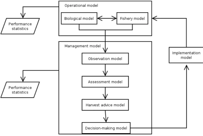
The way data are collected from the fishery is replicated by the observation model (ICES 2004). This includes not only fishery data but all data sources that might be used in either stock assessment or the definition of Harvest Control Rules (HCR) (McAllister et al. 1999). The conceptual framework followed here (see Figure 2) incorporates it as part of the management procedure, and not strictly within the operational model. Uncertainty in the collection of both fishery-dependent and independent data can be simulated by assigning probability distributions that reflect the error, know or assumed, around each step of the sampling procedure. Monte Carlo procedures are then implemented that, randomly sampling from those distributions, generate alternative states

of nature regarding those parameters, which can then be input to the next step in the procedure, the assessment model.

A number of possible sources of uncertainty are being incorporated in the bigeye tuna base case scenario. These were identified as the most likely relevant. Relatively simple formulations are being used at this stage, to easily understand the relative influence of each factor in the final uncertainty. In contrast with this approach, the data collection procedure could also be replicated by a series of sub-models that attempt to mimic the different stages involved (recording of landings, estimation of discards...). Such extra level of complexity would only be justified if the initial simulation procedure shows data collection and transformation to be an important component in the final uncertainty, or if the qualities of alternative sampling strategies needed to be evaluated.

Natural mortality and weight matrix

Uncertainty in the estimates of natural mortality, M, and the weight-at-age matrix, SWT, can have a significant impact on estimated values for spawning stock biomass, SSB, recruitment, R, and yield-per-recruit, Y/R. Our base case summarises the uncertainties around both M and SWT generating M and SWT matrix that include a lognormal error for all ages and period, with alternative CVs of 0.1 and 0.2.

The set of n (i = 1,..., n) SWT and M matrices thus generated are then combined with the VPA-estimated matrix of numbers at age and the estimated maturity to arrive at a set of SSB estimates. When the uncertainty in one or other parameter is incorporated separately, their individual effect on the estimate of SSB can be assessed.

Catch-at-age

Estimation of catch-at-age is generally considered to introduce significant uncertainty in the assessment process (ICES, 2004b). Errors in catch-at-length, aging and slicing combine in most cases to provide to the stock assessment process with a catch-at-age matrix that includes significant uncertainty in both the absolute and relative values for each age.

Uncertainty in the catch-at-age matrix for bigeye will be considered to originate mainly through the parameters of the growth equation. Two alternative models have been proposed for Atlantic bigeye (Alves et al. 1998 and Cayre and Diouf 1984). Both will be considered as equally probable and the differences in stock size estimates and subsequent decisions derived from them will be evaluated.

Assessment and management model

After data have been “collected” from the simulated population and fishery, a process of stock assessment attempts to estimate stock size and population trends. We are thus proposing the evaluation of model-based HCRs (McAllister et al., 1999), where stock assessment takes place before a decision on management is made. Although a combination of data-based and model-based rules could be conceived, as assessments of tropical tuna stocks under ICCAT's responsibility do not take place every year.

The actual process presently in place in ICCAT, based on a combination of production and age-structured models, could be replicated. It is however envisaged that the base case scenario will consist of a single model assessment, based on cohort analysis (VPA-ADAPT).

Example of implementation

In this example we use the library FLR generated in R language as part of the FEMS integrated fisheries modelling and simulation framework to show the differences of the effects of the uncertainties in the natural mortality on the estimation of recruitment.

The FLR library includes different objects such as FLQuant, defined as an array of five dimensions: age, year, stock, season and area. Natural mortality, M, has this structure, and it is included into another superior structure, the FLStock object. For each stock, the corresponding FLStock has associated another FLQuant object called FLCPUEs that contains the series of CPUEs indexes used for tuning the VPA. In this example we are going to apply to the simulated data for assessment the Extended Survivors Analysis (XSA) included as object FLXSA of the library FLR. For this proposal we use the following procedure:

1. Incorporate uncertainty in the M matrix of the base case creating a matrix whose elements follow a lognormal distribution with a specific coefficient of variation, and multiplying both matrices to obtain a new matrix of stochastic values of m for age and year.

2. At this point we start running 100 simulations resampling the columns of the new M matrix with replacement.

3. For each simulated matrix of values of M, run an XSA, applying the FLXSA method.

The outputs of the FLXSA are the abundances, so from this point we can obtain the recruitment, as the first row of the matrix for age 0, or the spawning stock biomass, as the product of N*mat*swt.

We consider in this case the effect of incorporating uncertainty in M on the recruitment, assigning a coefficient of variation of 10% and 20% to the lognormal matrix generated at the beginning of this section. To implement some diagnostics that show the differences between these options, we define, for each year, the standardized residuals as the difference between the simulated recruitments and the recruitment of the base case divided all by the standard deviation of the simulated recruitments, e.g.,

simulation j year i cruitment Simulated case base cruitment cruitment Simulated Rst j j i j i j i = = − = , , ) Re . var( ) . . Re Re . ( , , , (23)

For each alternative of the values of the coefficient of variation of the lognormal distribution of the error in m, 10% and 20%, Figures 3 and 4 show, respectively, the simulated recruitment for each year, the standardized residuals by year, the normal qq.plot of the standardized residuals and the AR(1) plot of the standardized residuals. To compare graphically results of both simulations, we plot a histogram of each standardized residual in Figure 5. These plots show that the residuals are more symmetric and have approximately a normal distribution in the case of the lower coefficient of variation. Also we can confirm that uncertainty in the M parameter is important, measured by its coefficient of variation, as differences in this value produce significantly different values of recruitment.

To consider the effect of uncertainty in M on the spawning stock biomass, assigning a coefficient of variation of 10% and 20% to the lognormal matrix generated at the beginning of this section, we can produce the same graphics as in the case of the recruitment, and compare if the effect of the variability in M is different. Another example of analysis that could be implemented in this framework is the analysis of the effect of uncertainties in the medium weights of the stock matrix, swt, over the recruitment and the spawning stock biomass, as well as on the yield-per-recruit analysis, and compare which of the two uncertainties has a larger effect on those matrices.

Conclusions

We have shown an initial example of the possibilities for use of this simulation framework. For the tropical species case study currently under development, the operational model will be implemented for the three species in the fishery (bigeye, yellowfin and skipjack) and different hypothesis of management interest will be tested. Some of the possible hypotheses already put forward for testing are:

1 Is the management procedure robust to the uncertainty posed by the difficulty of separating species in juvenile tuna.

2 Are the management procedures designed to protect juvenile tuna robust to the level of uncertainty present in M?

3 Can current management procedures cope with a shift in selectivity towards small tunas?

Present uncertainties in the stock assessment and management procedures presently in place for tropical tuna, can be examined coherently with a procedure as the one outlined here, and provide for both guidelines for research needs and solid management rules. The open nature of the development process within the FEMS project would allow for greater transparency and independent scrutiny of the work of the scientific bodies integrated in all international tuna commissions.

References

ALVES, A., P. de Barros, M.R. Pinho. 1998. Age and growth of bigeye tuna Thunnus obesus captured in the Madeira archipielago. ICCAT Col. Vol. Sci. Pap. 48(2): 277-283.

CAYRE, P., T. Diouf. 1984. Growth of Atlantic bigeye tuna (Thunnus obesus) according to tagging results. ICCAT Coll. Vol. Sci. Pap., 20(1): 1890-187.

ICES. 2004. Report of the Working Group on Methods. Lisbon. Report of the Workshop on Statistical Analysis of Sampling Data. Nantes. Unpubl. report.

MCALLISTER, M., P.J. Starr, V. Restrepo, G.P. Kirkwood. 1999. Formulating quantitative methods to evaluate fishery-management systems: what fishery processes should be modelled and what trade-offs should be made? ICES J. Mar. Sci. 56: 900-916.

KELL, L.T., D. J. Die, V.R. Restrepo, J.-M. Fromentin, V. Ortiz de Zárate, P. Pallarés. 2003. An evaluation of management strategies for Atlantic tuna stocks. Sci. Mar. 67: 353-370.

PARKS, W., F. X. Bard, P. Cayre, S. Kume, A. Santos Guerra. 1982. Length-weight relations for bigeye tuna captured in the eastern Atlantic Ocean. ICCAT. Col. Vol. Sci. Pap. 17(1): 214-225.

PORCH, C.E. 2003. Peliminary assessment of Atlantic white marlin (Tetrapturus albidus) using a state-space implementation of an age-structured production model. ICCAT. Col. Vol. Sci. Pap. 55(3): 559-577. PUNT, A.E., D.S. Butterworth. 2003. Specifications and clarifications regarding the ADAPT VPA

assessment/projection computations carried out during the September 2000 ICCAT West Atlantic bluefin tuna stock assessment session. ICCAT. Col. Vol. Sci. Pap. 55(3): 1028-1040.

Table 1. The stocks harvested by the six fleets defined in the study (note X - species targeted, X* - intermediate

sizes targeted, x - harvested as a by-catch).

Case studies

Bigeye Yellowfin Skipjack

Fleets Adults Juveniles Adults Juveniles

1. US Longline X

2. Asiatic Longline X X

3. Venezuelan Purse Seine X* X* X

4. European Purse Seine x X X X

5. Ghanaian Mixed Fleet X X X

6. Tropical Bait Boats X X X* X* X

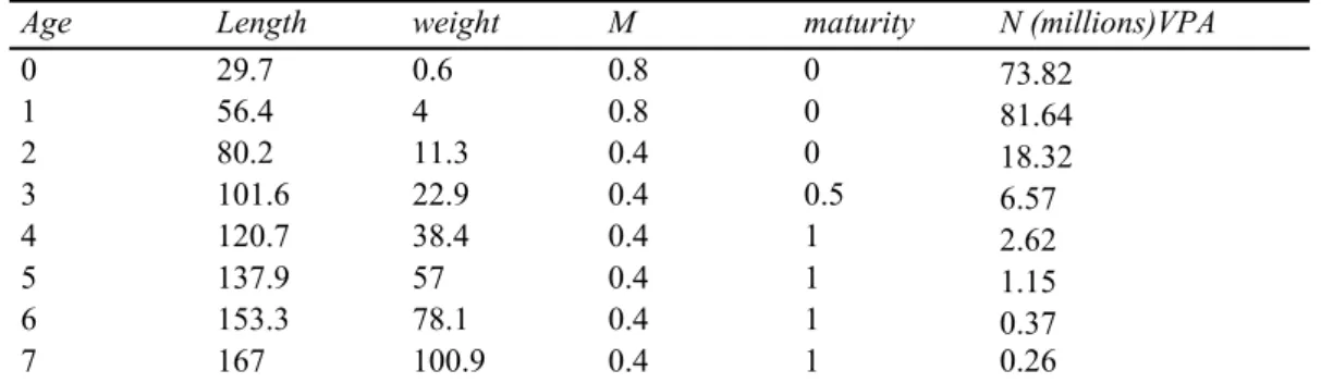
Table 2. Biological parameters and abundance estimates used in the base case.

Age Length weight M maturity N (millions)VPA

0 29.7 0.6 0.8 0 73.82 1 56.4 4 0.8 0 81.64 2 80.2 11.3 0.4 0 18.32 3 101.6 22.9 0.4 0.5 6.57 4 120.7 38.4 0.4 1 2.62 5 137.9 57 0.4 1 1.15 6 153.3 78.1 0.4 1 0.37 7 167 100.9 0.4 1 0.26

Table 3. Selectivity (1985-2001) by fleet obtained from a forward cohort analysis assuming constant

recruitment.

Age PS Ghanean PS-BB Tropical BB USA LL Asiatic LL Other

0 0.78 0.59 0.21 0.00 0.00 0.66 1 1.00 1.00 0.98 0.01 0.01 1.00 2 0.28 0.03 1.00 0.26 0.19 0.35 3 0.14 0.01 0.67 1.00 0.62 0.34 4 0.06 0.01 0.22 0.75 1.00 0.25 5 0.06 0.03 0.06 0.33 0.87 0.18 6 0.06 0.04 0.03 0.08 0.53 0.09 7+ 0.03 0.02 0.06 0.02 0.32 0.03

Selectivity pattern by fleet

0.00 0.20 0.40 0.60 0.80 1.00 1.20 0 1 2 3 4 5 6 7+ age P S G hanean P S-B B T ro pical B B USA LL A siatic LL O ther

1 9 7 5 1 9 8 0 1 9 8 5 1 9 9 0 1 9 9 5 2 0 0 0 3 e+ 07 5 e+ 07 7 e+ 07 y e a r R ec. v1 m l o g n o r m a l C V = 1 0 % . R e c r u it s b y Y e a r 1 9 7 5 1 9 8 0 1 9 8 5 1 9 9 0 1 9 9 5 2 0 0 0 -2 0 2 4 y e a r st dR e s. v1 S t a n d a r i s e d R e s i d u a ls b y Y e a r - 3 - 2 - 1 0 1 2 3 -2 0 2 4 N o r m a l Q - Q P l o t T h e o r e t i c a l Q u a n t i l e s Sa m pl e Q ua n til es - 2 0 2 4 -2 0 2 4 s t d R e s . v1 [ 2 : 2 7 0 0 ] st dR es .v 1[ 1: 26 99 ] A R ( 1 ) p lo t o f t h e r e s id u a ls

Figure 3. Results of the lognormal distribution with CV=10% of the error in M. Figure 2. Simulation model structure.

1 9 7 5 1 9 8 0 1 9 8 5 1 9 9 0 1 9 9 5 2 0 0 0 2. 0 e + 07 6. 0 e+ 07 1. 0 e+ 08 y e a r Rec .v m l o g n o r m a l C V = 2 0 % . R e c r u i t s b y Y e a r 1 9 7 5 1 9 8 0 1 9 8 5 1 9 9 0 1 9 9 5 2 0 0 0 -2 02 46 y e a r st dR es .v S t a n d a r i s e d R e s i d u a l s b y Y e a r - 3 - 2 - 1 0 1 2 3 -2 0 2 4 6 N o r m a l Q - Q P l o t T h e o r e t i c a l Q u a n t i l e s S am ple Q ua nt ile s - 2 0 2 4 6 -2 0 2 4 6 s t d R e s . v [ 2 : 2 7 0 0 ] st dRes .v [1 :2 699 ] A R ( 1 ) p l o t o f t h e r e s i d u a l s H i s t o g r a m o f r e s id u o s 1 0 2 0 [ , 2 ] r e s i d u o s 1 0 2 0 [, 2 ] Fr eque nc y - 2 0 2 4 6 0 100 200 30 0 400 50 0 H is t o g r a m o f r e s i d u o s 1 0 2 0 [ , 1 ] r e s i d u o s 1 0 2 0 [, 1 ] Fr eque nc y - 2 0 2 4 6 0 100 20 0 3 00 40 0 5 00 60 0 700

Figure 4. Results of the lognormal distribution with CV=20% of the error in m.