Identity recognition based on the external shape of the human ear

Identity Recognition Based on the External Shape of

the Human Ear

Amir Benzaoui, Nabil Hezil, and Abdelhani Boukrouche

Department of Electronics and Telecommunications University of May 08th _{1945, B.P box 401, Guelma 24 000, Algeria}

benzaoui.amir@univ-guelma.dz hani.boukrouche@pimis.net Abstract—External shape of the human ear presents a rich

and stable information embedded on the curved 3D surface, which has invited lot attention from the forensic and engineer scientists in order to differentiate and recognize people. However, recognizing identity from external shape of the human ear in unconstrained environments, with insufficient and incomplete training data, dealing with strong person-specificity, and high within-range variance, can be very challenging. In this work, we implement a simple yet effective approach which uses and exploits recent local texture-based descriptors to achieve faster and more accurate results. Support Vector Machines (SVM) are used as a classifier. We experiment with two publicly available databases, which are IIT Delhi-1 and IIT Delhi-2, consisting of several ear benchmarks of different natures under varying conditions and imaging qualities. The experiments show excellent results beyond the state-of-the-art.

Keywords—Biometrics; Identity; Ear Recognition; Texture Analysis; BSIF.

I. INTRODUCTION

Biometric systems have an important role in the information and public security domains. They provide an automatic identification or verification of the identity based on the analysis of physical, chemical, or behavioral modalities of the human body. Several modalities have been proposed to recognize the human identity, we can cite: face, fingerprint, iris, palmprint, signature, or gait [1-3].

The use of the human ear in forensic and biometric applications has become a quite interesting way in the last few years. It is considered as a new class of biometrics which is not yet used in real context or in commercial applications. The external shape of the human ear is characterized by a rich structure which provides sufficient and important information to differentiate and recognize people; we can visualize 10 features and 37 sub-features from 2D ear imaging. The terminology of the human ear is presented in Fig.1; this terminology is made up of standard features. It includes an outer rim (Helix) and ridges (Antihelix) parallel to the helix,

the concha (hollow part of the ear), the lobe and the tragus (small prominence of cartilage) [4-6]. The human ear has several advantages compared to other modalities: it has a rich structure, smaller object (small resolution), stable over time, modality accepted by people, the acquisition of the ear imaging can be affected without participation of the subject and can be captured from distance, and not affected by changes in age, facial expression, position, and rotation.

Fig. 1. Terminology of the human ear [5].

An ear recognition system can be divided into three main steps: ear normalization, feature extraction and classification. In the normalization step, the ear image must be normalized to standard size and direction according to the long axis of outer ear contour (see Fig.2). The long axis was defined as the line crossing through the two points which have the longest distance on the ear contour [7]. After normalization, the long axes of different ear images were normalized to the same length and same direction. The next steps are to represent the ear by appropriate features and design effective classifier. Most researches on ear biometrics are focused on feature extraction and classification. In real applications, however, the big challenge of ear recognition is how to find an efficient descriptor to represent and to model the human ear in a real context where the ear can be affected by illumination variation, pose variation, noise, or occlusion.

(a) (b) (c) (d) Fig. 2. Example of ear normalisation to standard size and direction [7]. (a)

long axis detection, (b) rotation, (a) cropping, and (d) resize.

The paper is structured as follows: next section gathers and comments some previous related work of ear biometric recognition. The candidate descriptors to be evaluated are reviewed in Section 3, along with the selected pre-processing and classification schemes. Evaluation is presented out in Section 4, by first describing available databases, and subsequently analyzing the extensive experiments carried out over the investigations of local texture descriptors. Finally, Section 5 summarizes the results and draws some conclusions.

II. RELATED WORK

The idea of the French criminologist Alphonse Bertillon in 1890 was considered as the first jump if the field of recognizing people by using their ear’s shape [8]. After that, Iannareli et al. [9] have developed the first system of ear classification based on manual measurements in 1949. This system has been used for more than 40 years in the United States; it has played an important role in forensics and criminal investigations. The first computerized system based on ear modality was developed in 1997 by Burge and Burger [10,11]; this system was based on graph matching techniques with Vornoi diagram of curves extracted from the contours. PCA or Eigen-Ear was also implemented to extract features and recognize persons by using their ears [12]; PCA seeks for a suitable space of low-dimensional representation, constructed from a set of training images, which preserves the properties of the original data as much as possible [13]. The Force Field Transform was proposed by Hurley et al. [14,15] and also applied to ear recognition; the ear image is considered as an array of mutually attracting particles that act as the source of a Gaussian force field. After ear’s transformation, the force field was converted to convergence field, and the Fourier based cross-correlation is applied to perform multiplicative template matching that exceed a fixed threshold. The experimental results of this approach have showed good performances compared to PCA in unconstrained cases. Basit et al. [16] have used nonlinear Curvelet Transform and k-NN classifier for identification. The features of the ear are extracted by rapplying the Fast Discrete Curvelet Transform (FDCT) via the wapping technique. The

feature vector of each image is composed of approximate curvelet coefficients at eight different angles. Recently, the 3D model of the ear was also explored [5,17-19]. The 3D models usually achieve high accuracy rates compared to 2D imaging. While the 3D models have the advantage of suffering less from pose, lighting, or noise, they are also less suitable in real-world applications as they require expensive and complex computation with specific equipments.

Unlike previous works, we propose in this paper the use of local texture descriptors for automated human identification using 2D ear imaging in unconstrained conditions. We particularly consider three recent yet very popular descriptors namely Local Binary Patterns (LBP) [20], Local Phase Quantization (LPQ) [21] and Binarized Statistical Image Features (BSIF) [22]. BSIF is inspired by LBP and LPQ methodologies. These descriptors describe each pixel’s neighborhood by a binary code which is obtained by first convolving the image with a set of linear filters and then binarizing the filter responses. The bits in the code string correspond to binarized responses of different filters. However, in contrast to earlier approaches, such as LBP and LPQ, BSIF does not use a manually predefined set of filters but learn the filters from statistics of natural images using Independent Component Analysis (ICA) [23].

III. METHODOLOGY

The proposed biometric system requires two operational phases. The first is a training phase: it consists in recording the ear features of each individual in order to create his own biometric template; this is then stored in the database. The second is the test phase: it consists in recording the same features and comparing them to the biometric templates stored in the database. If the recorded data match a biometric template from the database, the individual in such a case is considered identified.

The proposed biometric system based on external shape of 2D ear imaging is described in the following modules:

A. Pre-processing

The objective of the pre-processing module is to prepare the source image representation in order to facilitate the task of the following steps and to improve the recognition performances. First, the ear imaging is converted into gray-scale image. Next, every gray-gray-scale image is filtered by median filter to reduce noise. This filtered image is then adjusted to improve the image contrast [24].

B. Feature Extraction

The choice of visual features to be extracted from normalized ear images and sent for classification plays an

important role on the resulting recognition accuracy. paper, we have selected a number of recent

descriptors that are distinctive, do not require segmentation, and robust to occlusion, illumination variation, and weak lighting. In contrast to global image descriptors which compute features directly from the entire image, local descriptors representing the features in small local image patches have proven to be more effective in real conditions. We present below the three implemented local texture descriptors, namely LBP, LPQ, and BSIF.

The Local Binary Patterns (LBP) [ analysis operator, introduced by Ojala et al.

a gray-scale invariant texture measure, and derived

general definition of texture in a local neighborhood. It is a powerful mean of texture description and among its pro in real-world applications are its discriminative power, computational simplicity and tolerance against monotonic gray-scale changes. In the original LBP operator, the local patterns are extracted by thresholding the 3×3 neighborhood of the eight neighbors of each pixel, from the original image, with the central value. All the neighbors are assigned

1 if they are greater than or equal to the current element and 0 otherwise, which represents a binary code of the central element. This binary code is converted into a

multiplying it with the given corresponding weights and summed to obtain the LBP code for the central value histogram of these 2 256 different labels can then be used as a texture descriptor for further analysis. Recently, the LBP operator has been extended to use neighborhoods of different sizes in order to capture the large-scale structures which can be considered as the dominant patterns in the image (for more details, see [24,26]).

The Local Phase Quantization (LPQ) [

in order to tackle the relative sensitivity of LBP to blur, based on quantizing the Fourier transform phase in local neighborhoods. The phase can be shown to be a blur invariant property under certain commonly fulfille

texture analysis, histograms of LPQ labels computed within local regions are used as a texture descriptor similarly to the LBP methodology. The LPQ descriptor has recently received wide interest in blur-invariant texture recognition. LPQ i insensitive to image blurring, and it is has proven to be very efficient descriptor in pattern recognition from blurred as well as from sharp images.

The Binarized Statistical Images Features (BSIF) was recently proposed for texture classification.

LBP and LPQ, the idea behind BSIF is to automatically learn a fixed set of filters from a small set of natural images, instead of using hand-crafted filters such as LBP and LPQ. important role on the resulting recognition accuracy. In this

recent local texture distinctive, do not require segmentation, and robust to occlusion, illumination variation, and weak In contrast to global image descriptors which compute features directly from the entire image, local res in small local image patches have proven to be more effective in real-world We present below the three implemented local texture descriptors, namely LBP, LPQ, and BSIF.

[20] is a texture [25], is defined as and derived from a general definition of texture in a local neighborhood. It is a powerful mean of texture description and among its properties world applications are its discriminative power, computational simplicity and tolerance against monotonic In the original LBP operator, the local patterns are extracted by thresholding the 3×3 neighborhood eighbors of each pixel, from the original image, are assigned the value or equal to the current element and 0 a binary code of the central code is converted into a decimal value by with the given corresponding weights and is summed to obtain the LBP code for the central value. The different labels can then be used nalysis. Recently, the LBP operator has been extended to use neighborhoods of different scale structures which can in the image (for more [21] was proposed in order to tackle the relative sensitivity of LBP to blur, based on quantizing the Fourier transform phase in local The phase can be shown to be a blur invariant property under certain commonly fulfilled conditions. In texture analysis, histograms of LPQ labels computed within local regions are used as a texture descriptor similarly to the The LPQ descriptor has recently received invariant texture recognition. LPQ is insensitive to image blurring, and it is has proven to be very efficient descriptor in pattern recognition from blurred as well The Binarized Statistical Images Features (BSIF) [22] classification. Inspired by LBP and LPQ, the idea behind BSIF is to automatically learn a fixed set of filters from a small set of natural images, instead crafted filters such as LBP and LPQ. BSIF

applies learning, instead of manual tuning, t

statistically meaningful representation of the images, which enables efficient information encoding using simple element wise quantization. Learning provides also an easy and flexible way to adjust the descriptor length and to adapt applications with unusual image characteristics.

properties within each image sub

pixels’ BSIF code values are then used. The value of each element (i.e. bit) in the BSIF binary code string is computed by binarizing the response of a linear filter with a threshold at zero. Each bit is associated with a different filter and the desired length of the bit string determines the number of filters used. The set of filters is learnt from a training set of natural image patches by maximizing the statistical independence of the filter responses.

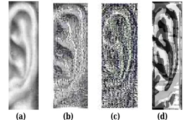
Fig.3 shows an example of normalized ear image and their corresponding LBP (8,1), LPQ

representations, respectively.

(a) (b)

Fig. 3. (a) Example of normalized ear images and their

LBP (8,1), (c) LPQ3, and (d) BSIF (with C. Classification

Regarding the learning algorithm, several approaches have been proposed, including, among others, neural

their invariant, Support Vector Machines (SVM) / Support Vector Regressors (SVR), Random Forests (RF), and projection techniques such as C

(CCA)… From the wide variety of learning schemes presented in the literature, Support Vector Machines (SVM) and its derivations have recently obtained state

challenging large databases [27] IV. EXPERIMENTA

A. Dataset

The IIT Delhi database

collected from students and staff at IIT (India). It was acquired on the IIT Delhi 2006 to June 2007 using a simple imaging images were acquired from a distance in

applies learning, instead of manual tuning, to obtain statistically meaningful representation of the images, which enables efficient information encoding using simple element-wise quantization. Learning provides also an easy and flexible way to adjust the descriptor length and to adapt applications ith unusual image characteristics. To characterize the texture properties within each image sub-region, the histograms of pixels’ BSIF code values are then used. The value of each element (i.e. bit) in the BSIF binary code string is computed the response of a linear filter with a threshold at zero. Each bit is associated with a different filter and the desired length of the bit string determines the number of filters used. The set of filters is learnt from a training set of natural es by maximizing the statistical independence of Fig.3 shows an example of normalized ear image and their corresponding LBP (8,1), LPQ3, and BSIF (with 9, 8)

(c) (d)

Example of normalized ear images and their corresponding (b)

BSIF (with 9 and 8) representations.

Regarding the learning algorithm, several approaches have been proposed, including, among others, neural networks and their invariant, Support Vector Machines (SVM) / Support Vector Regressors (SVR), Random Forests (RF), and projection techniques such as Canonical Correlation Analysis From the wide variety of learning schemes presented in the literature, Support Vector Machines (SVM) and its derivations have recently obtained state-of-the-art results in

[27].

XPERIMENTAL RESULTS

The IIT Delhi database [28] consists of ear images collected from students and staff at IIT Delhi, New Delhi . It was acquired on the IIT Delhi campus from October 2006 to June 2007 using a simple imaging setup. All the acquired from a distance in an indoor

environment. The currently available database has two versions: the first version contains 493 images of 125 different subjects (IIT Delhi-1) and the second version contains 793 images of 221 different subjects (IIT Delhi-2). Each subject in the database has at least three ear images. The subjects are in the age range of 14 to 58 years. The resolution of the images is 272 × 204 pixels. In addition to the original images, this database also comes with automatically normalized and cropped ear images of 50 × 180 pixels in size.

B. Settings

In the first protocol (“experiments using two images per person as training set”), two ear images from each person in the database were used as the “training set” and the remaining ear images of the same person (i.e., from one to four images) were used as the “test set.” Since most of the samples in the two databases have three images, we conducted three permutations and report the average rates (This is the most widely used protocol in literature). In the second protocol (“experiments using single image per person as training set”), only one image from each person was used as the “training set”

and the remaining images of the same person (from two to five images) were used as the “test set.” We also did three permutations and report the average rates.

C. Experiments

In our experiments, we tested the several parameters of the local texture descriptor i.e., the LBP was tested under several scale sizes (P,R), the LPQ descriptor was implemented with different radius, and the BSIF descriptor was implemented with several filter parameters (filter size and bit string: and ). Two types of SVM classifier were compared and used for classification: SVM with linear kernel and SVM with RBF kernel, we selected the two most widely used kernel functions, i.e., linear and RBF. The parameter in the RBF kernel function was empirically selected in this paper (γ = 0.0001). Table 1 compares the rank-1 recognition results using two images in the training set and the two classifiers cited above applied to the IIT Delhi-1 and IIT Delhi-2 databases. Table 2 compares the rank-1 recognition results using single image per person in the training set and the two classifiers applied to the two databases.

The best results of the LPQ descriptor were given with a radius = 3 and the best results of the BSIF descriptor were obtained with a window size of 15×15 pixels and 12 bits. As can be seen from Tables 1 and 2, the best recognition performances on both datasets are obtained with the Linear Kernel of the SVM classifier. The LBP descriptor seems to work better with large scale sizes than with smaller scale sizes. The results obtained indicate that LPQ outperforms LBP under

different settings and BSIF gives the best performances. In addition, surprising and very interesting results appeared with the BSIF descriptor using only single image as a reference in the training set (> 90%).

TABLE I. BEST OF RANK-1 RECOGNITION RATES IN THE 1ST _SCENARIO Descriptor IIT Delhi-1 IIT Delhi-2

Linear kernel RBF kernel Linear kernel RBF kernel

LBP (8,1) 77.50 73.94 74.74 71.51 LBP (8,2) 80.38 67.82 79.2 67.88 LBP (8,3) 81.62 62.55 80.53 64.96 LBP (16,2) 71.68 66.26 78.16 68.00 LPQ 79.84 79.79 79.77 79.87 BSIF 96.68 96.68 97.31 97.31

TABLE II. BEST OF RANK-1 RECOGNITION RATES IN THE 2ND _SCENARIO Descriptor IIT Delhi-1 IIT Delhi-2

Linear kernel RBF kernel Linear kernel RBF kernel

LBP (8,1) 63.32 63.32 57.28 57.23 LBP (8,2) 67.12 67.12 62.94 62.94 LBP (8,3) 68.21 68.21 64.63 64.63 LBP (16,2) 67.03 67.03 63.40 63.46 LPQ 73.82 73.82 71.5 71.5 BSIF 91.26 91.26 90.29 90.29 D. Comparison

For a comprehensive analysis, we also compared the results obtained against those of state-of-the-art automatic ear recognition. Table 3 shows and compares the average rank-1 recognition rate of the proposed method with some well known and recent feature extraction approaches under the same conditions and protocol of evaluation (the most widely used protocol in literature is “two images per person as training set”), to ear recognition using 2-D imaging. As can be seen, our proposed approach based on the BSIF descriptor shows a very competitive performance, outperforming other approaches under the same conditions.

TABLE III. RANK-1 COMPARISON TO SOME RECENT WORKS

Method Delhi-1 Delhi-2

Force Field Trnasform [15] 74.93 66.67

Orthogonal log-Gabor filter pair [29] 96.27 95.93

2D quadratures filter [30] 96.53 96.08

Local principal independent components [31] 97.60 97.20 Non Linear Curvelet Transform [16] 97.77 96.22

V. CONCLUSION

In our investigation, we have successfully implemented a feature extraction approach for automated 2D ear description and recognition. We have introduced the use of the local texture descriptors, which are inspired from the statistics of natural images and produce binary codes. In contrast to global approaches which compute features directly from the entire image, local descriptors representing the features in small local image patches have proven to be more effective in real-world conditions. A series of experimental evaluations on IIT Delhi-1 and IIT Delhi-2 databases show that this implemented approach of feature extraction, based on BSIF descriptor, given very significant improvements at the recognition rates, superiority in comparison to the state of the art, and a good effectiveness in the unconstrained cases.

References

[1] J.A. Unar, W.C. Seng, and A. Abbasi, “A Review of biometric technology along with trends and prospects,” Pattern Recognition (Elsevier), vol.47, no.8, pp.2673-2688, 2014.

[2] J. Ashbourn, editor “Biometrics in the new world: The cloud, Mobile technology, and Pervasive identity,” Springer Publishing Company, 2014.

[3] A.K. Jain, A.A. Ross, and K. Nandakumar, editors “Introduction to Biometrics,” Springer Science + Business Media, 2011.

[4] A.D. Dinkar and S.S. Sambyal, “Person identification in ethnic Indian goans using ear biometrics and neural networks,” Forensic Science International (Elsevier), vol.223, no.1-3, pp.373.e1-13, 2012.

[5] H. Chen and B. Bhanu, “Human ear recognition in 3D,” IEEE Transaction on Pattern Analysis and Machine Intelligence (PAMI), vol.29, no4, pp.718-737, 2007.

[6] A. Pflug and C. Busch, “Ear biometrics: a survey of detection, feature extraction and recognition methods,” IET Biometrics, vol.1, no.2, pp.114-129, 2012.

[7] L. Yuan and Z. Mu, “Ear recognition based on Gabor features and KFDA,” The Scientific World Journal (Hindawi), ID.702076, 2014. [8] A. Bertillon, “La photographie judiciaire, avec une apprendice sur la

classification anthropométriques,” Technical Report, Gauthier-Villars, Paris (France), 1980.

[9] A. Iannarelli, “Ear identification,” Forensic Identification Series, Technical Report, Paramount Publishing Company, Fremont, California (USA), 1989.

[10] M. Burge and W. Burger, “Ear biometrics in machine vision,” In Proceedings of the 21st _{Workshop of the Australian Association for}

Pattern Recognition, 1997.

[11] M. Burge and W. Burger, “Ear biometrics,” In A.K. Jain, R. Bolle, and S. Pankanti, editors “Biometrics: Personal Indentification in Networked Society,” Springer-Verlag, pp.273-286, 1998.

[12] K. Chang, K.W. Bowyer, S. Sarkar, and B. Victor, “Comparison and combinations of ear and face images in appearance-based biometrics,” IEEE Transactions on Pattern Analysis and Machine Intelligence (PAMI), vol.25, no9, pp.1160-1165, 2003.

[13] M. Turk and A. Pentland, “Eigenfaces for recognition,” Journal of Cognitive Neuroscience, vol.3, no.1, pp.71-86, 1991.

[14] D. Hurley, M. Nixon, and J. Carter, “Force field energy functional for image feature extraction,” Image Vision and Computing Journal (Elsevier), vol.20, no.5-6, pp.429-432, 2002.

[15] D. Hurley, M. Nixon, and J. Carter, “Force field energy functional for ear biometrics,” Computer Vision and Image Understanding (Elsevier), vol.98, no.3, pp.491-512, 2005.

[16] A. Basit and M. Shoaib, “A human ear recognition method using nonlinear curvelet feature subspace,” International Journal of Computer Mathematics (Taylor & Francis), vol.91, no.3, pp.616-624, 2014. [17] S. Cadivid and M. Abdel-Mottaleb, “3-D ear modeling and recognition

from video using shape from shading,” IEEE Transactions on Information Forensics and Security, vol.3, no.4, pp.709-718, 2008. [18] P. Prakash and P. Gupta, “A rotation and scale invariant technique for

ear detection in 3D,” Pattern Recognition Letters (Elsevier), vol.33, no.14, pp.1924-1931, 2012.

[19] J. Zhou, S. Cadivid, and M. Abdel-Mottaleb, “An efficient 3-D ear recognition system employing local and holistic features,” IEEE transactions on Information Forensics and Security, vol.7, no.3, pp.879-991, 2012.

[20] T. Ahonen, A. Hadid, and M. Pietikainen, “Face description with local binary patterns: application to face recognition,” IEEE Transactions on Pattern Analysis and Machine Intelligence (PAMI), vol.28, no.12, pp.2037-2041, 2006.

[21] V. Ojansivu and J. Heikkil, “Blur insensitive texture classification using local phase quantization,” In Proceedings of the 3rd _Internationl

Conference on Image and Signal Processing (ICSIP), Springer-Verlg, pp.236-243, 2008.

[22] J. Kannala and E. Rahtu, “BSIF: binarized statistical image features,” In Proceedings of the International Conference on Pattern Recognition (ICPR), pp.1363-1366, 2012.

[23] A. Hyvarinen and E. Oja, “Independent component anlysis: algorithms and applications,” Neurl Networks, vol.13, no.4-5, pp.411-430, 2000. [24] A. Benzaoui and A. Boukrouche, “1DLBP and PCA for face

recognition,” In Proceedings of the 11th _{IEEE International Symposium}

on Programming and Systems (ISPS), pp.7-11, 2013.

[25] T. Ojala, M. Pietikainen, and T. Maenpa, “Multiresolution gray-scale and rotation invariant texture classification with local binary patterns,” IEEE Transactions on Pattern Analysis and Machine Intelligence (PAMI), vol.24, no.7, pp.971-987; 2002.

[26] A. Benzaoui and A. Boukrouche, “Face analysis, description, and recognition using improved local binary patterns in one dimensional space” Journal of Control Engineering and Applied Informatics (CEAI), vol.15, no.1, pp.52-60, 2014.

[27] K.L. Du and M.N.S. Swamy, “Support Vector Machines,” In K.L. Du and M.N.S. Swamy, editors “Neural Networks and Statistical Learning,” Springer-Verlag, pp.469-524, 2014.

[28] A.Kumar, “IIT Delhi ear database version 1.0,” New Delhi, India, 2007: http://www4.comp.polyu.edu.hk/~csajaykr/IITD/Database_Ear.htm. [29] A. Kumar and C. Wu, “Automated human identification using ear

imaging,” Pattern Recognition (Elsevier), vol.45, no.3, pp.956-968, 2012.

[30] T.S. Chan and A. Kumar, “Reliable ear identification using 2-D quadrature filters,” Pattern Recognition Letters (Elsevier), vol.33, no.14, pp.1870-1881, 2012.

[31] Mamta and H. Madasu, “Robust ear based authentication using local principal independent components,” Expert Systems and Applications (Elsevier), vol.40, no.16, pp.6478-6490, 2013.