Asymptotic observers and integer programming for functional classification of a microbial community in a chemostat

HAL Id: hal-02734813

https://hal.inrae.fr/hal-02734813

Submitted on 1 Apr 2021

HAL is a multi-disciplinary open access

archive for the deposit and dissemination of

sci-entific research documents, whether they are

pub-lished or not. The documents may come from

teaching and research institutions in France or

abroad, or from public or private research centers.

L’archive ouverte pluridisciplinaire HAL, est

destinée au dépôt et à la diffusion de documents

scientifiques de niveau recherche, publiés ou non,

émanant des établissements d’enseignement et de

recherche français ou étrangers, des laboratoires

publics ou privés.

Asymptotic observers and integer programming for

functional classification of a microbial community in a

chemostat

Pablo Ugalde Salas, Jérôme Harmand, Elie Desmond-Le Quéméner

To cite this version:

Pablo Ugalde Salas, Jérôme Harmand, Elie Desmond-Le Quéméner. Asymptotic observers and integer

programming for functional classification of a microbial community in a chemostat. ECC19 - 18.

European Control Conference, European Control Association (EUCA). International Federation of

Automatic Control (IFAC)., Jun 2019, Naples, Italy. pp.1665-1670, �10.23919/ECC.2019.8795854�.

�hal-02734813�

Asymptotic Observers and Integer Programming for Functional

Classification of a Microbial Community in a Chemostat.

Pablo Ugalde-Salas

1

, J´erˆome Harmand

2

and Elie Desmond-Le Qu´em´ener

3

Abstract— From genetic sequencing, dry biomass, and metabolites measurements, the assignment of functions to the species present in chemostat experiments was solved by merging chemostat modelling and quadratic mixed integer program-ming. The method was tested on a nitrification bioprocess where two functions are known to drive the system. Sensitivity of the method, its advantages, and limitations are discussed.

I. INTRODUCTION

The objective of this manuscript is to present an opti-mization method based on mixed integer programming and invariants of chemostat dynamical models for the functional classification of microorganisms in bioprocess. One of the first attempts to implement an optimization procedure can be found in Dumont et al. [1].

Measurements based on genetic material have become standard practice in ecological engineered systems (e.g. wastewater treatments plants) [2]. However using this mea-surements for prediction and control is still at a very early stage. To face such challenges linking functionality to the different members of the community is an important initial task to be tackled [3], [4]. Comparisons of such measure-ments to current databases often fall short, since the coverage of existing species is very limited compared to reality. The motivation is therefore to develop tools for incorporating these new measurements in engineering models.

II. MATERIALS ANDMETHODS

Variables used throughout the article are summarized in Table I. The following conventions are used: Let n ∈ N then [n] := {1, . . . , n}, R+:= {t ≥ 0|t ∈ R}.

A. Experimental Conditions

The optimization method is applied to data coming from a chemostat experiment. A chemostat is an experimental device used to study microbial growth where a reactor continuously receives a solution containing nutrients for proper microbial development [5]. The reactor has the same inlet and outlet flow, thus a constant volume is maintained inside the reactor.

Two reactors, A and B, were operated continuously for approximately 500 days with variable dilution rate and substrate input. They were inoculated with wastewater sludge and a dilution composed of ammonium and a synthetic

1_{LBE, Univ Montpellier, INRA, 102 avenue des Etangs, 11100,}

Nar-bonne, France. Ph.D Student.pablo.ugalde-salas@inra.fr

2 _{LBE, INRA, Univ Montpellier, 11100, Narbonne, France.}

jerome.harmand@inra.fr

3 _{LBE, INRA, Univ Montpellier, 11100, Narbonne, France.}

elie.lequemener@inra.fr

mineral medium was used; as a consequence a nitrification process took place. Oxygen injection was maximized so there was no oxygen limitation, and pH was regulated and maintained around 7.

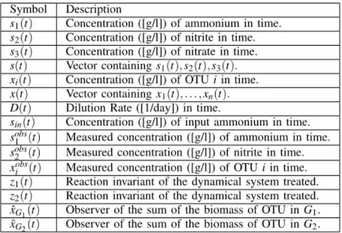
TABLE I: Notation used throughout the article.

Symbol Description

s1(t) Concentration ([g/l]) of ammonium in time.

s2(t) Concentration ([g/l]) of nitrite in time.

s3(t) Concentration ([g/l]) of nitrate in time.

s(t) Vector containing s1(t), s2(t), s3(t).

xi(t) Concentration ([g/l]) of OTU i in time.

x(t) Vector containing x1(t), . . . , xn(t).

D(t) Dilution Rate ([1/day]) in time.

sin(t) Concentration ([g/l]) of input ammonium in time.

sobs

1 (t) Measured concentration ([g/l]) of ammonium in time.

sobs₂ (t) Measured concentration ([g/l]) of nitrite in time. xobs_i (t) Measured concentration ([g/l]) of OTU i in time. z1(t) Reaction invariant of the dynamical system treated.

z2(t) Reaction invariant of the dynamical system treated.

ˆ

xG1(t) Observer of the sum of the biomass of OTU in G1.

ˆ

xG2(t) Observer of the sum of the biomass of OTU in G2.

Samples of the total dry biomass, concentrations of ammo-nium (NH4+), nitrite (NO2–), and nitrate (NO3–), were taken

at specific times. Microbial diversity was analyzed using single strand conformation polymorphism (SSCP) at specific times: 44 different Operational Taxonomic Unit (OTU) were identified in total, with most of them being present in both. More details on the experimental conditions can be found in the author’s original article [6].

B. Stoichiometry and Functional Groups

For this article a cascade (bio)reaction process is consid-ered. Suppose n different OTU are present in the chemo-stat. The cascade reaction refers to the situation where a

group of microorganisms (G1⊂ [n]) consumes a substrate

s1 and produces s2 and biomass, while another group of

microorganisms (G2⊂ [n]) consumes s2 and produces s3

and biomass. G1 and G2 are called functional groups. The

situation is described as simplified reactions (R1) and (R2). The reactions are simplified in the sense that they do not attempt to represent a balanced chemical reaction, rather it represents the direction of the bioprocess and the propor-tions (stoichiometric coefficients) of different consumed and formed compounds of interest.

s1 µi(s,x) −→ s2+ yiMx ∀i ∈ G1 (R1) s2 µi(s,x) −→ s3+ yiMx ∀i ∈ G2 (R2)

The terms yi are known as yields, it represents the

num-ber of moles of biomass produced per mole of substrate consumed. However in this work the unit grams of dry biomass per gram of substrate is used for yields. The term

Mxrepresents a molecule of biomass and several expressions

can be found in the literature (e.g. CH1.613O0.557N0.158 [7]).

Furthermore, for each i ∈ [n], OTU i is characterized by its process rate (also known as growth function or kinetics) µi(s, x), where the first variable s represents a vector

con-taining the concentration of (s1, s2, s3). The second variable

x represents the vector containing the concentration of all

OTU.

From an evolutionary perspective there is reason to think that each OTU may have its own yield and growth function. From biological knowledge it is sometimes known that two different OTU can not belong to the same functional group, that is G1∩ G2= /0. This is the case of nitrification

process [8]. The group G1 is known as ammonia oxidizer

Bacteria (AOB), which turn ammonia (s1) into nitrite (s2),

the group G2 is known as nitrite oxidizer Bacteria (NOB)

which turns nitrite into nitrate (s3).

C. Mass-Balanced model

The cascade reaction is modelled as a substrate-coupled dynamical model.

The chemostat has a dilution rate of D and an input of

ammonium concentration sin, both of which are operating

parameters that can change in time, that is D = D(t) and sin=

sin(t), however for alleviating notation the time dependence

is dropped. For more details in chemostat modelling the reader may refer to [9].

Denoting each OTU concentration by xi, ammonium by

s1, nitrite by s2, nitrate by s3, and considering reactions

(R1), and (R2) the mass balanced model can be formally expressed: ˙ xi= (µi(s, x) − D) xi ∀i ∈ G1 (1) ˙ xi= (µi(s, x) − D) xi ∀i ∈ G2 (2) ˙ s1=(sin− s1)D −

∑

i∈G₁ 1 yi µi(s, x)xi (3) ˙ s2= − s2D+

_∑

i∈G1 1 yi µi(s, x)xi−

∑

i∈G2 1 yi µi(s, x)xi (4) ˙ s3= − s3D+

_∑

i∈G1 1 yi µi(s, x)xi (5)

At this point we can formally state the problem. Let us assume that we know the measurements of the abundance

of n OTU xobs

i (t) i ∈ [n], sobs1 (t), sobs2 (t), and sobs3 (t) in a

chemostat where sin and D(t) are known. Find two disjoint

subsets G1, G2⊂ [n], such that the norm of the difference of

the observations and the solution of the system (x, s) given

by equations (1), (2), (3), (4), and (5) is minimized, that is

min ∑ i∈G1 kxi− xobsi k2+ ∑ i∈G2 kxi− xobsi k2 +ks₁− sobs 1 k2+ ks2− sobs2 k2+ ks3− sobs3 k2 s.t G1, G2⊂ [n] G1∩ G2= /0 (x, s) solution of (1), (2), (3), (4), (5) (6)

The problem lies on (i) not knowing the growth rates and (ii) testing all the possible combinations and simulating is computationally expensive.

D. Asymptotic Observer

If we knew a priori both sets G1and G2 and the growth

rates µi(x, s), then we could directly compare the

measure-ments and the dynamical system given by equations (1), (2), (3), (4), and (5). However we do not know neither the sets nor the kinetics.

To solve this problem a classic invariant of such types of model are derived. These are called also reaction invariants [10]. They allow the construction of asymptotic observers [11], which are observers in the sense that, whatever the initial conditions are, they converge to a manifold which only depends on the yields and some state variables, thus circumventing the knowledge of process rate; this has been done for general biochemical reactors (equations (49) to (56)) in [11]. The price to pay for such observers is that the convergence rate to the manifold depends on the operating conditions.

Define z1:= ∑

i∈G₁ 1

yixi+ s1and compute ˙z1using equations

(1) and (3): ˙ z1=

_∑

i∈G1 1 yi ˙ xi+ ˙s1 (7) =

_∑

i∈G₁ 1 yi (µi(s, x) − D) xi+ (sin− s1)D −

∑

i∈G₁ 1 yi µi(s, x)xi (8) = −D

_∑

i∈G1 1 yi xi+ s1− sin ! (9) = −D(t)(z1− sin(t)) (10)

Analogously another invariant can be derived that allows

linking the biomass of G2 and substrates. Define z2:=

∑

i∈G₂ 1

yixi+ s1+ s2 and compute ˙z2 using equations (2), (3),

˙ z2=

∑

i∈G2 1 yi ˙ xi+ ˙s1+ ˙s2 (11) =

_∑

i∈G2 1 yi (µi(s2, x) − D) xi+ (sin− s1)D (12) −

_∑

i∈G₁ 1 yi µi(s1, x)xi− s2D+

_∑

i∈G₁ 1 yi µi(s1, x)xi −

_∑

i∈G₂ 1 yi µi(s2, x)xi (13) = −D

_∑

i∈G2 1 yi xi+ s1+ s2− sin ! (14) = −D(t)(z2− sin(t)) (15)

Note that z1and z2satisfy the same dynamics, which does

not depend in µi. Invariants z1 and z2 can be shown to be

stable [11].

A simulation of the differential equation (10) using the dilution rate and input ammonium of the experiment can be seen in Fig. 1, it suggests that the solutions approach rapidly to a similar curve independently of the initial point. Since at the beginning of the experiment minimal biomass

is present one assumes z1(0) =

∑

i∈G₁ 1 yi xi(0) + s1(0) ≈ s1(t1). Analogously z2(0) =

_∑

i∈G2 1 yi xi(0) + s1(0) + s2(0) ≈ s1(t1) + s2(t1).

Fig. 1: Invariant evolution for Reactor A with three different initial points.

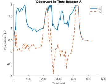
The observers are defined as ˆxG1:= z1− s1and ˆxG2:= z2−

s1− s2, each one of them converges to

∑

i∈G₁ 1 yi xiand

∑

i∈G₂ 1 yi xi,

respectively. A simulation of the observers trajectory can be seen from figure 2 where s1 and s2 were taken as sobs1 and

sobs₂ , respectively.

Fig. 2: Observer evolution for Reactor A using the measure-ments of s1 and s2.

E. Mixed Integer Program

A mixed integer program is presented in order to classify each OTU as AOB, NOB, or not determined by using observers ˆxG1 and ˆxG2 as inputs. The objective function is to

minimize the error defined as the difference of the observers

and

_∑

i∈Gj

1 yi

xifor j ∈ {1, 2} . Let n be the number of different

OTU identified, m the number of measurements, and tj the

time stamp of measurement j ∈ [m] . The variables to decide the classification are:

Variables:

• a∈ {0, 1}n_{: a}

i= 1 if OTU i is classified as AOB, 0

otherwise.

• b∈ {0, 1}n_{: b}

i= 1 if OTU i is classified as NOB, 0

otherwise.

• kA ∈ Rn

+: kiA> 0 if OTU i is classified as AOB, 0

otherwise. If kA_i > 0 then kA i = y−1i . • kB∈ Rn

+: kBi > 0 if OTU i is classified as NOB, 0

otherwise. If kB_i > 0 then kB i = y−1i .

• _{ε ∈ R}m₊: εj error associated to classification of AOB in

measurement j.

• _{η ∈ R}m₊ : ηj error associated to classification of NOB

in measurement j.

Parameters of the optimization problem are divided in data as presented in table I, and meta-parameters: yA_{re f}, yB

re f, δ , ma, Ma, mb, Mb, meaning that these parameters

come from prior knowledge to the experiment. All together they give bounds for the variables kB _{and k}A_.

Parameters of the Problem

• W ∈ Mn×m(R+) : Wi j= xi(tj). Column j contain the

concentration of each OTU at timestamp tj.

• s1(tj) ∈ R+ ∀ j ∈ [m] as defined in table I. • s2(tj) ∈ R+ ∀ j ∈ [m] :as defined in table I. • xˆG1(tj) ∈ R

+ _{∀ j ∈ [m] : Observer evaluated at}

• xˆG2(tj) ∈ R

+ _{∀ j ∈ [m] : Observer evaluated at}

times-tamps.

• yA_{re f}, yB_{re f}∈ R+: Literature reference value for yields of

AOB and NOB, respectively.

• δ ∈ (0, 1): fraction allowed to deviate from the reference yields.

• mA, MA∈ R+: lower and upper bounds for kAi,

respec-tively. mA:=

1

(1 + δ )yA_{re f}, MA:= 1 (1 − δ )yA_{re f}.

• mB, MB∈ R+: lower and upper bounds for kBi,

respec-tively. mB:= 1 (1 + δ )yB re f , MB:= 1 (1 − δ )yB re f .

In the numerical experiences, the reference yield for AOB is yA_{re f} = 0.147 [gr odm/grNH4+], and for the NOB is yBre f =

0.042 [gr odm/grNO2–] where odm stands for organic dry

matter [8].

Based on the former discussion the following constraints

are imposed. The notation W• j is used to represent the j-th

column of matrix W . Constraints:

• AOB mass error classification: The difference between

ˆ

xG1 and the assigned mass at each measurement is

bounded by ε .

−εj≤ W• j>kA− ˆxG1(tj) ≤ εj ∀ j ∈ [m]. (16)

• NOB mass error classification: The difference between

ˆ

xG2 and the assigned mass at each measurement is

bounded by η.

−ηj≤ W• j>kB− ˆxG2(tj) ≤ ηj ∀ j ∈ [m] (17)

• Each species can be classified in only one functional

group:

ai+ bi≤ 1 ∀i ∈ [n] (18)

• Linking constraint (Big-M Constraints): Activation of

kA_i or k_iBwhen ai or bi is active, respectively:

mAai≤ kiA≤ MAai ∀i ∈ [n] (19)

mBbi≤ kiB≤ MBbi ∀i ∈ [n] (20)

• Objective Function: The minimum of the norms of

vector ε and η.

kεk2_{+ kηk}2₌ m

∑

j=1

(η2_j+ ε2_j) (21)

The problem to be solved is: min m

∑

j=1 (η2j+ ε2j) s.t. (16), (17), (18), (19), (20) ε , η , ∈ Rm+ a, b ∈ {0, 1}n kA, kB∈ Rn + (MIQP)

The problem (MIQP) falls in the category of mixed integer quadratic programming, and it can be properly described in terms of the number of OTU (n) and the number of functional

groups (r), and the number of observations (m). Note that since if one considers one observer per functional group, the number of variables is calculated as 2 × n × r + 2 × m × r. The number of restrictions is calculated as 2 × m × r + 3 × n × r. This shows that the number of restrictions and variables grow linearly with the number of OTU (for fixed r).

III. RESULTS AND DISCUSSION

In all cases here presented the computing time was less than a second with zero optimality gap. The solver GUROBI was used within a Matlab interface. The computer was equipped with 8gb of RAM memory and Intel core i3-7100U CPU 2,40 GHz .

By varying δ the classification changes for certain OTU. The method always classifies 35 OTU in the same guild, which represent 87 % of the total biomass found. While 9 of them changed of class by varying the allowed bounds. Not all of the present OTU were participating in the nitri-fication process. This can be explained by the presence of heterotrophs which are feeding on decayed cell material and or predators.

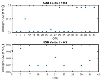
The obtained yields were plotted for the case δ = 0.3 in figure 3. One can see that the classification usually assigns the minimum or maximum yield.

Fig. 3: Obtained Yields for Reactor A

The study shows that the bounds imposed on the inverse of the yields (kA, kB) deserve some attention, since they can change the classification of some OTU. A more precise quan-tification of the possible variability within a guild escapes the authors’ knowledge. In the literature a measurement error of 30 % is usually found, therefore δ = 0.3 was taken in order to compare both reactors.

The results for the comparison of both reactors can be seen in Table II, were one notes that 3 OTU were assigned to a different functional group (highlighted in dark grey); it is very unlikely from a biological point of view that they had changed their function in each chemostat, implying that the classification can be tricked in certain cases. 15 OTU were assigned to a functional group in one case, but to

TABLE II: Comparison of Both Reactors and results of previous work.

A 1 under an AOB and NOB columns represent classification in the functional group, 0 means not classified in the functional group. Rows highlighted in light grey show OTU that changed from either AOB or NOB in one reactor to none in the other one. Rows highlighted in dark grey show OTU that changed from either AOB or NOB in one reactor to NOB or AOB, respectively, in the other one. Highlighted in light blue the cases where the classification changed from either AOB or NOB in one work to none in the other. Higlighted in blue the cases where classification changed from either AOB or NOB in one work to NOB or AOB in the other work, respectively. Time present in bold means it was close to clones identified in a database. ND stands for non demonstrated nitrifying capacity.

. Reactor A Reactor B Functional Assignment Functional Assignment OTU Relative Species

Abundance (%) _WorkThis Previous_Work

Relative Species

Abundance (%) _WorkThis Previous_Work Time

Present

(%) Mean Max AOB NOB AOB NOB

TimePresent

(%) _{Mean Max AOB NOB AOB NOB}

1 20 0 2 1 0 1 0 9 0 3 1 0 1 0 2 31 1 6 1 0 0 1 20 0 2 1 0 0 0 3 15 0 3 0 0 0 0 3 0 3 0 0 0 0 4 0 0 0 0 0 0 0 16 0 5 1 0 1 0 5 57 1 11 0 1 0 1 81 NOB 4 27 0 1 0 1 6 32 1 15 0 1 0 1 25 1 7 0 0 0 1 7 14 0 4 0 0 1 0 24 1 5 1 0 0 0 8 71 3 18 1 0 1 0 17 0 11 0 0 1 0 9 24 NOB 1 6 0 0 0 0 36 1 8 0 0 0 1 10 19 1 9 0 0 1 0 16 0 5 1 0 0 1 11 12 ND 0 13 0 0 1 0 10 0 7 0 0 0 0 12 19 1 8 1 0 1 0 6 0 9 1 0 1 0 13 31 1 12 0 0 0 1 88 2 8 0 1 0 1 14 36 ND 1 9 1 0 0 0 20 1 9 1 0 0 1 15 38 1 12 1 0 0 1 41 1 8 1 0 0 1 16 44 1 4 0 0 0 0 83 2 6 0 0 0 1 17 36 1 4 0 1 0 1 30 1 8 0 1 0 1 18 35 1 10 0 1 0 1 0 0 0 0 0 0 1 19 11 ND 0 4 0 1 0 1 20 0 3 0 0 0 0 20 19 0 3 1 0 0 1 31 1 5 1 0 1 0 21 41 1 6 0 1 0 1 18 0 4 0 1 0 0 22 15 0 2 0 1 0 1 31 1 7 0 1 0 1 23 73 ND 2 8 0 0 1 0 76 2 8 0 0 1 0 24 23 1 4 0 1 1 0 23 0 5 1 0 0 1 25 64 ND 2 11 1 0 1 0 89 3 18 1 0 1 0 26 34 1 5 1 0 0 1 17 0 4 1 0 1 0 27 18 1 12 1 0 0 1 40 3 23 1 0 0 0 28 41 1 7 0 0 1 0 28 1 13 0 0 1 0 29 45 ND 2 6 1 0 1 0 15 0 5 0 0 1 0 30 16 1 11 0 1 0 1 76 ND 2 10 1 0 0 1 31 23 1 5 1 0 0 1 20 1 13 1 0 0 1 32 60 2 18 1 0 0 1 58 1 6 0 1 0 1 33 50 2 36 1 0 1 0 95 4 49 1 0 1 0 34 17 1 16 0 1 0 0 0 0 0 0 0 0 0 35 100 ND 10 41 1 0 1 0 100 ND 12 38 1 0 1 0 36 50 3 26 1 0 1 0 96 5 28 0 0 1 0 37 100 ND 6 37 0 0 1 0 39 2 10 0 0 1 0 38 100 AOB 38 77 1 0 1 0 100 AOB 35 65 1 0 1 0 39 30 1 13 1 0 1 0 42 2 20 0 0 0 0 40 0 0 0 0 0 0 0 57 2 11 0 1 0 1 41 25 1 5 0 0 0 0 11 1 28 0 0 1 0 42 17 1 13 0 1 0 0 9 0 12 0 0 1 0 43 93 5 30 0 0 1 0 93 5 29 1 0 0 0 44 11 1 21 1 0 1 0 0 0 0 0 0 0 0

none in the other (highlighted in light grey); which can be explained by their low abundance and presence time in the reactors where they were not assigned to any guild. Finally 26 OTU were assigned to the same guild (highlighted in white), representing a mean abundance of 74 % and 76 % of the total biomass of reactors A and B, respectively. The mean abundance corresponding to AOB in reactors A and B was of 71 and 69 % and of the total biomass, respectively. while the abundance of the NOB community in reactors A and B was 9 and 11 % of the total biomass, respectively.

The method used in the work of Dumont et al.[1], con-sisted in generating the total AOB and NOB biomass from an observer. Then they randomly picked 10 OTU and tested all the possible assignments to find the one that best fitted the generated AOB and NOB biomasses. They repeated this process 10000 times and finally assigned probabilities to each OTU to be classified as either AOB, NOB or not determined. It took three days of computing time.

Comparison from the classification obtained from the previous work can be seen from table II as well. In Reactor A 19 OTU were classified differently, representing 27 % of the total biomass; 7 out of 19 OTU (highlighted in blue) changed functional group while the others (highlighted in light blue) had no functional group assigned in one of the works. In Reactor B, 23 OTU were classified differently, representing 32 % of the total biomass; 5 out of 23 OTU (highlighted in blue) changed functional group while the others (highlighted in light blue) had no functional group assigned in one of the works. The change in functional group (highlighted in blue) was systematically from AOB with the method here presented, to NOB from the previous work. Another point worth noting is that 7 and 9 false positives (assignment as AOB or NOB when database assigned ND) can be seen from this work and previous work, respectively. This suggests that one should consider modelling for heterotrophs, or taking out the rows corresponding to the ND from the mass Matrix W of problem (MIQP). The disagreement from the methods may be explained, partially, from the low relative abundances of the OTU which should create difficulties in any method.

Testing the effectiveness of the method would require chemostat experiments with a completely characterized in-oculum. However some a priori advantages of the method here presented are highlighted: (1) Allows a deviation from a reference yield accounting for variability within a microbial community, (2) the only user-defined parameter (δ ) is sug-gested from experimental error (3) all OTU can be compared at the same time, and (4) low computing time.

IV. CONCLUSIONS ANDPERSPECTIVES

The classification problem of assigning a functional group to the different microorganisms present in bioreactors was solved from an asymptotic observer that bypasses the choice of the growth function and mixed integer programming.

The extension of the method to other types of bioprocess is currently under development by considering the general invariants described in [11] and biological knowledge for the different functional groups interacting in the process. The

complexity of (MIQP) offers, at least theoretically, chances that the problem is solvable for a big number of OTU, if the number of functional groups remain low.

The use of mixed integer programming seems more suit-able as an engine for classification than testing combinations; it inherently handles the combinatorial nature of the task.

ACKNOWLEDGMENT

The authors thank GUROBI for the license to solve the MIQP. This work was supported by project Thermomic ANR-16-CE04-0003.

REFERENCES

[1] M. Dumont, A. Rapaport, J. Harmand, B. Benyahia, and J. J. Godon, “Observers for microbial ecology - how including molecular data into bioprocess modeling?” in 2008 Mediterranean Conference on Control and Automation - Conference Proceedings, MED’08, 2008. [2] S. Narayanasamy, E. E. Muller, A. R. Sheik, and P. Wilmes,

“Inte-grated omics for the identification of key functionalities in biological wastewater treatment microbial communities,” Microbial Biotechnol-ogy, 2015.

[3] S. Widder, R. J. Allen, T. Pfeiffer, T. P. Curtis, C. Wiuf, W. T. Sloan, O. X. Cordero, S. P. Brown, B. Momeni, W. Shou, H. Kettle, H. J. Flint, A. F. Haas, B. Laroche, J. U. Kreft, P. B. Rainey, S. Freilich, S. Schuster, K. Milferstedt, J. R. Van Der Meer, T. Grobkopf, J. Huisman, A. Free, C. Picioreanu, C. Quince, I. Klapper, S. Labarthe, B. F. Smets, H. Wang, O. S. Soyer, S. D. Allison, J. Chong, M. C. Lagomarsino, O. A. Croze, J. Hamelin, J. Harmand, R. Hoyle, T. T. Hwa, Q. Jin, D. R. Johnson, V. de Lorenzo, M. Mobilia, B. Murphy, F. Peaudecerf, J. I. Prosser, R. A. Quinn, M. Ralser, A. G. Smith, J. P. Steyer, N. Swainston, C. E. Tarnita, E. Trably, P. B. Warren, and P. Wilmes, “Challenges in microbial ecology: Building predictive understanding of community function and dynamics,” 2016. [4] M. J. Wade, J. Harmand, B. Benyahia, T. Bouchez, S. Chaillou,

B. Cloez, J.-J. Godon, C. Lobry, B. Moussa Boubjemaa, A. Rapaport, M. J. Wade, J. Harmand, B. Benyahia, T. Bouchez, S. Chaillou, B. Cloez, J.-J. Godon, B. Moussa Boudjemaa, A. Rapaport, T. Sari, R. Arditi, and C. Lobry, “Perspectives in Mathematical Modelling for Microbial Ecology,” Ecological Modelling, 2016.

[5] M. T. Madigan, J. M. Martinko, D. A. Stahl, and D. P. Clark, Brock Biology of Microorganisms, 13th Edition, 2012.

[6] M. Dumont, J. Harmand, A. Rapaport, and J. J. Godon, “Towards functional molecular fingerprints,” Environmental Microbiology, 2009. [7] E. H. Battley, R. L. Putnam, and J. Boerio-Goates, “Heat capacity measurements from 10 to 300 K and derived thermodynamic functions of lyophilized cells of Saccharomyces cerevisiae including the absolute entropy and the entropy of formation at 298.15 K,” Thermochimica Acta, vol. 298, no. 1-2, pp. 37–46, sep 1997. [Online]. Available: https://www.sciencedirect.com/science/article/pii/S0040603197001081 [8] U. Wiesmann, “Biological nitrogen removal from wastewater,”

Biotechnics/Wastewater, 1994.

[9] J. Harmand, C. Lobry, A. Rapaport, and T. Sari, The Chemostat: Mathematical Theory of Microorganism Cultures. John Wiley & Sons, 2017.

[10] K. V. Waller and P. M. M¨akil¨a, “Chemical Reaction Invariants and Variants and Their Use in Reactor Modeling, Simulation, and Control,” Industrial and Engineering Chemistry Process Design and Develop-ment, 1981.

[11] D. Dochain, “State and parameter estimation in chemical and bio-chemical processes: A tutorial,” Journal of Process Control, 2003.