Complexity and financial panics

MITLIBRARIES

DEWEY

_i]

He

21

'

W$

₃

_{9080 03317 5842}

Massachusetts

Institute

of

Technology

Department

of

Economics

Working

Paper

Series

Complexity

and

Financial Panics

Ricardo

J.

Caballero

Alp Simsek

Working

Paper 09-17

May

15.

2009

Revised June

17,2009

RoomE52-251

50

Memorial

Drive

Cambridge,

MA

02142

This

paper

can

be

downloaded

without

charge

from the

SocialScience Research

Network Paper

Collection at

Complexity

and

Financial

Panics

Ricardo

J.

Caballero

and

Alp

Simsek*

June

17,

2009

Abstract

During extreme financialcrises, all ofasudden, thefinancialworld thatwas once

rife with profit opportunities for financial institutions (banks, for short)

becomes

exceedingly complex. Confusion and uncertainty follow, ravaging financial markets

and triggeringmassiveflight-to-quality episodes. In this paper

we

proposea

model

ofthis

phenomenon.

In our model, banks normally collect information about their

trading partners which assures

them

of the soundness ofthese relationships.

How-ever,

when

acutefinancial distressemergesin partsofthe financialnetwork, it is not

enough to be informed about these partners, as it also

becomes

important to learn

about the health of their trading partners.

As

conditions continue to deteriorate,

banks

must

learn about the health of the trading partners of the trading partners

ofthe trading partners, and so on. At

some

point, thecost ofinformation gathering

becomes

too

unmanageable

for banks, uncertainty spikes, and they have no option but to withdraw from loan

commitments

and illiquid positions.

A

flight-to-quality

ensues, and the financial crisis spreads.

JEL

Codes:

E0. Gl, D8,

E5

Keywords:

Financial network, complexity, uncertainty, flight to quality,

cas-cades, crises, information cost, financial panic, credit crunch.

"MIT

and

NBER,

and MIT,respectively. Contact information: caball@mit.edu andalpstein@mit.edu.

We

thank Mathias Dewatripont, Pablo Kurlat, GuidoLorenzoni, Juan

Ocampo

and seminarparticipants

Digitized

by

the

Internet

Archive

in

2011

with

funding

from

Boston

Library

Consortium

Member

Libraries

1

Introduction

The

dramatic

rise in investors'

and

banks' perceived uncertainty is at the core of the

2007-2009

U.S. financial crisis. All of a sudden, a financial

world

that

was once

rife

with profit opportunities for financial institutions (banks, for short),

was

perceived to be

exceedingly complex.

Although

the

subprime shock was

small relative to the financial

institutions' capital,

banks

acted as if

most

of their counterparties

were

severely

exposed

to the

shock

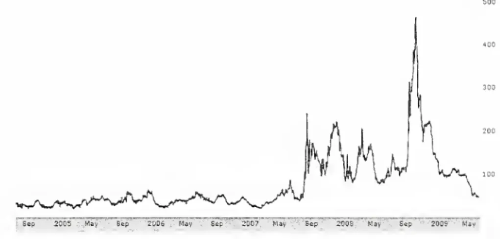
(seeFigure 1).

Confusion

and

uncertainty followed, triggering the worst case

of flight-to-quality that

we

have

seen in the U.S. since the

Great

Depression.

-^r-

6e

T

,oK . Hi,

»5^i55n

«

av .-sr-

5»nr.r

sir-Figure 1:

The

line corresponds to the

TED

spread in basis points (source:

Bloomberg),

the interest rate difference

between

the interbank loans (3

month

LIBOR)

and

the

US

government

debt (3

month

Treasury bills).

An

increase in the

TED

spread typically

reflects a higher perceived risk of default

on

interbank loans, that is,

an

increase in the

banks' perceptions of counterparty risk.

In this

paper

Ave present a

model

of the

sudden

rise in complexity, followed

by

wide-spread panic in the financial sector. In the model,

banks

normally collect, information

about

their direct trading partners

which

serves to assure

them

of the

soundness

of these

relationships.

However,

when

acute financial distress

emerges

in parts of the financial

network, it is not

enough

to be informed

about

these partners, but it also

becomes

impor-tant for the

banks

to learn

about

the health of their trading partners.

And

as conditions continue to deteriorate,

banks

must

learn

about

the health of the trading partners of the tradingpartners, oftheir trading partners,

and

so on.

At

some

point, the cost of

informa-tion gathering

becomes

too large

and

banks,

now

facing

enormous

uncertainty, choose to

withdraw

from

loan

commitments

and

illiquid positions.

A

flight-to-quality ensues,

and

the financial crisis spreads.

The

starting point ofour

framework

is a standard liquidity

model

where banks

(rep-resenting financial institutions

more

broadly) have bilateral linkages in order to insure

against local liquidity shocks.

The

whole

financial

system

is a

complex network

of

link-ages

which

functions

smoothly

in the

environments

that it is designed to handle,

even

though no

bank knows

with certainty all the

many

possible connections within the

net-work

(that is, each

bank knows

the identities ofthe other

banks

but not their exposures).

However,

these linkages

may

also

be

the source of contagion

when

an

unexpected

event

of financial distress arises

somewhere

in the network.

Our

point of departure

with

the

literature is that

we

use this contagion

mechanism

not as the

main

object of

study

but

as the source of confusion

and

financial panic.

During normal

times,

banks

only

need

to

understand

the financial health of their neighbors,

which

they can learn at low cost. In contrast,

when

a significant

problem

arises in parts of the

network

and

the possibility of

cascades arises, the

number

of

nodes

to

be

audited

by

each

bank

rises since it is possible that theshock

may

spread to the bank's counterparties. Eventuallythe

problem

becomes

too

complex

for

them

to fully figure out,

which

means

that

banks

now

face significant

uncertainty

and

they react to it

by

retrenching into liquidity-conservation

mode.

This

paper

is related to several strands of literature.

There

is

an

extensive literature that highlights the possibility of

network

failures

and

contagion in financial markets.

An

incomplete list includes Allen

and Gale

(2000),

Lagunoff

and

Schreft (2000),

Rochet

and

Tirole (1996), Freixas, Parigi

and Rochet

(2000), Leitner (2005), Eisenberg

and

Noe

(2001), Cifuentes, Ferucci

and

Shin (2005) (see Allen

and

Babus

(2008) for a recent survey).

These

papers focus

mainly

on

the

mechanisms

by

which

solvency

and

liquidity

shocks

may

cascade

through

the financial network. In contrast,

we

take these

phenomena

as the reason for the rise in the complexity of the

environment

in

which

banks

make

their decisions,

and

focus

on

the effect of this complexity

on

banks' prudential actions.

In this sense, our

paper

is related to the literature

on

flight-to-quality

and Knightian

uncertainty in financial markets, as in Caballero

and

Krishnamurthy

(2008),

Routledge

and

Zin (2004)

and

Easley

and

O'Hara

(2005);

and

also to the related literature that

investigates the effect of

new

events

and

innovations in financial markets, e.g. Liu, Pan,

and

Wang

(2005),

Brock

and

Manski

(2008)

and Simsek

(2009).

Our

contribution relative

tothisliteratureisinendogenizing therise inuncertainty

from

thebehavior ofthefinancial

network

itself.

More

broadly, this

paper

belongs to

an

extensive literature

on

flight-to-quality

and

financial crises that highlights theconnection

between

panics

and

a decline in

the financialsystem's ability tochannel resources tothe real

economy

(see, e.g., Caballero

and

Kurlat (2008), for asurvey).

network

and

describe a rare event as a perturbation to the structure of banks' shocks.

Specifically,

one

bank

suffers

an

unfamiliarliquidity

shock

for

which

it

was

unprepared.

We

next

show

thatif

banks

can costlesslygatherinformation

about

the

network

structure, the

spreadingofthisshock into precautionary responses

by

other

banks

istypically contained.

This

scenario

with no network

uncertainty is the

benchmark

for our

main

results

and

is similar (although with

an

interior equilibrium) to Allen

and Gale

(2000).

Our

main

contribution is in Section 3,

where

we

make

information gathering costly. In

thiscontext, ifthe cascadeissmall, either because theliquidity

shock

is limited or

because

banks' buffers are significant,

banks

are able to gather the information they

need

about

their indirect

exposure

totheliquidity

shock

and

we

are

back

to thefullinformation results of Section 2.

However,

once cascades are large enough,

banks

are unable to collect the information they

need

torule out a severe indirect hit. Their response to this uncertainty

is to

hoard

liquidity

and

to retrench

on

their lending,

which

triggers a credit crunch. In

Section 4

we show

that

under

certain conditions, the response in Section 3

can

be

so

extreme, that the entire financial

system

can collapse as a result of the flight to quality.

The

paper

concludes

with

a final

remarks

section

and

several appendices.

2

The

Environment

and

a

Free-Information

Bench-mark

In this section

we

first introduce the

environment

and

the characteristics ofthe financial

network

along

with

a

shock which was

unanticipated at the

network

formation stage (i.e.

the financial

network

was

not designed to deal with this shock).

We

next characterize

the equilibrium for a

benchmark

case in

which

information gathering is free so that the

market

participants

know

the financial network.

2.1

The

Environment

There

arethree dates{0. 1,2}.

There

isasingle

good

(onedollar) that serves asnumeraire,

which

can

be

kept in liquid reserves or it can be loaned to production firms. If kept in

liquid reserves, a unit of the

good

yields one unit in the next date. Instead, if a unit

is loaned to firms at date 0, it then yields

R

>

1 units at date 2 if it is not

unloaded

before this date.

At

date 1, the lender can

unload

the loan (e.g.

by

settling it

with

the

borrower

at a discount)

and

receive r

<

1 units.

To

simplify the notation,

we assume

r

%

throughout

this paper.

Banks

and

Their

Liquidity

Needs

The

economy

has

2n continuums

of

banks denoted

by

{b3_{}~_}

1

.

Each

of these

continuums

is

composed

of identical

banks

and, for simplicity,

we

refer to each

continuum

b3 _as

_bank

b3

,

which

is our unit ofanalysis.

1

Each

bank

b3 _{has initial assets}

_which

consist of y units of liquid reserves set aside for liquidity

payments,

fjo

<

I

—

y units offlexible reserves set

aside for

making new

loans at date (but

which can

also

be

hoarded

as liquid reserves)

and

1

—

y

—

yo units ofloans.

The

bank's liabilities consist of a

measure one

of

demand

deposit contracts.

A

demand

deposit contract pays l

}

>

1 at date 1 if the depositor is

hit

by

a liquidity shock

and

^

>

h at date 2 if the depositor is not hit

by

a liquidity

shock. Let

u

3

_€

[0, 1]

be

the

measure

of liquidity-driven depositors of

bank

b3 (i.e. the

size ofthe liquidity

shock

experienced

by

the bank),

which

takes

one

of the three values

in {<Z\u_L,u

_H

} with uj

_h

>

lo_l

and

u>

=

(u>

_H

+

ui_L

) /2,

and suppose

y

—

l\(I)

and

₍₁

—

_y)

R

=

1_{2 Cj.}

Note

that, if the size of the liquidity shock is Cu, the

bank

that loans all of its flexible

reserves j/n at date has assets just

enough

to

pay

l\ (resp. U) to earl}' (resp. late)

depositors.

The

central trade-off in this

economy

will

be

whether

the

bank

will loan its

flexible reserves _yo (which it set aside for this purpose) or

whether

it will

hoard

some

of

this liquidity as aprecautionary response to a rare event that

we

describe below.

The

Financial

Network

The

liquidityneeds atdate 1

may

not

be

evenlydistributed

among

banks,

which

highlights

one

ofthe (man}') reasons for an interlinked financial network. Moreover, the

main

source

of complexity later

on

will

be

confusion about the linkages

between

different banks.

To

capturethispossibility

we

leti

E

_{1, .., 2ra} denote slots in afinancial

network

and

consider

a

permutation

p : {1. ..,

2n}

—

> _{1, ..,

2n}

that assigns

bank

bp

^

to slot i.

We

consider a

financial

network

denoted

by:

b

(p)

=

(b

p(1) _{-> 6"}(2) _->

^

(3)

-.... -» bp

W

^

6P(i)) ) (!)

where

the arc

—

» denotes that the

bank

in slot ? (i.e.,

bank

bp{

-l)

) has a

demand

deposit in

the

bank

in the

subsequent

slot i

+

1 (i.e.,

bank

bp^+l) ) equal to

z

=

(Q-u

_L), (2)

where

we

use

modulo

2n

arithmetic for the slot index i 2

We

refer to

bank

6p('+1

) as the

forward

neighbor of

bank

bp

^

(and similarly, to

bank

bp^l) _{as the}

backward neighbor

_of

bank

fr^!+1)

).

The

possibility ofconfusionarises later

on from banks

knowing

the identity

ofother

banks

but not their particular linkages (i.e., the actual

permutation

p).

As

we

formally describe in

Appendix

A.l (and similar to Allen-Gale (2000)), in the

normal

environment, the financial

network

facilitates liquidity insurance

and

enables

liq-uidity to flow

from

banks

that experience a low liquidity shock (uj_l) to the

banks

that

experience a high liquidityshock (w

_w

). even

when

the financial

network

b

[p) is

unknown

to the banks.

Our

focus is

on

the effect of the financial interlinkages in case of

an

unan-ticipated shock for

which

the financial

network

is not necessarily designed for,

which

we

describe next.

A

Rare Event

At

date the

banks

learn that all

banks

will experience the average liquidity

shock

uj at

date 1, however, theyalso learn thatone bank, b3,

becomes

distressed

and

loses 6

<

y ofits

liquid assets.

As we

formally

demonstrate

below, thelosses inthedistressed

bank

b3

_might

spill over to the other

banks

viathe financial

network

b

_[p), thus the banks'

knowledge

of

thefinancial

network

ispotentiallypayoffrelevant. In particular, this

knowledge

influences

whether

the

banks

use the flexiblereserves j/n to

make

new

loans or to

hoard

liquidity.

We

are thus lead to describe the central feature of our model: the banks' uncertainty about the financial

network

b

(p).

Network

Uncertainty

and

Auditing

Technology

We

let

B =

{b

_(p) | p

: {1,..,

2n}

—

> _{{1, ,.,2n}} is a

permutation}

. (3)

denote the set of possible financial networks.

Each

bank

b3 _observes

its slot i

=

p~

l

(j)

and

the identities ofthe

banks

in its neighboring slots i

—

1

and

i

+

1. This information

narrows

down

the potential

networks

to the set:

B

3

(p)=

(h{p)<EB

p(i-l)

=

p(i-l)

p(i)

=

p(i) I p(i

+

l)

=

p(i

+

l) ,

where

i

=

p l (j)

-In particular, i represents the slot with index i' £ {l,...2n} that is the modulo In equivalent of

Figure 2:

The

financial

network

and

uncertainty.

The

bottom-left

box

displays the

actual financial network.

Each

circle corresponds to aslot inthe financial network,

and

in

this realization ofthe network, each slot i contains

bank

b1 (i.e. _p(i)

=

i).

The

remaining

boxes

show

the other

networks

that

bank

61 finds plausible after observing its neighbors (i.e. the set

B

l _(p)).

Bank

bl cannot tell

how

the

banks

{b5.b4,b5

} are ordered in slots {3.4.5}.

are

Note

that the

bank

b3 _{does not}

_know

_how

_{the remaining}

_banks

_(V)-*,,^^

,

{, „/i+x)\

assigned to the

remaining

slots (see Figure 2). In particular, each

bank

b3

^

b3

_knows

that the

bank

b3 _{is distressed, but it does not necessarily}

_know

_{the slot}

i=P~

l

Q)

ofthe distressed bank.

This

is key, since it

means

that a bank b3

^

_b3 _{does not necessarily}

know

how

jar

removed

it is

from

the distressed bank.

Each bank

b3 _{can acquire}

_more

_information

_about

_{the financial}

_{network through an}

auditing technology.

At

date 0, a

bank

b3 _{in slot i (i.e. with}

j

=

p(i)) can exert effort

to audit its forward neighbor 6p(i+1' _in order to learn the identity of_this bank's

forward

neighbor bp(-'^2^

.

Continuing

this way, a

bank

V

that audits a

number,

a

3

, of

balance

sheets learns the identity ofits a3

₊

_{1 forward neighbors}

_{and narrows}

_{the set ofpotential}

financial

networks

to: B> (p | a 3 )

=

{

b

(p)

£

B

p(i-l)

=

p(i-l)

_ p{i

+

a 3

₊

₁₎

=

_p(t

+

_a3

₊

1) ,

where

i

=

p _(j)

We

denote the posterior beliefs of

bank

b3

with f

3 (. | p,a

3

)

which

has support

equal

to

B

3

(p.a3) given assumption:

Assumption

(FS).

Each

bank

has a prior belief

_f

3

(.) over

B

with full support.

In the

example

illustrated inFigure 2, if

bank

b1 auditsone balancesheet, thenit

would

learn that

bank

b3 is assigned to slot 3

and

it

would narrow

down

the set of

networks

to the

two

boxes at the left

hand

side ofthe

bottom

row

in Figure 2.

Bank

Preferences

and

Equilibrium

Consider a

bank

b3

_and

_{denote the bank's actual}

_payments

_{to early}

_and

_{late depositors}

by

q\

and

qi (which

may

in principle be different

than

the contracted values l^

and

/₂).

Because

banks

are infinitesimal, they

make

decisions taking the

payments

of the

other

banks

as given.

The

bank makes

the audit

and

liquidity hoarding decisions, a3

_E

{0,1.,..,277

—

3}

and

y

3

E

[0,yo], at date (equivalently, j/o

—

y

J

E

<0,j/oi denotes the

number

of

new

loansthe

bank makes

at date 0).

At

date 1, the

bank

chooses to

withdraw

some

ofits depositsin the neighbor bank,

which

we

denote

by

z3

_E

[0, z],

and

it

may

also

unload

some

of its outstanding loans.

The

bank

makes

these decisions to

maximize

_q\

until it can

meet

its liquidity obligations to depositors, that is, until _q\

=

l\. Increasing

q\

beyond

l\ has

no

benefit for the bank, thus once it satisfies its liquidity obligations, it

then

tries to

maximize

the return to the late depositors q\.

We

capture this behavior with the following objective function

«(lW</i}g{' +

lW>Zi}^)-d(aO

(4)

where

v :

R+

—

>

K

₊₊

is a strictly concave

and

strictly increasing function

and

d(.) is

an

increasing

and convex

function

which

captures the bank's

non-monetary

disutility

from

auditing.

When

the

bank

b3

is

making

adecision that

would

lead to

an

uncertain

outcome

for _(qi^qi) (which will be the case in Section 3), then it

maximizes

theexpectation of

the

expression in ₍₄₎ given its posterior beliefs

_f

J

(. | p,

a3

).

Suppose

that the depositors' early/late liquidity shocks are observable,

and

a

bank

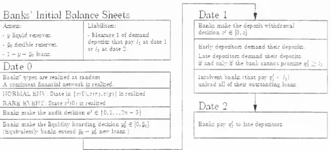
Banks'

Initial

Balance

Sheets

Assets: Liabilities:

- _yliquid reserves

- Date 1 paymentto early

depositors: Dl^ =_y

- yo tiexiblereserves

- Date 2 pavmenttolate

- 1—y—po loans. depositors: Qlz

=

(1—y)R

- j demand depodtsin - ? demand deposit:neld by

forward neighborbank backward neighborbank.

Date

Bankslearn that

- Eachwillhave shod;u> frerlected onabove balancesheetcl.

- Ba.nkb1 _{becomesdistressed and loses 8 liquid reserves}

Banksmakethe audit dedsiona1 ₆

{0,1, 3}.

Banksmoke theliquidity hoardingdecidony'€ [0,§ ]

(Equivalent!}-banks extend y — y^new loans,)

Date

1

Banksmoke thedepodtwithdrawal

dedsion ,-; _{e [0,;j.}

Earlydepodtorsdemand their deposits

Late depodtorsdemand tneirdeposits

ifand onlyifthe bo.nl;cannot promise ql

Insolvent banks (thatpay q{ < /]!

unload allof theiroutstandingloans

Date

2

Bankspayqi to la,tedepodtors.

Figure 3: Timeline of events.

depositors if they arrive early.3

With

this assumption, the continuation equilibrium for

bank

V

at date 1 takes

one

of

two

forms. Either there is a no-liquidation equilibrium in

which

the

bank

is solvent

and

pays

q{

=

li,q

3

2

>k,

(5)

while the late depositors

withdraw

at date 2; or there is a liquidation equilibrium in

which

the

bank

is insolvent, unloads all outstanding loans,

and

pays

q{

<

l

u

4

=

0, (6)

while all depositors (including the late depositors)

draw

their deposits at date 1.

Figure 3 recaps the timeline of events in this

economy.

We

formally define the

equi-librium as follows.

Definition

1.

The

equilibrium, is a collection ofbank auditing, liquidity hoarding, deposit

withdrawal,

and

payment

decisions

{a^p),yi(p)

)

^(p),ql(p),q

J

2 (p)}_j

such

that,

b(p)£B

given the realization of the financial

network

b

(p)

and

the rare event, each bank b3

maxi-3_Without

this assumption, therecould bemultiple equilibria for latedepositors'early/latewithdrawal

decisions. In cases with multiple equilibria, this assumption selects the equilibrium in which no late

raizes expected utility in (4) according to its prior belief

_f

J

(.) over B, the insolvent

banks

(with _{q\ (p)}

<

l\) unload all of their outstanding loans at date 1

and

the late depositors

withdraw

deposits early if

and

only ifq^ (p)

<

l\ _(cf. Eqs. (5)

and

{&)).

We

next turn to the characterization of equilibrium.

Note

that for each financial

network

b

(p)

and

for each

bank

b3, thereexists a unique k

G

{0, ..,

2n

—

1} such that

j

=

p(i-

k)

,

which

we

define as the distance of

bank

b3

_from

_{the distressed bank.}

_{As we}

will see,

the distance k will

be

the payoff relevant information for a

bank

b3 _{that decides}

_how

much

liquidity to

hoard

at date since it will determine

whether

or not the crisis that

originates at the distressed

bank

b3 _{will cascade to}

_bank

_b3

.

The

banks

b

p^~l

\bp

^

, b

p(-l+1

\

respectivelywith distances 1,

and 2n

—

1,

know

their distances,

but

the remaining

banks

(with distances k

€

{2. ...2n

—

_2})

do

not have this information a priori

and

they assign a

positive probability toeach k

£

{2, ..,

2n

—

2} (they rule out k e {1,2n

-

1} by observing

their forward

and backwards

neighbors). Note, however, that the

bank

b3 can use the auditing technology to learn

about

the financial

network

and, in particular,

about

its

distance

from

the distressed bank.

A

bank

bp

^~

h' (with distance k) that audits a3

>

₁

banks

either learns its distance k (if k

<

a?.+ 1) or it learns that k

>

a3

₊

2.

In the

remaining

half of this section,

we

characterize the equilibrium in a

benchmark

case in

which

auditing is free so each

bank

learns its distance

from

the distressed

bank.

In subsequent sections,

we

characterize the equilibrium with costly audit

and

compare

it

with

the free-information

benchmark.

2.2

Free-Information

Benchmark

We

first describe a

benchmark

case in

which

auditing is free so each

bank

bp^x

~_k

>

chooses

full auditing ap^~k}

₌

2n

—

3. In this context

banks

learn the

whole

financial

network

b

(p) and, in particular, their distances.

At

date all

banks

anticipate receivinga liquidityshock, Co, at date 1

and

have liquid reserves equal to y

—

CjIi _{(plus y} offlexiblereserves), except for

bank

b3

=

6p(i'

which has

liquid reserves y

—

9.

At

date 1, the distressed

bank

bp

^

withdraws

its deposits

from the

forward neighbor bank.

As we show

in

Appendix

A.2, this triggers further

withdrawals

until, in equilibrium, all cross deposits are

withdrawn.

That

is

In particular,

bank

bp

^

tries, but cannot, obtain

any

net liquidity

through

cross

with-drawals.

The bank

also cannot obtain

any

liquidity by unloadingthe loans at date 1, since

each unit of

unloaded

loan yields r

«

0. Anticipating that it will not

be

able to obtain

additional liquidity at date 1, the distressed

bank

bp

^

hoards

some

its flexible _{reserves y}

by

cutting

new

loans at date in order to

meet

its liquidity

demand

at date 1. In order to

promise

late depositors at least /

l5 a

bank

with

no

liquid reserves left at

the

end

ofdate 1

must

have

at least

i-y-g.Ozm

(8)

units ofloans.

The

level _yj is a natural limit

on

a bank's liquidity hoarding (which plans

to deplete all ofits liquidity at date 1) since

any

choice

above

this

would

make

the

bank

necessarily insolvent. Ifthe

amount

offlexible reserves _y"oisgreater

than

_yj. then the

bank

can

hoard

at

most

_y"o of the flexible reserves while

remaining

solvent; or else it can

hoard

all ofthe flexible reserves yo-

Combining

the

two

cases, a bank's buffer is given

by

j3

=

min

_{j/o,yo} •

A

bank

can

accommodate

losses in liquidreserves

up

tothebuffer3, but

becomes

insolvent

when

losses are

beyond

3. It follows that the distressed

bank

6p(l) will be insolvent

whenever

>

P, (9)

that is,

whenever

its losses in liquid reserves are greater

than

its buffer.

Suppose

this is

the case so

bank

6/,(l) is insolvent. Anticipating insolvency, this

bank

will

hoard

as

much

liquidity as it can _y$

=

_y"o (since it

maximizes

_ql )

and

unloads all remaining loans at

date 1. Since the

bank

is insolvent, all depositors (including late depositors) arrive early

and

the

bank

pays

where

recall that _gf denotes

bank

6^'+1

''s

payment

to early depositors (whichis

equal

to /] if

bank

bp(l+l) is solvent).

Partial

Cascades.

Since

bank

bp

^

is insolvent, its

backward

neighbor

bank

bp

^~

l> will

experience losses in its cross deposit holdings, which, if severe enough,

may

cause

bank

£,p(i-!)-s insolvency.

Once

the crisis cascades to

bank

bp(-l

~l

\

it

may

then similarly

cascade

to

bank

bp<~'~ 2\ continuing its cascade

through

the

network

in this fashion.

We

conjecture that,

under

appropriate parametric conditions, thereexists athreshold

K

€

{1,..,2n

—

2} such that all

banks with

distance k

<

K

—

1 are insolvent (there are

K

such banks) while the

banks with

distance k

>

K

remain

solvent. In other words, the

crisis will partially cascade

through

the

network

but will be contained after

K

<

2n

—

2

banks have

failed.

We

refer to

K

as the cascade size.

Under

this conjecture,

bank

bp^ +1

\ which

has a distance

2n

—

1, is solvent.

Therefore

q

p(-'

=

/:

and

cfi in Eq. (10) can

be

calculated explicitly. Consider

now

the

bank

^p(r-i)

^,'i-j-j distance 1

from

the distressed bank.

To

remain

solvent, this

bank needs

to

pay

l\

on

its deposits to

bank

6p('_2)

but it receives only _qp

<

/]

on

its deposits

from

the

distressed

bank

bpl<L\ so it loses z il\

—

_qp j in cross-deposits. Hence,

bank

b

pl-L

~l>

will

also

go bankrupt

if

and

only if its losses

from

cross-deposits are greater than its buffer,

'i

—

*?i )

>

^i

w

hich can be rewritten as

qf

]

<h--z

- (11)

Ifthis condition fails, then the onlyinsolvent

bank

isthe original distressed

bank

and

the

cascade size is

K

=

1. If this condition holds, then

bank

bpii

~1

^ _{anticipates insolvency, it}

will

hoard

as

much

liquidity as it can, i.e. j/q

=

y

and

it will

pay

all depositors

•T"

-

/

(O

-

!+*£*?..

(12,

From

thispoint onwards, a pattern emerges.

The

payment

by an

insolvent

bank

{/,(, ~fc) (with k

>

1) is given

by

qf-k)

=

f

(qf-{k-']) )

and

thisbank's

backward

neighborbp^~^k+l^ isalso insolvent if

and

only if_q

p

'

<

lj

—

-.

Hence, the

payments

of the insolvent

banks

converge to the fixed point of the function

/(.) given

by

y -f _y ,

and

if

Q

y

+

yo

>

h

—

, (13) 'J

Ifcondition (13) fails, then the sequence lq^'

=

f (qp '

))

always remains below li

—

-,

andit can be checked that there is a full cascade, i.e. all banks are insolvent.

then (under Eq. (11)) there exists a unique

K

>

2 such that

qf'

k)

<h--

for each k

e

{0. ...

K

-

2} (14) , p{T-(K-\)) . ,

8

and

<7j

>

m

•

If

2n

—

2 is greater

than

the solution, A', to this equation, i.e. if

2n

-

2

>

A', ₍₁₅₎

then, Eq. (14)

shows

that (in addition to the trigger-distressed

bank

6p(!)) all

banks

bp(L ~k

) with distance k 6 _{1,...A'

—

1} are insolvent since their losses

from

cross de-posits are greater

than

their corresponding buffers. In contrast,

bank

bp(l~ h) (that

re-ceives _qp

from

its forward neighbor) is solvent, since it can

meet

its losses

from

cross deposits

by

hoarding

some

liquidity while still promising the late depositors at

least

_h

(i.e.

_qf~

K)

>

h). Since

bank

bp{J- K) is solvent, all

banks

bp{T

-k)

with

dis-tance k

6

{K

+

l,..,2n

—

1} are also solvent since they

do

not incur losses in cross-deposits.

Hence

these

banks do

not

hoard

any

liquidity, j/q

=

0,

and

they

pay

(<7i

=

h,<J

P

_~

^2)i verifying our conjecture for a partial cascade ofsize

K

under

conditions (13)

and

(15).

Sinceourgoal is tostudy the roleof

network

uncertainty in generating acredit crunch,

we

take the partial cascades as the

benchmark.

The

next proposition

summarizes

the

above

discussion

and

also characterizes the aggregate level of liquidity hoarding,

which

we

use as a

benchmark

in subsequent sections.

Proposition

1.

Suppose

the financial

network

is realized as b(p), auditing is free,

and

conditions (9), (13)

and

(15) hold.

For

a given financial

network

b(p), let J

=

p~

l (j)

denote the slot ofthe distressed bank.

(i)

For

the continuation equilibrium (at date I):

The

banks' equilibrium

payments

(9i

•

?2 ) are (weakly) increasing withrespect to their distance k

from

the distressed

bank

and

there is a partial cascade ofsize

K

<

2n

—

2

where

K

is defined by Eq. (14).

In particular, banks {frp(t

~^},

n (with distance

from

the distressed bank k

<

A'

—

I) are insolvent while the

remaining

banks {bpi-'~k

^} (with distance k

>

K)

are solvent.

(ii)

For

theex-ante equilibrium (at date0):

Banks

{bp

^~

k'

>

},_

n hoard as

much

liquidity as they can

and

unload all _of their existing loans at date 1, while banks {i>p(t

~fc)

}

do not hoard

any

liquidity or unload

any

loans.

Bank

bp<"L

~_h

^ hoards a _{level of liquidity}

j/q

!

=

z (l\

—

_q

p

'

)

which

is just

enough

to

meet

its losses

from

cross deposits (and does not unload

any

loans).

5r 4 -3 -2 -1 • O1

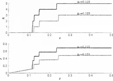
-08 o.e fa.04 0.2 0.2 _kr=!L122_ l7n=n,llfl _i*)=a.,iz3_ 1 0.2 04

Figure 4:

The

free-

information

benchmark.

The

top figure plots the cascade size

K

as a function of the losses in the originating

bank

9, for different levels ofthe flexible

reserves y~o.

The bottom

figure plots the aggregate level ofliquidity hoarding, !F, for the

same

set of {y~o}.

The

aggregate level ofliquidity hoarding is:

T

_{- 5Z}

yo

=

K

vo

+

yo

{L~ _A')

(16)

Discussion.

Proposition 1

shows

that,

under

appropriate parametric conditions, the equilibrium features a partial cascade

and

the aggregate level of liquidity hoarding, J-',

is roughly linear in the size of the cascade

K

(and is roughly continuous in 0).

Figure

4

demonstrates

this result for particular parameterization of the model.

The

top panel of the figure plots the cascade size

K

as a function of the losses in

the originating

bank

9 for different levels of the flexible reserves j/o- This plot

shows

that the cascade size is increasing in the level of losses 6

and

decreasing in the level of

flexible _{reserves y} . Intuitively, with a higher 9

and

a lower y , there are

more

losses to

be

contained

and

the

banks have

less

emergency

reserves to counter these losses,

thus

increasing the spread of insolvency.

The

bottom

panel plotstheaggregate levelofliquidityhoarding

JF

which

isa

measure

ofthe severity ofthe creditcrunch, asafunction of9. Thisplot

shows

that

T

alsoincreases

with

9

and

falls

with

_y . This is

an

intuitive result: In the free-information

benchmark

only the insolvent

banks

(and

one

transition

bank)

hoard

liquidity, thus the

more banks

are insolvent (i.e. the greater

K)

the

more

liquidity is

hoarded

in the aggregate.

Note

also that

T

increases "smoothly" with 9.

These

results offer a

benchmark

for the next sections.

There

we show

that once

audit-ing

becomes

costly,

both

A'

and

T

may

be

non-monotonic

in _y anc

h

more

importantly,

can

jump

with small increases in 9

.

3

Endogenous

Complexity

and

the

Credit

Crunch

We

have

now

laid out the foundation for our

main

result. In this section

we add

the

realistic

assumption

that auditing is costly

and demonstrate

that a massive credit

crunch

can arise in responseto

an

endogenous

increase in complexity

once

a

bank

in the

network

is sufficiently distressed. In other words,

when

A" is large, it

becomes

too costly for

banks

to figure out their indirect exposure. This

means

that their perceived uncertainty rises

and

they eventually

respond

bj' hoarding liquidity as a precautionary

measure

(i.e.,

T

spikes).

Note

that, unlike inSection 2.2,

we

cannot

simplify the analysis

by

solvingthe

equilib-rium

for a particular financial

network

b

_(p) in isolation, since, even

when

the realization

of the financial

network

is b(p), each

bank

also assigns a positive probability to other

financial networks

b

(p) 6 B.

As

such, for a consistent analysis

we

must

describe the

equilibrium for

any

realization ofthe financial

network

b

(p)

£

B

(cf. Definition 1).

Solving this

problem

in full generality is

cumbersome

but

we make

assumptions

on

the

form

of the

adjustment

cost function, the banks' objective function,

and on

the level

of flexible reserves, that help simplify the exposition. First,

we

consider a

convex

and

increasing cost function d(.) that satisfies

d{l)

=

and

d(2)>v(l

1

+

l2

)-v(0).

(17)

This

means

that

banks

can audit one balance sheet for free but it is very costly to audit

the second balance sheet. In particular, given the bank's preferences in (4), the

bank

will

never choose to audit the second balance sheet

and

thus each

bank

audits exactly

one

balance sheet, {a3 _(p)

=

1} .

Given

these audit decisions

and

the actual financial

L JJb(P)e/3

network

b

(p), a

bank

IP has a posterior belief

_f

J _{{.\p,l) with support}

_B

J

(p,l),

which

is

the set of financial

networks

in

which

the

bank

j

knows

the identities of its

neighbors

and

its second forward neighbor. In particular, the

bank

6p('~2) _learns

its distance

from

the distressed

bank

bp(l) (in addition to

banks

6pl' 1)

,6

p(l>

,6

p(,+1)

which

already

have

this

information

from

the outset).

We

denote the set of

banks

that

know

the slot of

the

distressed

bank

(and thus their distance

from

this

bank) by

B

know (p)

=

{b p^-2

\b

p(I-l) .bp{1),bp{T+l) } .

On

the other hand, each

bank

&^'-,c

> with k

6

{3,..,2n-2}

learns that _its distance

is at least 3 (i.e. k

>

3), but otherwise assigns a probability in (0. 1) to all distances

k

6

{3. ... 2n

—

2}.

We

denote the set of

banks

that are uncertain

about

their distance

by

^uncertain i \

_

np(r-3) ^p(T-4) ^p(J-{2n-2))\

Second,

we

assume

that the preference function v(.) in (4) is Leontieff v (x)

=

(xl~a

—

1) / (1

—

a) with

a

—

> oo, so that the bank's objective is:

mm

(1 {q{ (p)

<

h}

q{ (p)

+

1

{^

(p)

>

I,} qi (p))

-

d {a? (p)) . (18)

b(p)£BJ(p,l)

This

means

that

banks

evaluate their decisions according to the worst possible

network

realization, b(p),

which

they find plausible.

The

third

and

last

assumption

is that

yo

<

PS- (19)

That

is, the

bank

has less flexible reserves

than

the natural limit

on

liquidity

hoarding

defined in Eq. (8) (which also implies that the buffer is given by

3

=

_j/o)- This condition ensures that, in the continuation equilibrium at date 1. the

banks

that have

enough

liquidity are also solvent (since,

no matter

how much

of their flexible reserves they hoard,

they

have

enough

loans to

pay

the late depositors at least l\ at date 2).

We

drop

this

condition in the next section.

We

next turn to the characterization of the equilibrium

under

these simplifying

as-sumptions.

The

banks

make

their liquidity hoarding decision at date

and

deposit with-drawal decision at date 1

under

uncertainty (before their date 1 losses

from

cross-deposits

are realized).

At

date 1 the distressed

bank

bp^x)

withdraws

_{its deposits}

_from

_the

forward

neighbor

which

leads to the

withdrawal

of all cross deposits (see Eq. (7)

and

Appendix

A.2) as in the free-information

benchmark.

Thus, for

any

distressed bank, the only

way

to obtain additional liquidity at date 1 is

through

hoarding liquidity at date 0,

which

we

characterize next.

A

Sufficient Statistic for

Liquidity

Hoarding.

Consider a

bank

bp^~k) other

than

the original distressed

bank

(i.e.. A;

>

0).

A

sufficient statistic for this

bank

to

make

the' liquidity hoarding decision is _qp

''

(p)

<

li,

which

is the

amount

it receives in equilibrium

from

its

forward

neighbor. In other words, to decide

how much

of its flexible

reserves to hoard, this

bank

only needs to

know

whether

(and

how

much)

it will lose in cross-deposits. For example, if it

knows

with certainty that _qp _(p)

=

li (i.e. its

forward neighbor is solvent), then it hoards

no

liquidity, i.e. _y^ '

=

0. Ifit

knows

with

certainty that _qp _(p)

<

li

—

fi/z (i.e. its forward neighbor will

pay

so littlethat this

bank

will also

be

insolvent), then it hoards as

much

liquidity as it can, i.e. _y^

=

_y .

More

generally, if the

bank

bp^~k) hoards

some

y'

_G

[0,j/o] at date

and

its

forward

neighbor pays

x

=

_qP '

(p) &t date 1, then this bank's

payment

can be written as

qf-k)

{p)

=

q,\y'(y x}

and

qf

~k}

(p)

=

q2 [y',x], (20)

where

the functions qi[y',x]

and

cj2[y'..x] are characterized in Eqs. (26)

and

(27) in

Appendix

A.2.

At

date 0, the

bank

does not necessarily

know

x

—

_q

p

(p)

and

it

has to choose the level ofliquidity hoarding

under

uncertainty.

The

characterization in

Appendix

A.2 also

shows

that q-y [y',x]

and

_q2 [y',x] are

(weakly) increasing in x for

any

given y'

Q.

That

is, the bank's

payment

is increasing

in the

amount

it receives

from

its forward neighbor regardless of the ex-ante liquidity

hoarding

decision.

Using

this observation along with Eq. (20), the bank's objective value

in (18) can be simplified

and

its optimization

problem

can be written as

max

(1_{Ql [y',x

m

]

>

hjq,

\y'_Q,x

m

}

+

1 { 9l {y'.x

m

}

>l

l

}q

2 \y'.x

m

}) , (21) y e|0.yo] s.t. x

m

=

min

fx\z =

^-

(*_1_» (p) ,

b

(p)

G

B

1 _(p,l)}

In words, a

bank

bp^ k^ (with k

>

₀₎ hoards _{liquidity as}

ifit will receive

from

its

forward

neighbor the lowest possible

payment

x

m

.

Distance

Based

and

Monotonic

Equilibrium.

Next,

we

define

two

equilibrium

al-location notions that are useful for further characterization. First,

we

say that the equi-librium allocation is distance based ifthe bank's equilibrium

payment

can be written

only

as a function of its distance k

from

the distressed bank, that is, if there exists

payment

functions

_Q\,Qi

: {0. ...2n

—

1}

—

>

R

such that

(q?-

k)

(p),4

{i~k)

(p))

=

(Qi[k},Q2[k]) 16

forall

b

_(p)

6

B

and

k

E

{0,..,

2n

—

1}. Second,

we

say that a distance

based

equilibrium is

monotonia

ifthe

payment

functions

_Qi

[k]

,

Qi

[k] are (weakly) increasingin k. Inwords,

in a distance

based

and monotonic

equilibrium, the

banks

that are further

away from

the

distressed

bank

yield (weakly) higher payments.

We

next conjecture that the equilibrium is distance based

and monotonic (which

we

verify below).

Then,

a

bank

6p(,~^'s uncertainty

about

the forward neighbor's

payment

x

=

_qp l

~

(p)

=

Q]

[k

-

1] reduces to its uncertainty

about

the forward neighbor's distance k

—

1,

which

is equal to

one

less

than

its

own

distance k. Hence, the

problem

in (21)

can

further be simplified

by

substituting _qp _(p)

=

_Qi

[k

—

1]. In particular,

since a

bank

bp(l

'k)

6

B

know _{p) (for k

>

0)

knows

its distance k, it solves

problem

(21)

with

x

m

= Q

1

[k-l].

On

the other hand, a

bank

bp^l~k>

G

B

uncertairi

^

assigns a positive probability to all distances k

G

{3, ...,2n

—

2}. Moreover, since the equilibrium is monotonic, its

forward

neighbor's

payment

_Qi

k

—

1 is

minimal

for the distance fc

=

3, hence a

bank

b?^

G

^uncertain

^

sq[wqs probl e

m

(21) With

X™

= Q

X [2].

We

are

now

in a position to state the

main

result ofthissection,

which shows

that all

banks that are uncertain about their distances to the distressed bank hoard liquidity as if they are closer to the distressed bank than they actually are.

More

specifically, all

banks

in

B

uncertam (p)

hoard

the level of liquidity that the

bank

with

distance k

—

3

would hoard

in the free-information

benchmark.

When

the

cascade

size is sufficiently large (i.e. A'

>

3) so that the

bank

with distance k

=

3 in the

free-information

benchmark

would hoard

extensive liquidity, all

banks

in

B

unceTtain

_(^

with

actual distances k

>

K

also

hoard

large

amounts

of, even

though

they

end

up

not

needing

it.

To

statetheresult,

we

let _{(j^jree (p)} .q{j_{ree (p)}

,Qojree (p)) denote theliquidity

hoard-ing decisions

and

payments

of

banks

in the free-information

benchmark

for each financial

network

b

(p)

6

B

(characterized in Proposition 1).

Proposition

2.

Suppose assumptions

(FS), (17),

and

(18) are satisfied

and

conditions

(9), (13), (15),

and

(19) hold.

For

a givenfinancial

network

b

(p), let i

—

p~

l

(j)

denote

the slot ofthe distressed bank.

(i)

For

the continuation equilibrium (at date 1):

The

equilibrium allocation is distance based

and

monotonic.

The

cascade size in the continuation equilibrium is the

same

as in the free-information benchmark, that is. at date 1, banks {bp^~k%>} are insolvent while

banks {bp(l~k)

} are solvent where

K

is defined in Eq. (14).

(li)

For

the ex-ante equilibrium (at date 0):

Each

bankb>

6

B

know _(p) hoards the

same

level ofliquidity j/q(p)

=

yJ jree (p) as in thefree-information benchmark, while each

bank

b>

e

B

uncertain (p) hoards yJ {p)

=

Vqj'H

[p), which is the level of liquidity bank bp

^~

3'>

would

hoard in the free-information benchmark.

For

the aggregate level of liquidity hoarding, there are three cases depending

on

the

cascade size

K

:

If

K

<

2. then the crisis in the free-information

benchmark would

not cascade to

bank 6p(,

~3

',

which would

hoard

no

liquidity, i.e. _y$ \_Tee (p)

=

0- Thus, each bank bP

£

^uncertain

^

hoards

no

liquidity

and

the aggregate level of liquidity hoarding is equal to

the

benchmark

Eq. (16).

If

K

=

3, then the crisis in thefree-information

benchmark would

cascade to

and

stop

at bank bpi-'~ 3].

which would

hoard

an

intermediate level of liquidity y$ \

£, (p)

£

[0,yo].

Thus, each bank bP

£

^uncertain

^

hoards _yPi

\~

ee (p)

and

the aggregate level of liquidity

hoarding is:

^

=

W

=

3y

+

(2n

-

4)

y^]

. (22)

3

If

K

>

4, then in the free-information

benchmark

bank 6P'!_3)

_would

be insolvent

and would

hoard as

much

liquidity as it can. i.e.

yQjree

—

yo- Thus, each bank bP

6

^uncertain

^^

hoards as

much

liquidity as it can

and

the aggregate levelofliquidity

hoarding

is:

T

=

Y,y

J o

=

(°-n-l)yo-

(23) 3

The

proof of this result is relegated to

Appendix

A.2 since

most

of the intuition is

provided in the discussion preceding the proposition.

Among

other features, the

proof

verifies that the equilibrium allocation at date 1 is distance based

and monotonic,

and

that the cascade size is the

same

as in the free-information

benchmark.

The

date

liquidity hoarding decisions arecharacterized as inpart (ii) since the

payments Q\

[k

—

1]

for k

E {l,2,2n-

1} (that a

bank

bp{T

-k)

G

B

know(p) with k

>

expects to receive)

and

the

payment

_Qi

[2] (that the

banks

in

B

vncertain

(p) effectively expect to receive) are the

same

as their counterparts in the free-information

benchmark.

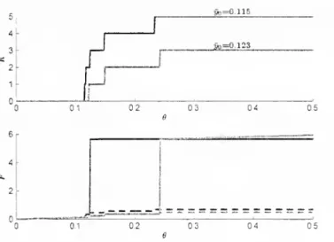
Discussion.

The

plots in Figure 5 are the equivalent to those in the free-information

case portrayed in Figure 4.

The

top panel plots the cascade size

K

as a function of

the losses in the originating

bank

8.

The

parameters

satisfy condition (19) so that the

cascadesize in this case isthe

same

as thecascadesize inthe free-information

benchmark

characterized in Proposition 1,

and both

figures coincide.

The

keydifferences areinthe

bottom

panel,

which

plotstheaggregate levelof liquidity

0.1

yv=0.115

' c: _0.3 04

C5

Figure 5:

The

costly-audit

equilibrium.

The

top panel plots the cacade size

K

as a function of the losses in the originating

bank

6 for different levels of the flexible reserves

yQ.

The bottom

panel plots aggregate level of liquidity hoarding

T

for the

same

set of

{y~o}-

The

dashed

lines in the

bottom

panel reproduce the free-information

benchmark

in

Figure 4 for comparison.

hoarding

J

7 _{as a function of}

6.

The

solid lines correspond to the costly audit equilibrium

characterized in Proposition 2, while the

dashed

lines reproduce the free-information

benchmark

also plotted in Figure 4.

These

plots

demonstrate

that, for low levelsof

K

(i.e.

for

K

<

3), theaggregate level ofliquidity hoarding with costly-auditingisthe

same

as the

free-information

benchmark,

in particular, it increases roughly continuously with 9.

As

K

switches

from

below

3 to

above

3, the liquidity hoarding in the costly audit equilibrium

make

a very large

and

discontinuous

jump.

That

is,

when

the losses

(measuring

the

severity of the initial shock) are

beyond

a threshold, the cascade size

becomes

so large

that

banks

are unable to tell

whether

they are connected to the distressed bank. All

uncertain

banks

act as if they are closer to the distressed

bank

than

they actually are,

hoarding

much

more

liquidity

than

in the free-information

benchmark

and

leading to a severe credit crunch episode. This is our

main

result.

Note

also that the aggregate level ofliquidity hoarding (and the severity of the credit

crunch) is not necessarily

monotonic

in the level of flexible _{reserves y} . For

example,

when

6

=

0.5, Figure 5

shows

that providing

more

flexibility to the

banks by

increasing

f/o actually increases the level of aggregate liquidity hoarding.

That

is, at low levels of 6,

an

increase in flexibility stabilizes the

system

but the opposite

may

take place

when

the shock is sufficiently large. Intuitively, if the increase in flexibility is not sufficient

to contain the financial panic (by reducing the cascade size to

manageable

levels),

more

flexibility backfires since it enables

banks

to

hoard

more

liquidity

and

therefore

exacerbate

the credit crunch.

4

The

Collapse

of

the

Financial

System

Until

now,

the uncertainty that arises

from

endogenous

complexity affects the extent of the credit crunch but not the

number

of

banks

that are insolvent,

K.

In this section

we

show

that if

banks have

"too

much"

flexibility, in the sense that condition (19)

no

longer

holds

and

Vo

e (yl

1

-

_y) (24)

(which also implies j3

=

y£), then the rise in uncertainty itselfcan increase the

number

of insolvent banks.

The

reason is that a large precautionary liquidity hoarding

compromises

banks' long

run profitability

by

giving

up

high return

R

for low return 1. In this context, even if the

worst

outcome

anticipated

by

a

bank

does not materialize, it

may

still

become

insolvent

if sufficiently close (but farther

than

K)

from

the distressed bank. In other words, a

bank's large precautionary reaction

improves

its liquidation

outcome

when

very close to

the distressed

bank

but it does so at the cost of raising its vulnerability

with

respect to

more

benign

scenarios. Since ex-post a large

number

of

banks

may

find themselves in the

latter situation, there

can

be a significant rise in the

number

of insolvencies as a result of

the additional flexibility.

The

analysis is very similar to that in the previous section. In particular, a

bank's

payment

still

depends on

its choice y'

_E

_{[0, yo]} at date

and

its forward neighbor's

payment

x

=

q{ ~ (p) at date 1.

That

is:

q p i l~k) (p)

=

Qi Wo,*}

and

Q2 (1~k) (p)

=

<?2 [vo,x]

for

some

functions q^ [y',x]

and

_q2[y',x].

However,

the characterization of the piecewise

functions _q\ [y',x]

and

qo [y'o,x] changes a little

when

condition (19) is not satisfied. In particular, these functions are identical to those in (26)

and

(27) in

Appendix

A.2 (as in

Section 3) but

now

there is

an

additional insolvency region:

y'

_>

_yu

[(/,

-x)z].

The

critical

new

element is the

bound

j/q [(^

—

x)z]. This is a function of the losses

from