HAL Id: inria-00349103
https://hal.inria.fr/inria-00349103
Submitted on 23 Dec 2008
HAL is a multi-disciplinary open access
archive for the deposit and dissemination of
sci-entific research documents, whether they are
pub-lished or not. The documents may come from
teaching and research institutions in France or
abroad, or from public or private research centers.
L’archive ouverte pluridisciplinaire HAL, est
destinée au dépôt et à la diffusion de documents
scientifiques de niveau recherche, publiés ou non,
émanant des établissements d’enseignement et de
recherche français ou étrangers, des laboratoires
publics ou privés.
Efficient Polyhedral Modeling from Silhouettes
Jean-Sébastien Franco, Edmond Boyer
To cite this version:
Jean-Sébastien Franco, Edmond Boyer. Efficient Polyhedral Modeling from Silhouettes. IEEE
Trans-actions on Pattern Analysis and Machine Intelligence, Institute of Electrical and Electronics Engineers,
2009, 31 (3), pp.414-427. �10.1109/TPAMI.2008.104�. �inria-00349103�
Efficient Polyhedral Modeling from Silhouettes
Jean-S´ebastien Franco, Edmond Boyer
Abstract— Modeling from silhouettes is a popular and useful
topic in computer vision. Many methods exist to compute the surface of the visual hull from silhouettes, but few address the problem of ensuring good topological properties of the surface, such as manifoldness. This article provides an efficient algorithm to compute such a surface in the form of a polyhedral mesh. It relies on a small number of geometric operations to compute a visual hull polyhedron in a single pass. Such simplicity enables the algorithm to combine the advantages of being fast, producing pixel-exact surfaces, and repeatably yield manifold and watertight polyhedra in general experimental conditions with real data, as verified with all datasets tested. The algorithm is fully described, its complexity analyzed and modeling results given.
Index Terms— Modeling from multiple views, modeling from
silhouettes, shape-from-silhouettes, 3D reconstruction, visual hull
I. INTRODUCTION
Modeling an object from silhouettes is a popular topic in computer vision. Solving this problem has a number of appli-cations for 3D photography, automatic modeling, virtual reality applications, among other possibilities.
Assume we are givenN silhouettes of an object corresponding to different camera viewpoints. The visual hull is the maximal solid shape consistent with the object silhouettes. It is often seen as the intersection of per-view volumes that backproject from the input silhouettes, the viewing cones, as will be further discussed. Such an approximation of the object captures all the geometric information available from the object silhouettes. Many methods exist to compute the visual hull of objects from silhouettes in images, as the problem is of interest for many applications including real-time 3D modeling, and provides an initialization for a wide range of more complex offline modeling methods [1]–[3]. In this article we describe how to efficiently use the silhouette information to compute polyhedral visual hulls, while achieving desirable properties for the surface representation and high modeling speed.
The visual hull definition was coined by Laurentini [4] in a theoretical context where an infinite number of viewpoints surrounding the object is considered. In this contribution, fun-damental properties of visual hulls are also analyzed. However, a geometric intuition and solution of the 3D modeling problem from a finite number of silhouettes was given as early as 1974 by B. Baumgart [5], based on pairwise polyhedral intersections of viewing cones.
The visual hull has been widely studied implicitly or explic-itly after this seminal contribution, in the computer vision and graphics communities. In particular, it was recently shown that the visual hull of a curved object is a topological polyhedron, with curved faces and edges, which can be recovered under M. Franco is with the University of Bordeaux, CNRS, INRIA Sud-Ouest, FRANCE.
M. Boyer is with the University Joseph Fourier, CNRS, INRIA Rhˆone-Alpes, France
weak calibration [6] using oriented epipolar geometry [7]. The algorithm proposed can however be impractical for fast and robust computations. We propose a simpler alternative to achieve these goals.
Many other algorithms exist to provide approximate solutions to the shape-from-silhouette problem. Most of them fall in two categories: volume-based approaches focus on the volume of the visual hull and usually rely on a discretization of space.
Surface-based approaches focus on a surface representation of
the visual hull. A third approach exists that computes a view dependent image-based representation, from an arbitrary view-point [8]. Although useful for a wide variety of tasks, this method doesn’t provide full 3D models as required by many applications. Obtaining full 3D models is a main concern of this article, which is why we focus mainly on surface-based approaches. To provide a wider view of the reconstruction problem, which can be solved using information different than silhouettes alone, we also discuss alternate methods of volume and surface reconstruction which use photoconsistency as a modeling cue.
A. Volume-based approaches
Volume-based approaches usually choose a discretization of space that uses convex cells called voxels. Each cell is projected in the original images and carved with respect to its silhouette consistency. This process relies on the convexity of cells to esti-mate whether a voxel falls inside or outside the input silhouettes, possibly sampling several points within a single voxel to perform the decision [9]. As such these approaches compute a discretized viewing cone intersection, as an approximate representation of the visual hull. The particular discretization chosen ranges from fixed grid representations with parallelepipedal axis-aligned cells [10], to adaptive, hierarchical decompositions of the scene volume [11]–[14]. Notably the choice of representation of the scene vol-ume as a set of voxel columns reduces the visual hull occupancy decision of an entire column to a line-to-silhouette-boundary intersection problem [15].
While robust and simple, this category of approaches suffers from inherent disadvantages. As they compute a discrete and approximate representation of the scene, the provided result is usually subject to aliasing artifacts. These can only be reduced by drastically raising the resolution of representations, yielding a poor trade-off between time complexity and precision. These representations are also biased by the coordinate system chosen for grid alignments. This is why more recent work has focused on alternate surface representations to capture more information about the visual hull. We have proposed a first improvement to volume-based approaches by means of a Delaunay tetrahedriza-tion of space, yielding a surface by carving away tetrahedra that fall out of the visual hull and a first step to eliminating axis-aligned bias [16]. We now discuss other works relevant to surface modeling from silhouettes.
B. Surface-based approaches
Surface-based approaches aim at computing an explicit repre-sentation of the visual hull’s surface, and analyze the geometric relationship between the silhouette boundaries in images, and the visual hull boundary. Surface primitives are computed based on this relationship and assumptions about the surface. Baumgart’s early method proposes an approach to compute polyhedral repre-sentations of objects from silhouette contours, approximated by polygons [5].
A number of approaches assume local smoothness of the reconstructed surface [17]–[21], and compute rim points based on a second-order approximation of the surface, from epipolar correspondences. These correspondences are usually obtained by matching and ordering contours from close viewpoints and can be used to connect points together to build a surface from the resulting local connectivities and orientations. This however only yields an approximate topology of the surface as these orientations reverse at frontier points, where rims cross over each other. More recent methods [22]–[25] exploit the duality that exists between points and planes in 3D space, and estimate the dual of the surface tangent planes as defined by silhouette contour points, but can still suffer from singularities due to improper handling of the local surface topology in the neighborhood of frontier points, or evacuate them by a costly resampling of the final surface which doesn’t guarantee proper surface rendition below a chosen threshold. Other primitives have been used to model the visual hull surface, computed in the form of surface patches [24], [26] or strips [27]. However, building a manifold surface representation from these primitives proves non-trivial and is not thoroughly addressed in those works. Additional difficulties arise in the particular case of visual hulls surfaces, which are computed as the boundary of a cone intersection volume, where viewing cones are tangent to each other. Thus, many surface components are sensitive to numerical instabilities in the region of these tangencies. Unless addressed, these issues usually mean that the surface produced will locally have anomalies, such as holes, duplicate primitives, and possibly self-intersections. While such methods with local errors are perfectly acceptable for rendering tasks, and have been used as such on graphics hardware [28], [29], surfaces produced without these guarantees are not suitable for 3D modeling applications. These often require post-processing of the surface, where manifoldness is a usual requirement. The surface is a2-manifold if the local surface topology around any point of the surface corresponds to a disk, thus ruling out cuts, self-intersections, and orientation reversals of the surface. This property is necessary for many post-processing tasks such as mesh simplification or smoothing, animation, compression, collision detection, volume computation, non-degenerate computation of normals, among other possibilities. A first response to degeneracy and epipolar matching problems was proposed for the case of smooth objects [6], [30], by identifying the precise structure of the piecewise smooth visual hull induced in this case.
C. Photoconsistency approaches
The aforementioned approaches are based on purely geometric decisions using silhouette regions and do not consider any pho-tometric information. Photohull approaches exist which compute sets of photoconsistent voxels as scene representation [31], [32], which has lead to many variations. Surveys of volume-based
photoconsistency approaches can be consulted for further details [33], [34]. It should be noted that although these methods use more scene information, they must also deal with the visibil-ity problem, because detecting photoconsistent voxels assumes knowledge of the subset of input images where that voxel is visible. As such, they are significantly more complex and sensitive to classifications errors, which propagate false information on the model for all voxels behind it. Such classification errors are bound to happen because many photohull methods compute photoconsistency under a Lambertian surface assumption for scene objects, a well known oversimplification of real world scenes. Recently, more successful methods using photometric information have been presented and address these problems using surface regularization schemes and surface topology constraints [2], [3]. Interestingly, most such methods achieve robustness by using a manifold visual hull surface representation to provide initialization and geometric constraints, which our algorithm can provide [3].
D. Difficulties and contributions
In this article we propose a new method for polyhedral model-ing of the visual hull of objects. Although several methods exist to compute visual hulls, and visual hull polyhedra or polyhedral strips [5], [27], from a set of silhouettes, several problems remain unaddressed.
First, we propose a more general definition of the visual hull which formulates the visual hull in the complement of the union of visibility domains of all cameras, as discussed in section II-C. The current formulations of visual reconstruction from silhouettes implicitly imply that all views see the entire object. Although this constraint can easily be fulfilled for small-scaled setups under controlled environments, it is much harder to achieve in wider-scale setups where the field of view of cameras and size of acquisition rooms is a limiting factor. Our definition enables to relax this constraint.
Second, it is unclear from existing work if polyhedral models of the visual hull are good approximations of the visual hull itself. We show here a scheme that consistently yields optimal poly-hedral visual hulls. Indeed we successfully apply an 8-connected segment retrieval algorithm [35] to recognize exact contours from image lattice coordinates lying at the boundary between the discrete silhouette and non-silhouette pixel regions. This in turn enables our algorithm to yield visual hull polyhedra that are pixel-exact with respect to input silhouettes, thereby providing a valid alternative to more expensive smooth reconstruction methods.
Third, most existing polyhedron-based reconstruction algo-rithms do not combine the advantages of being fast and repeatably yield watertight and manifold polyhedral surfaces. As a matter of fact, none of the surface-based reconstruction methods reviewed in section I-B make any strong mesh validity claim or thoroughly verify their outputs, with the exception of [36] (comparison given in section VIII). Baumgart’s contribution to polyhedral visual hull modeling [5] has given rise to an entire family of more general polyhedral solid modeling methods within the framework of Con-structive Solid Geometry (CSG) [37], where solids are expressed as a set of simpler solids combined using boolean operations. The intersection computations involved in building a boundary mesh from such general representations were proven unstable [38] in certain identified cases: because machine precision is finite, geometric decisions can be erroneous in degenerate or nearly
Fig. 1. The silhouette in its most general form: possibly several outer and inner contours, with counter-clockwise and clockwise orientation respectively. The inside region of the silhouette is grayed.
degenerate mesh configurations. The best attempt to solve this problem relies on exact, arbitrary-precision arithmetic [39], which remains the standard requirement for failproof computational geometry modeling methods to this date, as implemented in state-of-the-art libraries such as CGAL [40]. While this theoretically closes the problem, the enormous overhead of exact arithmetic CSG hardly makes it a practical solution for visual hull modeling, one of its major appeals being the potential to produce models at very efficient speeds. Instead, our solution focuses on identifying the structure of polyhedral visual hulls (section III) to yield a very simple algorithm with an identified computational complexity (section VII). In our case, geometric computations reduce to a very small set of single-unknown intersection cases (examined in sections V and VI) which can easily be fine-tuned to minimize the possibility of numerical error. Indeed our implementation has provided watertight and manifold polyhedral surfaces on all real datasets tested with no single failure, as verified in section VIII and independently [36].
II. VISUALHULLDEFINITIONS
Let us consider a scene with several objects of interest, ob-served byN pinhole cameras with known calibration. A vertex in space will be writtenX(capitals). Image points will be written xorp, and an image line l. Image view numbers will be noted as superscripts. We sometimes associate to a pointxin viewiits
viewing lineLixdefined as the set of points that project to x in
imagei. Details about multi-view geometry can be found in the literature [41], [42].
A. Contours and rims
We assume that the surface of observed scene objects is closed and orientable, curved or polyhedral, possibly of non-zero genus.
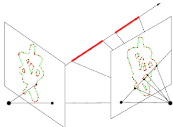
Rims (see Fig. 3(a)) are defined as the locus of points on the
surface of objects where viewing lines are strictly tangent to the surface. The projection of rims in images define the occluding
contours [10], which bound the silhouette of objects in each
image plane. With this definition, each occluding contour has the topology of a one-dimensional manifold.
Observed silhouettes can be of non-zero genus: each silhouette can consist of several different connected components, arising from the projection of different scene objects. Each connected component can comprise several holes reflecting the topology of these objects, giving rise to inside contours of the silhouette (see Fig. 1). To denote the different occluding contours observed under these conditions in each view, we use a subscript:Cjinames thejth
occluding contour in viewi. We call inside region of an occluding contour the closed region of the image plane which it bounds.
Symmetrically we call outside region its complement in the image plane. Outside and inside contours of the silhouette are to be distinguished by their orientation, respectively counter-clockwise and clockwise. This is a useful definition as it ensures that the actual inside region of the contour is locally left of any portion of an occluding contour, regardless of its nature. Each viewithus has a set of contoursCi, which in fact is the union of two sets of inner contoursNi and outer contoursOi.
B. Viewing cone
The viewing cone is an important notion to define visual hulls as it describes the contribution volume associated with a single view. Because silhouettes can have several disconnected compo-nents and holes, it is necessary to distinguish two definitions. We first introduce the viewing cone associated with a single occluding contour, before discussing the more general definition of a viewing cone associated with a viewpoint, which is the one generally used throughout this article.
Intuitively, the viewing cone associated with an occluding
con-tour is a cone whose apex is the optical center of the associated
view, and whose base is the inside region of this contour. More formally, the viewing cone Vji associated with the occluding
contourCji is the closure of the set of rays passing through points
insideCij and through the camera center of image i. Vji is thus
a volume tangent to the corresponding object surface along a curve, the rim (or occluding contour generator) that projects onto Cji. According to the nature ofCij, which is either an outside or
inside contour, the viewing cone is a projective volume whose base in images is a region ofR2, respectively closed or open.
Based on these conventions, we can now give a definition of the viewing coneVi associated with a view i. Such a definition
should capture all points of space that project on the inside region of the viewi’s silhouette. A first intuitive definition ofVi could be formulated by compounding the contributions of the connected components of the silhouette:
Vi= [ k∈Ki ( \ j∈Ci k Vji), (1)
whereKi is the set of connected components of the silhouette in viewi andCi
k the set of contours associated with thek-th
con-nected component in the silhouette, namely one outside contour and an arbitrary number of inside contours in that component. This formulation however assumes that occluding contours can easily be grouped by connected component once acquired from an input set, which is not straightforward. We thus use an equivalent definition ofVi, which separates cones in two sets according to the orientation of the corresponding contour:
Vi= ( [ j∈Oi Vji) \ ( \ j∈Ni Vji). (2)
The equivalence with (1) comes from the fact that inner contours have a neutral contribution for all set operations outside their corresponding outer contour. Thus they can be used independently of outer contours to compute the visual hull volume. This is also practical because the orientation of the contours can be detected independently when discovered in input images, which is why this definition is the one generally used to compute viewing cone primitives.
1 2 3 4 1 2 3 4 1 2 3 4 (a) (b) (c)
Fig. 2. A scene observed by 4 viewpoints: consequence of the different possible visual hull definitions. (b) and (c) show, in gray, regions as defined by (3) and (4) respectively.
C. Visual Hull Set Definitions
In previous work on visual hulls, it is always assumed, to the best of our knowledge, that all views see the object in its entirety. However, the problem of building such visual hulls from non-overlapping views has never been addressed. We therefore provide a different definition of the visual hull to enable the possibility of modeling in this case, by reasoning over the set of points of R3 that lie at the union of all visibility regions. All algorithms to reconstruct the visual hull, including the one we present in this article, can use either of these definitions, depending on the context and targeted application.
Informally, the visual hull can be defined as the intersection of all viewing cones associated with the considered viewpoints. It therefore consists in a closed region of space, whose points project on the inside region of all occluding contours. LetI be the set of input images considered, andC the set of all occluding contours. The visual hull can be directly formulated using the above definition of a viewi’s viewing cone:
VH(I, C ) = \
i∈I
Vi. (3)
However, expression (3) has the undesirable side-effect of elim-inating regions outside the visibility region of certain cameras, as illustrated in Fig. 2-(b). This is nevertheless the definition implicitly used in most existing algorithms. A solution to this problem is to consider each view’s contribution only in this view’s visibility region Di. This can be achieved by expressing the complement of the visual hull, as an open region ofR3 defined by: VHc(I, C ) = [ i∈I “ Di\ Vi”, = [ i∈I 2 4( \ j∈Oi Di\ Vji ) [ ( [ j∈Ni Di\ Vji) 3 5 (4)
where Di\ V is the complement of a given set V in view i’s visibility domain. By using (4), objects that do not appear in all images can still contribute to the visual hull. Knowledge about the visual hull or its complement is equivalent because the surface of interest of the visual hull delimits these two regions.
The use of these different definitions is illustrated in Fig. 2. A scene is observed from four viewpoints, where camera 1 only sees the green object. Use of expression (3) is illustrated in Fig. (b) : the visual hull (in gray) does not contain any contributions relative to the red and blue objects. Fig. (c) shows
the result of expression (4), which does include such contributions using the complement of the visibility domain. Note that the use of (3) and (4) both can induce virtual objects not present in the original scene, but (4) produces more in general. Such ”ghost” objects appear in regions of space which project inside silhouette regions of real objects in all views. The number and size of such artifacts can be reduced by increasing the number of viewpoints.
III. THEVISUALHULLSURFACE
We have given a set definition of the visual hull volume. We are particularly interested in the visual hull’s surface, which bounds this volume. In order to derive the algorithm, we study the properties of this surface, in particular under the assumption of polygonal occluding contours, which leads to a polyhedral form for the visual hull.
A. Smooth Visual Hulls
The visual hull surface’s structure has previously been studied in the case of a finite number of viewpoints, with the underlying assumption of contour smoothness and perfect calibration [6]. This work shows that the visual hull of smooth objects with smooth occluding contours is a topological polyhedron with generalized edges and faces, corresponding to truncated portions of smooth viewing cone surfaces and surface intersections. This shape bares the contributions of one view (strips), two views (cone intersection curves and frontier points), and three views (triple points), as depicted in Fig. 3(a). An algorithm to reconstruct this polyhedron was proposed in the original work, and a thoroughly described variant of greater efficiency was recently proposed [36]. Both works rely on the explicit detection and construction of frontier points, which is a delicate step because frontier points arise at the exact locus of tangency of two viewing cones. How-ever in general setups, contour extraction and calibration noise, as well as finite precision representation of primitives, imply that the viewing cones manipulated in practice only approximate true viewing cones. Therefore they never exactly exhibit the tangency property. This leads the aforementioned approaches [6], [36] to tediously search and build an approximate representation of frontier points based on contour smoothness assumptions.
B. The Validity of Polyhedral Approximations
Because the shape of the visual hull is stable under small per-turbations, using bounded polygonal approximations of occluding contours will have little impact on the global shape computed. To this aim we propose to discretize occluding contours using an efficient, pixel-exact extraction algorithm (e.g. [35]), which does not increase the overall noise introduced by silhouette extraction. Fig. 3 and Fig. 4 make explicit the particularities in structure that are induced by calibration and discretization noise. Tangency is generally lost and the structure is consequently altered, from a set of perfectly interleaved strips crossing at frontier points (Fig. 4(a)), to a disymmetric structure where strips overlap one another and where strip continuity is lost (Fig. 3(b), Fig. 4(b)). Interestingly, this structure is thus more general than the theoretical smooth structure of the visual hull because of the absence of purely degenerate primitives, and leads to the simpler algorithm proposed.
(a) (b)
Fig. 3. Differences in structure in the visual hull (here a sphere obtained from three views under a perfectly calibrated and smooth occluding contour setup [6] (a), versus the case of discretized occluding contours and less than perfect calibration, leading to a polyhedral visual hull without frontier points (b).
(a) (b)
Fig. 4. Schematic visual hull strips obtained (a) in an ideal case where noise is absent (b) in the presence of noise.
C. Relevant Primitives of the Polyhedral Visual Hull
We describe here the useful polyhedron primitives induced by contour discretization, shown in Fig. 3(b). We will use these to build our algorithm.
Infinite cone face. An infinite cone face is a face of a discrete viewing coneVi, induced by contour discretization. Each 2D edge
eof a discrete silhouette contour induces an infinite cone faceTe.
A discrete strip is a subset of the surface of a discrete viewing cone. Each strip is fragmented as a set of faces each induced by a 2D edge e. The faces are thus a subset of the corresponding infinite cone faceTe.
Viewing edges are the edges of the visual hull induced by viewing lines of contour vertices. They form a discrete set of intervals along those viewing lines, and represent part of the discrete strip geometry as they separate the different faces of a same strip. Such edges can be computed efficiently, as described in section V, and give the starting point of the proposed surface modeling algorithm.
Triple points, the locus of intersection of three viewing cones, are still part of the cone intersection geometry, because they are non-degenerate and stable under small perturbations.
Cone intersection edges form the piecewise linear cone intersection curves induced by viewing cone discretization.
A number of mesh primitives arise from (and project back on) each occluding contour 2D edge e. We call edge e a generator for these primitives. In a non-degenerate configuration, faces possess one generator, edges possess two generators, and vertices three: all vertices of the polyhedron are trivalent. We assume that degenerate configurations are extremely unlikely to occur with practical noisy inputs and finite number representations, an assumption experimentally verified for all datasets tested to date (section VIII). Instead, small but consistent edges and faces are computed on the polyhedron in nearly degenerate configurations. The structural elements of the polyhedral visual hull now identified, we now discuss the algorithm proposed to build them efficiently.
IV. ALGORITHMOVERVIEW
Several of the properties analyzed about visual hull polyhedra and viewing edges hint toward a simple and efficient algorithm. First, the polyhedral mesh of the visual hull is the union of viewing edges, which are easy to compute, and cone intersection edges. Vertices of the polyhedron are either viewing edge vertices or triple points. Second, coplanar primitives of the polyhedron project on the same occluding contour edge: they share a com-mon generator e. More generally incidence relationships on the polyhedron only occur between primitives that share a common subset of generators. Third, computing the extremal vertices of an edge on the polyhedron through intersection operations hints to the incidences of neighboring edges not yet computed, because we know which generators these primitives share. We thus propose to incrementally recover the entire polyhedron in a three step process (Figure 5):
Fig. 5. Algorithm overview.
1) Compute all viewing edges of the polyhedron, their vertices, and their generators.
2) Incrementally recover all cone intersection edges and triple points, using the common generators of adjacent primitives already computed.
3) Identify and tessellate faces of the polyhedron. The following sections give the details of each step.
V. COMPUTINGVIEWINGEDGES
We here examine the first step of the proposed algorithm. Viewing edge computation has indirectly been studied by Matusik
et al. [8] to compute image-based representations of the visual
hull, where an equivalent process needs to be applied to each ray of a target image. Cheung et al. [43] also use similar computations to constrain the alignment of visual hulls across time. The algorithm we use is as follows.
A. Algorithm
Computing viewing edges consists in searching the contribution to the visual hull surface of each vertexpused in the 2D occluding contour polygons. It is thereby necessary to determine when such a viewing line traverses the viewing cones of all other views. For each cone this defines a set of intervals along the viewing line of p, representing the portions inside the cone. These sets must then be gathered across all views and combined using one of the set formulations described in section II-C, in order to obtain edges of the final polyhedron.
The algorithm is summarized below. The viewing line of vertex pij is notedLij.
Algorithm 1 Viewing Edge Computation 1: for all contour Oij in all views: do
2: for all view ksuch thatk6= i: do 3: for all verticespij inOji : do
4: compute the epipolar linelofpij in viewk, 5: compute intervals of l falling inside contour Okl in
viewk,
6: combine depth intervals alongLi
j with the existing
7: end for
8: compute the 3D points bounding the intervals alongLij.
9: end for 10: end for
B. Computing depth intervals
Let pij be the vertex of an occluding contour Cji. The
con-tribution intervals on the viewing line of pij are bounded by intersections of this viewing line with surfaces of viewing cones
Fig. 6. Intervals along the viewing ray contributing to the visual hull surface(red).
T Tleft
right
Fig. 7. Orientation relationship between strips, occluding contours and viewing edges, for algorithm initialization.
in viewsk 6= i. They can be computed in 3D or using epipolar geometry (Fig. 6).
Once depth intervals have been obtained for each viewing cone of views k 6= i, they must be combined according to the set definitions of the visual hull described in section II-C, by using either definition (3) or (4) and applying it to the intervals.
VI. COMPUTING CONE INTERSECTION EDGES A. Initialization
The main characteristic of the algorithm is to build the mesh while visiting it. New vertices are incrementally added by identifying missing edges of existing vertices. Viewing edges serve as the starting point for the algorithm: they are a discrete representation of the strip geometry. They provide two initial vertices that share one known edge. For each of the vertices, two edges are missing and need to be built.
Fig. 7 shows how to initialize the mesh traversal by using contour orientation in views. The viewing edge provides two initial paths for mesh building, whether traversal is started toward the camera or away from the camera. When initializing the traversals it is easy to identify what generators are locally left and right, because the strip is oriented.
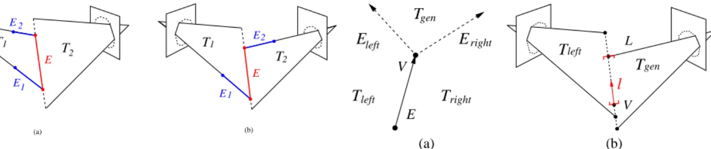
B. Two-view case
The two view case is an interesting particular configuration, because there are no triple points by definition. Viewing edge ver-tices completely capture the cone intersection geometry because
E1 E2 E T1 T 2 E (a) (b) T T E 1 2 E1 2
Fig. 8. The two types of cone intersection edge, in the two view case. Both configurations involve connecting neighboring viewing edge vertices that share the edge E.
they already embed all possible line-to-plane intersections arising between cones. In this case, cone intersection edges are very simple to find, because they fill gaps between already existing vertices. Only two configurations exist for a cone intersection edge E, whether the vertices of the edge arise from viewing lines of different or identical views, as illustrated in figure 8. Since the generators of viewing edge vertices are known when they are computed, these can be stored and used to identify cone intersection edges. Such edges can be retrieved simply by identifying those viewing edge vertices whose generators are consistent with either of the two possible patterns in the figure. This can be done by looking at each viewing edge vertex and examining candidates for the second vertex of edge E on the four neighboring viewing lines involved, as seen in the figure.
C. GeneralN-view case
Recovering cone intersection edges in the general case is not as simple. Triple points appear on the cone intersection portions of the visual hull, and cone intersection edges no longer directly connect viewing edges but form locally connected sub-mesh structures around sets of triples points, as shown in Fig. 3(b). These sub-mesh structures arise from the constraint that such edges always lie on two viewing cone faces, arising from two different views, in order to be on the surface of the visual hull, as described in section III-C.
The two-view algorithm needs to be extended to recover these sub-meshes. The proposed algorithm is summarized in paragraph VI-E. At any given point in the algorithm, a sub-part of the mesh is known but has partially computed hanging edges. The set of hanging edges is initialized to the set of viewing edges, but gradually becomes incremented with cone intersection edges. Regardless of the nature of the hanging edge and the stage of advance in the reconstruction, hanging edges always exhibit the same local problem, illustrated in Fig. 9(a). The problem is that two edges are missing and need to be identified, one left of the current hanging edge E, the other on its right. Both missing edges share a common vertexV with the hanging edgeE. What enables the algorithm to make incremental progress in the mesh building is that all three generators ofVare known. They are noted Tlef t,Trightand Tgen in the figure. Consequently we know the
generators of both missing edges Elef t and Eright, because of
consistent orientation propagation from edge to edge.
1) Missing edge direction: We therefore can use this
informa-tion to compute a first geometrical attribute of the missing edges, their direction. We label these oriented vectors respectivelyllef t
andlright. left
T
T
gen ET
VE
leftE
right right gen Vl
left LT
T
(a) (b)Fig. 9. (a) Characteristics of a hanging edge. (b) Retrieval of the maximal possible edge Emax
Because the normals of the planar cone faces corresponding to a given generator are known, computingllef t andlrightis easy.
Ifnlef t,nrightand ngen are the normals associated withTlef t,
Trightand Tgen, and the traversal direction vector of the current
edge is labeledlE and points toward V, they are given by the
following expressions:
llef t = k nlef t× ngen such that |lE llef t nlef t| > 0
lright = k ngen× nright such that |lrightlEngen| > 0
where the coefficientk∈ {−1, 1}ensures a consistent orientation in each case.
The information still missing about edges Elef t and Eright
is the particular vertex instance theses edges lead to. Such vertices can only be of two natures : either an existing viewing edge vertex or triple point. Let us focus on the case of missing edge Elef t. The case of Eright is exactly symmetric and can
be inferred by the reader from the following description, by considering the generators of Eright, namely Tgen and Tright.
We will first consider the maximal possible edge, which is given by two-view constraints over Elef t. We will then discuss the
existence and retrieval of a triple point vertex for Elef t, then
focus on retrieving a viewing edge candidate, should no triple point exist for this edge.
2) Maximal possible edge: The cone intersection edgeElef t
is known to be on the surface of the visual hull. It is partially defined by two generatorsTlef tandTgen, arising from two views
i and j. Because the two generators are limited in space, they introduce a constraint over where any candidate edge can be. The maximal bound for an edge is represented in Fig. 9(b). It is given by the most restrictive of the four viewing lines involved, in the directionllef t. The maximal possible edge is labeledEmax.
3) Triple point case: Any candidate vertex chosen within
Emax is valid if and only if connecting it toV ensures that the
entire resulting edge lies within the volume of all viewing cones for views other than i and j, by definition of the visual hull. Should this constraint be violated, we would no longer be able to guarantee that the mesh geometry we are computing lies at the surface of the visual hull polyhedron. Reciprocally, if we do detect a view k for which this constraint is violated, then we have detected a triple point. There can be several such views for which the constraint is violated. To ensure we stay on the visual hull, we must select the viewk that leads to the shortest possible created edge. This is done by projectingEmax into all
viewsm 6= i, j, identifying the generator edge giving the most restrictive intersection bound with the silhouette contour of each view m, and keeping the most restrictive intersection bound
among all views, if any such intersection exists. It thus enables us to compute both the existence and geometry of a triple point, from its third identified generator in a viewk.
4) Viewing edge vertex case: Should no intersection restrict
Emax from its original upper bound, we know Elef t does not
connectVto a triple point, but to an existing viewing edge vertex instead. As in the two view case, there are only a restricted number of possible viewing edge vertex candidates Elef t can
lead to. These lie on the four viewing lines incident to the planar cone faces of Tlef t and Tgen, arising from two different views
i and j. Exactly like in the two view case, it is then possible to retrieve the corresponding viewing edge vertex VE from one
of these viewing lines, by examining the generators it has in common withElef t.
5) Iteration and stopping conditions: Once the missing vertex
ofElef thas been identified and built, the resulting edge is added
to the list of current hanging edges. The missing edge Eright
can then be built and also added to the list of hanging edges. Processing then continues by retrieving any hanging edge from the current list, and in turn by building its missing edges, until the list is empty. Alternatively, the algorithm can also be made recursive and use the stack for hanging edge storage, instead of a list. Traversals stop when a missing edge is built by connecting the current vertex to a vertex that has already been created. The condition is trivial when no triple point is found, because viewing edge vertices already exist by construction. If a triple point is found, the algorithm must be able to determine if it has been created or not. This can be achieved by indexing triple points using the triplet of its generators as key, all of which are known as soon as a triple point is detected.
D. Polyhedron face identification
Once all edges have been retrieved, a full traversal of the edge structure can be used to determine the faces of the polyhedron. Each generator edge in the 2D images contributes to a face of the polyhedron in form of a general polygon, with possibly several inside and outside contours. These contours can be identified by starting at an arbitrary vertex of the face, and by traversing the mesh, taking face-consistent turns at each vertex until a closed contour is identified. Because the mesh orientation is consistent, this yields counter-clockwise oriented outer contours, and clockwise oriented inner contours. This information can optionally be used to tessellate faces to triangles, with standard libraries such as GLU [44].
E. Algorithm summary
The algorithm is summarized here in recursive form. Two functions are used to process hanging edges (Algorithm 2), retrieve edges (Algorithm 3) and retrieve vertex (Algorithm 4). Through this summary, and the summary of the viewing edge algorithm, it can be noted that the entire visual hull computation reduces mainly to one numerical operation: the ordering of 3D plane intersections along a 3D line’s direction.
Algorithm 2 Polyhedral visual hull computation 1: compute viewing edges
2: for all vertexV of viewing edgeE: do 3: retrieve edges(V,E)
4: end for
5: for all generatorT of all silhouette contours: do 6: retrieve face information, all contoursC in plane ofT 7: end for
Algorithm 3 retrieve edges(V,E)
1: if edge left ofE missing at vertexV then 2: compute directionllef t of missing edge
3: retrieve vertex(V, llef t)
4: end if
5: if edge right ofEmissing at vertex V then 6: compute directionlrightof missing edge
7: retrieve vertex(V, lright)
8: end if
Algorithm 4 retrieve vertex(V,l)
1: compute maximal edgeEmax in search directionl
2: find viewksuch thatconek intersectsEmaxclosest toV
3: ifk exists then
4: search triple point P = Emax∩ conek in triple point
database
5: ifP was not yet created then
6: compute triple pointP = Emax∩ conek
7: addP to mesh and triple point database 8: end if
9: add new edgeE=[V,P] to mesh 10: retrieve edges(P, E)
11: else
12: find viewing edge vertexS incident toEmax
13: add new edge [V,S] to mesh 14: end if
VII. COMPLEXITY ANALYSIS
Let n be the number of views, m the number of objects in the scene, andq the maximum number of vertices in occluding contours of any view. The number of operations of visual hull algorithms is non trivial to evaluate with respect to the order of magnitude of input sizes. This is because the topology of scene objects themselves has an influence on the number of primitives generated and computation time. In particular there can be multiple viewing edges along a single viewing line, as soon as silhouettes of objects exhibit their non-convex, self-occluding parts.
We therefore simplify this study by considering scenes withm convex objects. The non linear behavior of the algorithm is then limited to inter-object phenomena, because silhouettes of convex objects are also convex and can therefore not generate multiple viewing edges. This study generalizes to arbitrary scenes simply, by consideringmto be the minimal number of components in a convex part decomposition of the scene geometry.
A. Number of computed vertices
The viewing edge and cone edge retrieval algorithms both compute O(nm2
q) 3D vertices. Each reconstructed visual hull component is convex and therefore exhibitsO(n)strips, with each
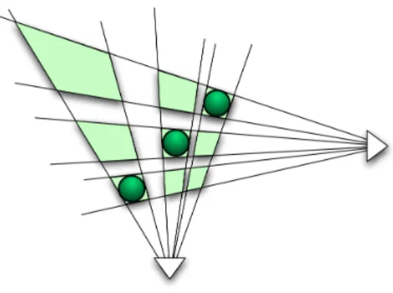
Fig. 10. Quadratic behavior: illustration in the case of three real objects, leading to 9 visual hull components.
strip being made ofO(q)primitives directly inherited from image contour geometry. In the worst case where views are ambiguously placed, the silhouettes of m objects can be generated by a quadratic number of components, all of which are accounted for in the visual hull (see Figure 10). The likelihood of encountering this worst case decreases with the number of views used. Nevertheless some particular object and camera configurations have been seen to result in this behavior in practical, near-degenerate setups, when four views are at the four corners of a rectangle for example.
B. Number of operations
The number of operations required for computing viewing edges isO(n2mqlog mq), decomposing as follows: for each of theO(nmq)viewing lines considered, an intersection is searched in each of the other n− 1 images, using an O(log mq) search to identify an intersecting edge among the mq edges of the searched image. Such a logarithmic search can be achieved by pre-ordering vertices of a silhouette around all possible epipoles, using 2D angles, or epipolar line slopes [8]. Both schemes exhibit discontinuities that must be dealt with carefully.
Computing cone intersection edges is aO(n2m2qlog mq) op-eration. Because each of theO(nm2q)edges requires examining edges in all views other than those of its generators, a naive implementation examining all of the O(nmq) edges in other views would result in an O(n2m3q2) operation. Similarly to the viewing edge case however, a sorted datastructure can be precomputed to achieve view searches, reducing the per-vertex cost to O(n log mq). Our implementation uses a single data structure to accelerate viewing edge and viewing cone edge computations for the purpose of efficiency. Instead of using a structure whose sorting depends on epipole positions, we compute sorted silhouette vertex lists for a fixed numberkof directions in the 2D plane, which in turn can be amortized for both algorithms. Each algorithm can then use the direction amongkwhose sorted list minimizes the number of searched edge candidates for a given search operation. The choice ofkcan be fine-tuned in pre-computed tables according to n, m and q. Although we do not have access tomin practice, a sufficient approximation of mis to consider the average number of occluding contours per view over all views.
Identifying faces is trivially an O(nm2
q) operation, because it is linear in the number of vertices of the final polyhedron. The polyhedral visual hull recovery algorithm therefore yields
an overall cost of O(n2m2qlog mq) operations. To the best of our knowledge, no existing polyhedral visual hull method gives an estimate of this complexity, except [27]. An estimate of this complexity is given in a related technical report [45], section 3.6. Transposed withm convex objects in the scene, the given time complexity is dominated by O(n2m2qlog nmq), slightly worse than our algorithm, and with weaker guarantees for surface properties.
VIII. RESULTS
The algorithms presented in this article have been implemented and validated with several variants, one of which has been made publicly available from 2003 to 2006 as a library called EPVH1 (reference implementation, version 1.1). A distributed implementation has also been produced as part of the collaborative effort to build the GrImage experimental platform at the INRIA Rhˆone-Alpes. Both synthetic and real data have been used to validate the algorithm and its reference implementation. We first present synthetic datasets showing the validity of the algorithm in extreme cases, and correctness of generated polyhedral surfaces on a broad set of examples. We then provide results obtained from large real sequences acquired on the GrImage platform, and illustrate the potential of the method for 3D photography and videography. Finally we compare the algorithm with the method by Lazebnik, Furukawa & and Ponce [36], a state of the art approach.
A. Method validation and reliability
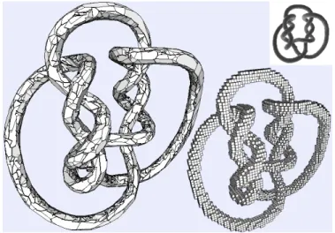
Synthetic datasets have been used to characterize the global behavior of the algorithm in the absence of segmentation noise, and check its sanity in reconstructing objects whose topologies are actually more complex than those of real world objects. The most relevant example we use is the “knots” object of figure 11, reconstructed from42viewpoints, illustrating the capability of the algorithm to accurately reproduce such objects and topologies from silhouette data. Comparison with classical volume-based approaches highlight the impossibility to reproduce the object as precisely as the polyhedral models even if a very high resolution is used.
We have extensively used synthetic and real datasets to verify the manifold and watertight nature of the surfaces produced by our algorithm. The potential sensitivity of the algorithm, as in all algorithms strongly relying on geometric boolean operations, lies in the potential for misrepresentation of intersection coordinates in the neighborhood of a degeneracy: coincidence of four or more planes at a same point, perfect plane collinearity. However, degeneracies and their perfect representation within the range of floating point numbers proves extremely unlikely in practice. In fact, the naive double-precision ordering of plane-intersections along a direction we use, proves non-ambiguous in all experi-mented cases.
For a thorough verification, we have compiled a test database of 44synthetic objects, each reconstructed with a number of views ranging from3to42, which cover the main expected conditions for running the algorithm. The viewpoints are chosen at vertex locations of an icosahedral sphere, which is worse than real-life conditions because choosing regular viewpoints with noise-free coordinates greatly increases the probability of computing
Fig. 11. Visual Hull of the “knots” object obtained using our algorithm from
42viewpoints, uses 19528 vertices. Right: the same data reconstructed using
a voxel method resolution of 643= 262144shows the inherent limitations
of axis aligned voxel methods. Top right: original model, from Hoppe’s web site [46].
coincidentally degenerate intersections. Silhouette bitmaps are vectorized, and the coordinates of the vectorization dilated by a random, subpixel factor, to keep this probability close to zero. The completeness and manifoldness of the representation is verified internally by checking (1) that each edge is incident to exactly two faces, and (2) that each vertex’s connected surface neighborhood is homeomorphic to a circle [47], namely by checking that each vertex is connected to three faces and edges verifying (1). Watertightness is also internally verified by checking that each edge is traversed exactly two times upon building the polyhedron faces in the third step. By construction all polyhedra generated are orientable because of consistent orientation propagation from images (algorithm 3). We also verify these properties externally by loading all output models in CGAL and testing for polyhedron validity and closedness: all such tests have returned results consistent with the internal verification.
Examples of objects and reconstructions are given in Fig. 12. Results collected about the reconstructions on our dataset show that all 1760 reconstructions succeed in producing a closed manifold mesh. The manifold property of the generated surfaces and broad success of the algorithm have also been independently verified on other datasets by Lazebnik et al. [36].
B. Real Datasets and 3D Videography
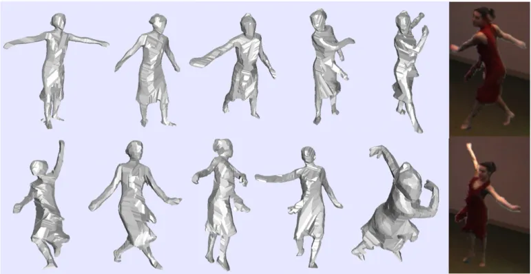
We conducted many experiments with real video streams acquired on the GrImage platform. We here present an example sequence, among many others acquired throughout the life of the acquisition platform, the DANCEsequence. This dataset was produced using19synchronized30Hz cameras, whose acquisition was processed on a dedicated PC grid. Surface precision and movement details are captured with high quality by the recon-structions, as illustrated in Fig. 13. All800models generated in this27second sequence were verified to be manifold, watertight polyhedral surfaces. The average computation time is0.7seconds per sequence time step, as processed by a 3GHz PC with 3Gb Ram. The model quality is suitable for 3D photography, by applying a texture to the resulting model, here computed by blending contributions of the three viewpoints most front-facing
Fig. 12. A few of the 44 synthetic models reconstructed using the proposed algorithm, here presented as modeled from 42 views. 1760 reconstructions were performed using from 3 to 42 views.
the corresponding texture face. Realistic models obtained are depicted in Fig. 13.
C. Comparison with state of the art methods
Many shape-from-silhouette algorithms exist, yet little can produce outputs comparable to those of the proposed approach. The very recent approach by Lazebnik, Furukawa & Ponce [36], built upon earlier work [6], proposes an algorithm relying on smooth apparent contours and explicit detection and recon-struction of approximate frontier points, to recover the smooth projective structure of the visual hull. In this approach, the authors propose to use a dense discretization of apparent contours in image space and rely on discrete approximations of contour curvatures to build the topological polyhedron of the visual hull illustrated in Fig. 3(a). The resulting algorithm can be used to perform incremental refinements of the visual hull by adding a viewpoint at a time, and explicitly uses oriented epipolar geometry to compute image-to-surface relationships and primitives. The algorithm produces a projective mesh and a finescale polyhedron by triangulation of visual hull strips. A qualitative and quantitative performance assessment has been jointly performed (see also [36], section 6.3), using datasets kindly made public by Lazebnik et al. Five objects were photographed from28viewpoints, yielding high resolution images. For the need of the Lazebnik et al. algorithm, apparent contours were manually extracted from images, and very densely discretized to favor frontier point detection. Comparisons are given for the sub-pixel contour dataset in Table I for both algorithms and depicted in Fig. 14.
Importantly, such a dense sub-pixel discretization is not needed but can still be dealt with by our algorithm. It is also not necessary for most applications. To illustrate this, we also provide results, labeled “EPVH from images”, produced using the original
silhou-Fig. 13. Polyhedra produced by EPVH for the DANCEsequence, from 19 views. Sequence acquired from GrImage, INRIA Rhˆone-Alpes. Input contour sizes were of the order of 210, yielding models with approximately 5, 400 vertices, 8, 100 edges and 10, 800 triangles. (right) Model is textured by choosing the most front-facing viewpoint, and inserted in a virtual scene.
ette bitmaps at image resolution, and applying pixel-exact contour discretization [35], the standard EPVH pipeline. This processing of the datasets still captures all the information present in the original silhouettes but yields apparent contour discretizations and visual hull polyhedra orders of magnitude less complex, which can be computed in a few seconds.
When compared on identical sub-pixel piecewise-linear contour inputs, both our algorithm and Lazebnik et al. produce manifold polyhedra that are visually indistinguishable (see Fig. 15). Our algorithm however does show a clear performance advantage in all datasets. No complexity analysis was given by Lazebnik et
al., although the provided time results do hint toward a similar
complexity, related by a constant. Yet our algorithm shows an inherent advantage in producing polyhedra with a significantly lower number of primitives, which certainly participates in the performance gain. This characteristic can probably be attributed to the fact that EPVH produces polyhedra which closely and directly relate to contour inputs, and generates no intermediate primitives other than ones already on the visual hull surface, by construction.
IX. CONCLUSION
We have proposed an analysis of visual hull based object modeling, yielding a new algorithm to build the visual hull of an object in the form of a manifold, watertight polyhedral surface. We propose an alternative set definition of the visual hull that relaxes the need for a common visibility region of space implied by classical definitions. We then carry further the analysis and precisely determine the discrete structure of the visual hull surface in the case where polygonal silhouettes are used as input. This leads to a new algorithm that separates the estimation of
a visual hull polyhedron into the determination of its discrete strip geometry, followed by the recovery of cone intersection edges. These primitives are determined to be complementary in the representation of visual hull polyhedra. The complexity of the algorithm is analyzed, and results are provided for a variety of synthetic and real datasets. This work provides several key contributions to 3D modeling from silhouettes, which are exper-imentally put to the test. First, watertight, manifold polyhedral surfaces are verifiably produced. Second, such polyhedra are produced more efficiently than current state of the art methods.
REFERENCES
[1] J. Isidoro and S. Sclaroff, “Stochastic refinement of the visual hull to sat-isfy photometric and silhouette consistency constraints.” in Proceedings
of the 9th International Conference on Computer Vision, Nice, (France),
2003, pp. 1335–1342.
[2] Y. Furukawa and J. Ponce, “Carved visual hulls for image-based mod-eling,” in European Conference on Computer Vision, 2006.
[3] S. N. Sinha and M. Pollefeys, “Multi-view reconstruction using photo-consistency and exact silhouette constraints: A maximum-flow formula-tion,” in Proceedings of the 10th International Conference on Computer
Vision, Beijing, (China), oct 2005.
[4] A. Laurentini, “The Visual Hull Concept for Silhouette-Based Image Understanding,” IEEE Transactions on PAMI, vol. 16, no. 2, pp. 150– 162, Feb. 1994.
[5] B. G. Baumgart, “Geometric modeling for computer vision,” Ph.D. dissertation, CS Dept, Stanford U., Oct. 1974, aIM-249, STAN-CS-74-463.
[6] S. Lazebnik, E. Boyer, and J. Ponce, “On Computing Exact Visual Hulls of Solids Bounded by Smooth Surfaces,” in Proceedings of IEEE
Conference on Computer Vision and Pattern Recognition, Kauai, (USA),
vol. I, December 2001, pp. 156–161.
[7] S. Laveau and O. Faugeras, “Oriented projective geometry for computer vision,” in Proceedings of Fourth European Conference on Computer
Fig. 14. (a) Original models. (b) Reconstruction obtained with dense subpixel contours using our algorithm (EPVH). (c) Close up of dense contour reconstruction. (d) Same close-up using image-resolution silhouette bitmaps: reconstructions are less smooth but carry the same surface information, hardly distinguishable from their subpixel input counterparts. (1) Alien: 24 views, 1600 × 1600. (2) Dinosaur: 24 views, 2000 × 1500. (3) Predator: 1800 × 1700. (4) Roman: 48 views, 3500 × 2300. (5) Skull: 1900 × 1800. All five datasets courtesy Lazebnik, Furukawa & Ponce.
[8] W. Matusik, C. Buehler, R. Raskar, S. Gortler, and L. McMillan, “Image Based Visual Hulls,” in ACM Computer Graphics (Proceedings
Siggraph), 2000, pp. 369–374.
[9] G. Cheung, T. Kanade, J.-Y. Bouguet, and M. Holler, “A real time system for robust 3d voxel reconstruction of human motions,” in Proceedings of
IEEE Conference on Computer Vision and Pattern Recognition, Hilton Head Island, (USA), vol. II, June 2000, pp. 714 – 720.
[10] W. Martin and J. Aggarwal, “Volumetric description of objects from multiple views,” IEEE Transactions on PAMI, vol. 5, no. 2, pp. 150– 158, 1983.
[11] C. Chien and J. Aggarwal, “Volume/surface octress for the representation of three-dimensional objects,” Computer Vision, Graphics and Image
Processing, vol. 36, no. 1, pp. 100–113, 1986.
[12] M. Potmesil, “Generating octree models of 3d objects from their silhouettes in a sequence of images,” Computer Vision, Graphics and
Image Processing, vol. 40, no. 1, pp. 1–29, 1987.
[13] S. K. Srivastava, “Octree generation from object silhouettes in perspec-tive views,” Computer Vision, Graphics and Image Processing, vol. 49, no. 1, pp. 68–84, 1990.
[14] R. Szeliski, “Rapid Octree Construction from Image Sequences,”
Com-puter Vision, Graphics and Image Processing, vol. 58, no. 1, pp. 23–32,
1993.
[15] W. Niem, “Automatic Modeling of 3D Natural Objects from Multiple
Views,” in European Workshop on Combined Real and Synthetic Image
Processing for Broadcast and Video Production, Hamburg, Germany,
1994.
[16] E. Boyer and J.-S. Franco, “A Hybrid Approach for Computing Visual Hulls of Complex Objects,” in Proceedings of IEEE Conference on
Computer Vision and Pattern Recognition, Madison, (USA), vol. I, 2003,
pp. 695–701.
[17] J. Koenderink, “What Does the Occluding Contour Tell us About Solid Shape?” Perception, vol. 13, pp. 321–330, 1984.
[18] P. Giblin and R. Weiss, “Reconstruction of Surfaces from Profiles,” in
Proceedings of the First International Conference on Computer Vision, London, 1987, pp. 136–144.
[19] R. Cipolla and A. Blake, “Surface Shape from the Deformation of Apparent Contours,” International Journal of Computer Vision, vol. 9, pp. 83–112, 1992.
[20] R. Vaillant and O. Faugeras, “Using Extremal Boundaries for 3-D Object Modeling,” IEEE Transactions on PAMI, vol. 14, no. 2, pp. 157–173, Feb. 1992.
[21] E. Boyer and M.-O. Berger, “3D surface reconstruction using occluding contours,” International Journal of Computer Vision, vol. 22, no. 3, pp. 219–233, 1997.
Fig. 15. Comparison of outputs of EPVH (b,d) and the algorithm from Lazebnik et al. (a,c), with the five datasets of Fig. 14. Reprinted from [36], courtesy Lazebnik et al. (a) and (b) show a close-up of the visual polyhedron for both algorithms. (c) and (d) show a view with one color per visual hull strip. Results prove visually indistinguishable.
Geometry,” in Proceedings of the 6th International Conference on
Computer Vision, Bombay, (India), 1998.
[23] K. Kang, J. Tarel, R. Fishman, and D. Cooper, “A Linear Dual-Space Approach to 3D Surface Reconstruction from Occluding Contours,” in
Proceedings of the 8th International Conference on Computer Vision, Vancouver, (Canada), 2001.
[24] M. Brand, K. Kang, and D. B. Cooper, “Algebraic solution for the visual hull.” in Proceedings of IEEE Conference on Computer Vision
and Pattern Recognition, Washington DC, (USA), 2004, pp. 30–35.
[25] C. Liang and K.-Y. K. Wong, “Complex 3d shape recovery using a dual-space approach.” in Proceedings of IEEE Conference on Computer
Vision and Pattern Recognition, San Diego, (USA), 2005, pp. 878–884.
[26] S. Sullivan and J. Ponce, “Automatic Model Construction, Pose Es-timation, and Object Recognition from Photographs using Triangular
Splines,” IEEE Transactions on PAMI, pp. 1091–1096, 1998. [27] W. Matusik, C. Buehler, and L. McMillan, “Polyhedral Visual Hulls for
Real-Time Rendering,” in Eurographics Workshop on Rendering, 2001. [28] M. Li, M. Magnor, and H.-P. Seidel, “Hardware-accelerated visual hull reconstruction and rendering,” in Proceedings of Graphics
Interface’2003, Halifax, Canada, 2003.
[29] ——, “A hybrid hardware-accelerated algorithm for high quality ren-dering of visual hulls,” in GI ’04: Proceedings of the 2004 conference
on Graphics interface. School of Computer Science, University of Waterloo, Waterloo, Ontario, Canada: Canadian Human-Computer Communications Society, 2004, pp. 41–48.
[30] S. Lazebnik, “Projective Visual Hulls,” Master’s thesis, University of Illinois at Urbana-Champaign, 2002.
Dataset Method Contour points Vertices Faces Time(s) SKULL
EPVH sub-pixel contours 10,331 401,830 803,680 128.9
EPVH from images 418 19,466 38,940 2.5
Lazebnik, Furukawa & Ponce 10,331 486,480 972,984 395.7 DINOSAUR
EPVH sub-pixel contours 10,066 290,456 580,908 138.0
EPVH from images 566 19,938 39,868 3.8
Lazebnik, Furukawa & Ponce 10,066 337,828 675,664 513.4 ALIEN
EPVH sub-pixel contours 9,387 171,752 343,500 119.3
EPVH from images 633 14,972 29,924 3.9
Lazebnik, Furukawa & Ponce 9,387 209,885 419,770 532.3 PREDATOR
EPVH sub-pixel contours 10,516 306,152 612,420 136.0
EPVH from images 611 23,370 46,784 4.1
Lazebnik, Furukawa & Ponce 10,516 375,345 750,806 737.2 ROMAN
EPVH sub-pixel contours 17,308 884,750 1,769,544 1,612.5
EPVH from images 778 51,246 102,448 18.1
Lazebnik, Furukawa & Ponce 17,308 1,258,346 2,516,764 5,205.6 TABLE I
STATE OF THE ART COMPARISON ON3.4GHZPENTIUMIV,JOINTLY PERFORMED WITHLAZEBNIK, FURUKAWA& PONCE[36].
International Journal of Computer Vision, vol. 38, no. 3, pp. 199–218,
2000.
[32] S. Seitz and C. Dyer, “Photorealistic Scene Reconstruction by Voxel Coloring,” in Proceedings of IEEE Conference on Computer Vision and
Pattern Recognition, San Juan, (Puerto Rico), 1997, pp. 1067–1073.
[33] G. Slabaugh, B. Culbertson, T. Malzbender, and R. Schafe, “A Survey of Methods for Volumetric Scene Reconstruction from Photographs,” in
International Workshop on Volume Graphics, 2001.
[34] C. Dyer, “Volumetric Scene Reconstruction from Multiple Views,” in
Foundations of Image Understanding, L. Davis, Ed. Kluwer, Boston, 2001, pp. 469–489.
[35] I. Debled-Rennesson and J. Reveill`es, “A linear algorithm for segmen-tation of digital curves,” International Journal of Pattern Recognition
and Artificial Intelligence, vol. 9, no. 4, pp. 635–662, 1995.
[36] S. Lazebnik, Y. Furukawa, and J. Ponce, “Projective visual hulls,”
International Journal of Computer Vision, vol. 74, no. 2, pp. 137–165,
2007.
[37] A. A. G. Requicha and H. B. Voelcker, “Boolean operations in solid modeling: Boundary evaluation and merging algorithms,” Proc. IEEE, vol. 73, no. 1, pp. 30–44, Jan. 1985.
[38] C. M. Hoffmann, J. E. Hopcroft, and M. E. Karasick, “Robust set opera-tions on polyhedral solids,” IEEE Computer Graphics and Applicaopera-tions, vol. 9, no. 6, pp. 50–59, 1989.
[39] S. Fortune, “Polyhedral modelling with exact arithmetic,” in SMA ’95:
Proceedings of the third ACM symposium on Solid modeling and applications. New York, NY, USA: ACM Press, 1995, pp. 225–234. [40] P. Hachenberger and L. Kettner, “Boolean operations on 3d selective
nef complexes: optimized implementation and experiments,” in SPM
’05: Proceedings of the 2005 ACM symposium on Solid and physical modeling. New York, NY, USA: ACM Press, 2005, pp. 163–174. [41] R. Hartley and A. Zisserman, Multiple View Geometry in Computer
Vision. Cambridge University Press, June 2000.
[42] O. Faugeras, Three-Dimensional Computer Vision: A Geometric
View-point, ser. Artificial Intelligence. MIT Press, Cambridge, 1993. [43] G. Cheung, S. Baker, and T. Kanade, “Visual Hull Alignment and
Refinement Across Time: A 3D Reconstruction Algorithm Combining Shape-From-Silhouette with Stereo,” in Proceedings of IEEE Conference
on Computer Vision and Pattern Recognition, Madison, (USA), 2003.
[44] “Opengl utility library (glu),” http://www.opengl.org.
[45] W. Matusik, L. McMillan, and S. Gortler, “An Efficient Visual Hull Computation Algorithm,” MIT LCS, Tech. Rep., Feb. 2002.
[46] H. Hoppe, T. DeRose, T. Duchamp, J. McDonald, and W. Stuetzle, “Surface reconstruction from unorganized points,” in ACM Computer
Graphics (Proceedings SIGGRAPH), vol. 26(2), July 1992, pp. 71–78.
[47] C. M. Hoffmann, Geometric and Solid Modeling. Morgan Kaufmann, 1989.
Jean-S´ebastien Franco is associate professor of
computer science at the University of Bordeaux, and a researcher at the INRIA Sud-Ouest, France, with the IPARLA team since 2007. He obtained his PhD from the Institut National Polytechnique de Grenoble in 2005 with the INRIA PERCEP-TION team. He started his professional career as a postdoctoral research assistant at the University of North Carolina’s Computer Vision Group in 2006. His expertise is in the field of computer vision, with several internationally recognized contributions to dynamic 3D modeling from multiple views and 3D interaction.
Edmond Boyer received the MS degree from the
Ecole Nationale Superieure de l’Electronique et de ses Applications, France, in 1993 and the PhD de-gree in computer science from the Institut National Polytechnique de Lorraine, France, in 1996. He has been with the Institut National de la Recherche en Informatique et Automatique (INRIA) since 1993 and was a post doctoral fellow at the University of Cambridge in 1998. He is currently an associate Professor of computer science at the University Joseph Fourier, Grenoble, France, and a researcher at the INRIA Rhone-Alpes, France, in the Perception team. He is also co-founder of the 4D View Solutions company. His research interests include 3D modeling, interactions, motion analysis and multiple camera environments.


![Fig. 3. Differences in structure in the visual hull (here a sphere obtained from three views under a perfectly calibrated and smooth occluding contour setup [6] (a), versus the case of discretized occluding contours and less than perfect calibration, leadi](https://thumb-eu.123doks.com/thumbv2/123doknet/14428877.514786/6.918.99.783.92.386/differences-structure-perfectly-calibrated-occluding-discretized-occluding-calibration.webp)