Connectivity in probabilistic graphs

DOCUMENT ROOMRP RO 36-4J.2, RESEARCH LABORATORY F ELECTRONICS MASSACHUSETTS INSTITUTE OF TECHNOLOGY

CONNECTIVITY IN PROBABILISTIC GRAPHS

IRWIN MARK JACOBS

TECHNICAL REPORT 356

SEPTEMBER 15, 1959

MASSACHUSETTS INSTITUTE OF TECHNOLOGY

RESEARCH LABORATORY OF ELECTRONICS

CAMBRIDGE, MASSACHUSETTS \ -4_

19--·1···---·1I

4. -, I?

The Research Laboratory of Electronics is an interdepartmental laboratory of the Department of Electrical Engineering and the Department of Physics.

The research reported in this document was made possible in part by support extended the Massachusetts Institute of Technology, Research Laboratory of Electronics, jointly by the U. S. Army (Sig-nal Corps), the U.S. Navy (Office of Naval Research), and the U.S. Air Force (Office of Scientific Research, Air Research and Develop-ment Command), under Signal Corps Contract DA36-039-sc-78108, Department of the Army Task 3-99-20-001 and Project 3-99-00-000.

MASSACHUSETTS INSTITUTE OF TECHNOLOGY RESEARCH LABORATORY OF ELECTRONICS

Technical Report 356 September 15, 1959

CONNECTIVITY IN PROBABILISTIC GRAPHS

Irwin Mark Jacobs

Submitted to the Department of Electrical Engineering, August 21, 1959, in partial fulfillment of the require-ments for the degree of Doctor of Science.

Abstract

A probabilistic graph is a linear graph in which both nodes and links are subject to random erasure. Such a graph may be thought of as an idealized model of a communi-cation network in which switching centers (nodes) and information channels (links) either operate perfectly or fail entirely. This report deals with the reliability of the communi-cation network. Two reliability criteria are established. The first is the probability that a path exists between all pairs of nodes that remain in the associated probabilistic graph after erasure, and the second is the probability that a path exists between one pair of nodes selected at random.

For small communication networks, the interesting questions concern analysis -the calculation of -the reliability of a given network - and syn-thesis - -the construction, under certain constraints, of graphs with maximum reliability. For large communica-tion networks, the emphasis is on the link-to-node densities necessary and sufficient for attaining a desired reliability. The sufficient densities are determined by approxi-mate analysis of several graph configurations. It is shown that reliability (under the first reliability criterion) approaches 1 exponentially with the decrease in the difference between the link-to-node density and a constant times the logarithm of the number of nodes. This constant is a function of the graph that is being analyzed and of the link and node reliabilities. The average reliability of graphs chosen randomly by two different procedures is also determined.

-TABLE OF CONTENTS

Glossary v

I. Introduction 1

1.1 The Mathematical Model 1

1. 2 Application of Probabilistic Graphs to Communication

Networks 4

1.3 Summary of This Research 5

II. Background of Our Study 8

2. 1 Combinatorial Graph Theory Literature 8

2. 2 Theoretical Studies of Reliability 9

2. 3 General Applications of Graph Theory 11

III. Analysis and Synthesis of Small Probabilistic Graphs 12

3. 1 Exact Analysis of Probabilistic Graphs 12

3.2 A Synthesis Problem 14

3. 3 An Upper Bound On the Probability of Strong Connectivity 23

IV. Reliability and Link Density in Large Probabilistic Graphs 29

4. 1 Necessary Link Density 29

4. 2 Sufficient Link Densities 34

V. The Random-Base Probabilistic Graph 41

5. 1 A Random-Base Probabilistic Graph with a Random

Number of Links 41

5. 2 A Random-Base Probabilistic Graph with a Fixed

Number of Links 42

VI. Conclusion 54

6. 1 Discussion of Results and Suggestions for Further Research 54

6. 2 Other Applications of Our Model 55

Appendix I. Tabulation of Upper Bounds on S 56

Appendix II. Inequalities Used in Section V 57

Acknowledgment 60

References 61

GLOSSARY Symbol n L d p t S W Node I P 1(2k) B(b, 2d) E(e, 2bd) G(g, 2ebd) H(h, 2gebd) Superscript i k M(z) NR(a, P)

Q(z)

Number of nodes in each base graph Number of links in each base graph

Number of links divided by number of nodes (d=L/n) Probability that a link is reliable (p= l-q)

Probability that a node is reliable

Probability of strong connectivity averaged over base-graph ens emble

Probability of weak connectivity averaged over base-graph ensemble

Intact node chosen in each member as the first node in a bush Probability that at least 2k different, existing nodes are attached to node I by an existing link

Probability of obtaining a base graph in which the number of links attached to node I exceeds a fraction b, 0 < b < 1, of the mean number, 2d, of attached links

Probability of obtaining members in which 2ebd, or more, of the 2bd links attached to node I exist, if 0 < e < p

Probability that 2gebd different nodes are attached to node I by the 2ebd existing links, before node destruction, if 0 < g < 1

Probability that at least Zhgebd nodes attached to node I, out of the Zgebd different nodes attached by existing links, exists, if 0 < h < t When placed on any of the probabilities B(b, x), E(e, x), G(g, x), or H(h, x), this symbol indicates that that probability refers to nodes connected to level-i nodes rather than to node I.

Stands for the product hgebd (k=hgebd)

Probability that all of the existing nodes in a graph are attached to the z, or more, existing links originating in the jth level

Exponent in the bound on the tail of a binomial distribution, where P is the probability of success, N is the number of trials, and

aN is the number of successes in the first sample included in the

tail (see Eq. 119)

Probability that node 2 is attached to at least one of the z, or more, existing links originating in the jth level

Probability that two bushes built out from nodes I and 2 in a purged ensemble have a common existing node attached to at least one of the z existing links originating in their jth levels

v

I. INTRODUCTION

The study of the connectivity properties of probabilistic graphs is an interesting mathematical discipline. In common with other mathematical disciplines, it also has important physical applications. This research is principally concerned with one par-ticular application, the use of the probabilistic graph as an abstract model of a commu-nication system containing unreliable components. In this application, the mathematical theory allows one to define and calculate the reliability of the communication system, to determine required densities (ratios) of communication channels to message centers, and, in certain cases, to specify optimum configurations of the communication system.

1. 1 THE MATHEMATICAL MODEL

The concept of the linear graph is of central importance in this research. For our purpose, the linear graph is defined as a finite collection of primitive objects, which we refer to as the "nodes" of the graph, together with a set of unordered pairs of nodes, which we refer to as the "links" of the graph. Physically, a linear graph might be an electrical network, in which the links are elements (resistors, capacitors, inductors) and the nodes are connection points; or the graph might be a chemical molecule, in which nodes are atoms and links are bonds; or, as we shall discuss in section 1. 2, the graph might be a communication network, in which nodes are stations and links are channels. For example, a 6-node, 6-link graph might have nodes (a, b, c, d, e, f) and links (ab, ab, ac, b, de, ee). Note that ac and ca both denote the same link. A standard representa-tion for a graph is the line drawing in which nodes are represented by points, and links by lines (not necessarily straight) connecting the points. Figure 1 shows this 6-node, 6-link graph. Notice that a graph may contain isolated nodes such as f, links in par-allel such as (ab, ab), and links with both ends terminating on the same node such as ee. This last type of link is called a "sling."

The characteristic of a linear graph that most interests us is its connectivity. Before defining connectivity, we must introduce several concepts. We feel it unwise to introduce topological terminology and definitions into this report, since no (nontrivial) topological concepts or theorems are required. Only definitions familiar to the circuit theorist will be used.

A "path" between two nodes, say, between the nodes n and nk, is a subset of the

links of the graph of the form (nln2,

nn . . n. n ) where 11 th nl

a

-'2--3 ' k-1-k" -. -- -.

b d Of nl, ... nk are different. A "cycle" in a

graph is a path with one additional link joining the two terminal nodes of the path.

e Thus there are three aths between nodes

a and b in Fig. 1, the two ab's and the Fig. 1. A 6-node, 6-link linear graph. set (ac, cb). The set (ac, cb, ba) is a

cycle of the graph.

A "tree" in an n-node graph is a set of n - 1 links that contains a path between every pair of nodes in the graph. It can easily be shown that any set of n - 1 links that contains no slings or cycles is a tree. Finally, a graph is said to be "strongly connected" if it contains a path between every pair of nodes. Alternatively, we might say that a graph is strongly connected if it contains at least one tree. The graph of Fig. 1 is not strongly connected. The graph of Fig. 2 is strongly connected, and contains three trees: (ca, ab, bd), (cb, ab, bd), and (ac, cb, bd).

The "probabilistic graph" is an ensemble of linear graphs with an associated prob-ability measure. The ensemble is generated from a specified linear graph, referred to as the "base graph" of the probabilistic graph, by randomly erasing both the links and the nodes of the base graph in such a manner that every link of the base graph appears with a probability p, every node of the base graph appears with a probability t, and all appearances of links and nodes are statistically independent. (The words "destroy," "remove," and. "fail" will be used synonymously with erase" to denote the process of removing a link or node from the base graph. Nodes or links not erased are said to "appear," or "exist," or "be reliable.") When a node is erased, all links terminating on that node are left dangling - that is, these links can no longer enter into any paths.

To prevent confusion, the dangling links are also erased, but this erasure is for con-venience and is not part of the random-link erasure. From another viewpoint, we can say that a link appears in the ensemble with probability p conditional on the nonerasure of its two terminating nodes. Figure 3 shows all members of the ensemble that are generated from the base graph by link and node erasures. The probability associated with each ensemble member appears directly beneath the member.

a

b

C

Fig. 2. A strongly connected linear graph.

d

Three probabilities defined on the probabilistic graph are of immediate interest. The first is the probability of strong connectivity, S; it is equal to the total measure of all graphs in the ensemble that are strongly connected. Note that this definition allows graphs with erased nodes to contribute to the probability of strong connectivity if and only if all remaining nodes are strongly connected. For the sake of completeness, the graphs consisting of one node (plus slings) and no nodes (the vacuous graph) are considered to be strongly connected.

The second probability is the path probability, Pij; it is equal to the measure of all members of the ensemble in which both nodes i and j appear, and in which at least one path exists between nodes i and j. The third probability is the probability of weak

0 9 0 0 3 3 t q 3 2 t pq . 3 p2 t pq t2 -t) t2 (I-t) q t3p2q 3 3 t p S * 0 t2(I-t ) q t -t t2(l-t)p t3pq2 t pq 0 3 2 t p q t3 p2 q 0 0 t2(I-t)q t2(1-t) p t2 ( I-t)

Fig. 3. Probabilistic graph (O denotes figure is the base graph.

0 t2(I-t)p 0 0 · t (I-t )2 0 * 0 t(I-t)2 0 0 t(I-t)2 0 0 0 (I-t)3

erased node). Top central

3

connectivity, W; it is the path probability, Pij, averaged over all pairs of nodes, when the pairs of nodes are assumed to be equally likely.

Many other probabilities might be introduced into the study of probabilistic graphs. However, the three that have been mentioned, the probability of strong connectivity S, the probability of weak connectivity W, and the path probability between nodes i and j, Pij, are sufficient for our study of reliability in large communication systems.

1. 2 APPLICATION OF PROBABILISTIC GRAPHS TO COMMUNICATION NETWORKS

A communication network is a collection of message (switching) centers that attempt to transfer information to one another over a variety of connecting channels. However,

neither the centers nor the channels are necessarily reliable at any given time. For example, a center might lose its power supply, or be destroyed by fire or bomb, or be captured by an enemy. Likewise, a communication channel might be busy, or it might be inoperative because of an amplifier failure, a broken or cut telephone wire, or a jammed radio link. In spite of these possibilities, it is highly desirable that the remaining switching centers be able to communicate with each other.

To permit theoretical study of the reliability of a communication network, the fol-lowing idealizations are made. A switching center is assumed to function with complete reliability with a probability t, or to fail entirely with a probability 1 - t. Thus, with probability t, a switching center can accept messages for transmission, reroute mes-sages from an incoming channel to an outgoing channel, and deliver mesmes-sages. With probability 1 - t, it can perform none of these functions. Likewise, a communication channel is assumed to have an infinite capacity with probability p, or zero capacity with probability q = 1 - p. Thus, with probability p, a channel is reliable and an unlimited amount of information can be sent over it without error. With probability q = 1 - p, no information can be sent. The failures of all centers and channels are assumed to be statistically independent.

These idealizations provide a rather black-and-white picture of network perform-ance. In practice, a channel, for example, may have an available capacity that is neither zero nor infinite. Indeed, a realistic picture of the channel might require the assignment of capacity as a random process with rather complete statistical informa-tion. But the idealization of channel and switching center does provide a useful starting point for a study of the reliability of communication networks, and - what is of primary importance for this research - it permits the immediate abstraction of a communication network to a probabilistic graph. Stations are identified with nodes, channels with links, and the ability to transmit a message between two centers is identified with the exist-ence of a path between the corresponding nodes.

The significance of our three probabilities can now be considered. The first, the probability of strong connectivity, S, is an indication of the reliability of the network as a whole. It equals the probability that all operative message centers are able to

communicate with one another. The second, the path probability relative to two nodes, Pij, is the probability that a message can be sent between two specified centers. The third, the probability of weak connectivity, W, is the probability that a message can be sent between two centers not specified in advance. Thus, W is the average probability of success of a network subscriber who attempts to send a message between two centers when his choice of sending and receiving stations is equally likely over all stations. Note that if one center has a low probability of being connected to the remainder of the

stations, S may be very low, while W is quite large.

The physical application of our model to reliable communication networks increases the importance of an additional quantity. This quantity is an upper bound on the longest paths necessary for passing from one node to another. (The length of a path is defined as the number of links that it contains. ) Since every passage from one link in a path to the next is equivalent to the rerouting of a message by a switching center, and because this rerouting would normally introduce a certain delay, the path length cannot be allowed to grow too long. Thus, even intact paths will not be allowed to contribute to the several probabilities if the path lengths are too long. This question will be considered later.

1. 3 SUMMARY OF THIS RESEARCH

The results obtained from this research can be conveniently separated into two groups on the basis of their applicability to small or large graphs. (Whether a graph is small or large depends on the number of nodes and links it has. A graph with less than 10 nodes is usually considered small, and a graph with more than 50 nodes, large.) The distinction between small and large graphs is quite natural, for the techniques that can be used and the emphasis that must be placed are different in the two cases. For

example, in small graphs, exact analysis (the calculation of the probabilities S, W, or P.ij) is feasible, and the results can be expressed in workable analytical form. As a result, synthesis (the determination of the n-node, L-link graph with the largest S, W, or Pij of all n-node, L-link graphs) becomes a meaningful pursuit.

In large graphs, however, the exact probabilities cannot be expressed in workable analytical form. Upper and lower bounds are usually too coarse to reflect the slight changes in probability caused by moving a link around in a large graph (in an attempt to optimize). The emphasis in this synthesis must therefore be changed. Because of our interest in applying our results to reliable communication networks, the question of meaningful analysis and synthesis in large graphs can be stated: What density of links to nodes is necessary and sufficient to provide desired values of the probabilities of strong and weak connectivity? This question will be answered in the course of this research.

Before continuing the discussion of the large-graph problem, let us summarize the results obtained for small graphs. The first problem that is considered is the exact analysis of probabilistic graphs and, in particular, the exact analysis of the

5

complete-base probabilistic graph (a complete graph is a graph with one link between every 2 pair of nodes). The complete graph was chosen

for analysis for two reasons: it is the n-node,

jn\ -14,- are Be -Be a x =

21-llnK conIlguraulon nat maximlzes ne

proD-(a) abilities of strong and weak connectivity, and

it forms a useful subgraph for the construction of large graphs with variable link densities, as we shall show.

The second problem concerns a synthesis 2 for maximizing P1 2Z subject to certain

con-straints, and it can be stated as follows: If node reliability t is equal to 1, link reliabil-ity p is greater than 1/V-, and no links are Fig. 4. Optimum and non-optimum permitted in parallel, then the optimum

man-9-link graphs. ner of connecting two nodes with an odd number of links (optimum in the sense of maximizing the probability of a path between the two nodes) is to place one link directly between the two nodes, and all other links in distinct parallel paths of length 2 between the nodes. This arrangement is illustrated in Fig. 4a. A graph for which P12 is not maximized is shown in Fig. 4b. The optimum arrangement for p < / is not known, although for

very small p, the arrangement shown in Fig. 4a is optimum.

The third problem is that of obtaining an upper bound on the probability of strong connectivity in any n-node, L-link graph. This bound is obtained in two forms by two different techniques, and the equality of these forms constitutes an interesting identity on the tail of the binomial distribution. However, the bound can be attained by a graph if and only if every set of n - 1 links forms a tree, and this condition cannot be met if the number of links exceeds the number of nodes.

The rest of this study is concerned with large graphs. We define the link density, d, of a graph as the ratio of the number of links, L, in the graph to the number of nodes, n, and hence

d = L/n (1)

First, we determine the density, d, that is necessary if a graph is to have a spec-ified value of connectivity probability (either S or W). Next, we consider several

base-graph configurations and determine the density, d, that is sufficient in these graphs to yield the specified values of S or W. A base graph for which the suf-ficient density is within, say, a factor of 2 of the necessary density is called "efficient. n

The necessary density is obtained by developing upper bounds to S and W that apply to all n-node graphs with link density d. These bounds are:

6

·

1

I

1 e-(2dlogl/q-logtn) (2)

2

and

W t(1-q2d ) (3)

where q = 1 - p is the probability that a link fail, and t is the probability that a node not fail. The necessary density is just that density for which the right-hand side of Eq. 2 or Eq. 3 is equal to the specified value of S or W. A smaller density can result only in a smaller value of S or W. The arrangement of the right-hand side of Eq. 2 was chosen to exhibit the linear relationship between the necessary link density and the log-arithm of the number of nodes, for a fixed value of S. This dependence of d on log n constitutes one of the more interesting results of this research. In contrast, the bound on W is independent of the number of nodes.

Equations 2 and 3 specify the necessary link densities. An examination of various base-graph configurations specifies sufficient link densities. Several of these configu-rations are efficient, particularly when t is close to 1. (Thus the bounds in Eqs. 2 and 3 are reasonable.) In all but one of the efficient graphs (the exception being the complete graph) the link density can be varied independently of the number of nodes, and thus any desired reliability can be achieved.

An intriguing possibility arises. Is size alone sufficient to guarantee an efficient graph in most cases; that is, is it necessary to intelligently choose a base graph or can the choice be made randomly? A partial answer to this question is obtained from the

study of two different ensembles of base graphs. We find that, on the average, the base-graph ensembles are efficient when p is small and t is close to 1. For one of these ensembles, the maximum path length of paths that contribute to the reliability is deter-mined, and a trading curve established among path length, reliability, and link density.

7

II. BACKGROUND OF OUR STUDY

The literature pertinent to our study of probabilistic graphs and reliable communi-cation networks fits into four classes. The first consists of basic material on discrete probability theory and combinatorial analysis, and is well represented by the first few

chapters of books by Feller (1) and Riordan (22). It is assumed that the reader is famil-iar with this material, which includes the concept of a sample space, the calculation of the probability of the union of nondisjoint events and of the joint occurrence of noninde-pendent events, and the use in combinatorial analysis of ordinary and exponential

gen-erating functions. The other classes, which will be reviewed separately, consist of material on combinatorial graph theory, applications of graph theory to reliability, and

general applications of graph theory to electrical engineering.

2. 1 COMBINATORIAL GRAPH THEORY LITERATURE

There is a large number of publications on counting problems in graph theory. This material is centered around a very powerful theorem, P6olya's Theorem (20), which relates the generating functions for a "store of objects" to the generating function for distinct, ordered, independent selections of the objects in the store. The distinctness of the selections is specified by a permutation group; that is, two ordered selections containing the same objects are distinct unless there exists a permutation in the permu-tation group which takes one of the selections into the other. Examples of the use of

P6lya's theorem have been given by Riordan (22), and include the enumeration of series-parallel networks and unlabeled and labeled, as well as unconnected and connected,

graphs. More examples are given by Harary (8), who enumerates unlabeled and uncon-nected graphs, and by Ford and Uhlenbeck (4), who count a variety of labeled and unla-beled graphs.

Of greatest significance for our work, however, is the enumeration of connected graphs in which all nodes are labeled. (A labeled graph is one in which some, or all, of the nodes are labeled, that is, given some distinguishing characteristic. Thus, two graphs are counted separately, even though they are topologically equivalent, if the labeled nodes are not in equivalent positions.) Such an enumeration does not require the power of P6lya's theorem. This enumeration problem is solved in a direct manner by Gilbert (5), who obtains a general expression for the number of labeled-node con-nected graphs, with and without parallel links, and with and without slings. In another paper (see Section III for more lengthy discussion) Gilbert (6) extends the enumeration of connected graphs with no parallel paths and no slings to the exact analysis of the com-plete graph, a result that was obtained independently by the author (11). In this same paper, Gilbert derives upper and lower bounds, and the asymptotic behavior of the prob-abilities of strong and weak connectivity, for the complete graph. These large-graph results are of great value in the present research (see Section IV).

2.2 THEORETICAL STUDIES OF RELIABILITY

The classical paper in this field is that of von Neumann (18), who considered methods for increasing the reliability of automata (computers). These computers were assumed to be constructed of identical elements that had finite probabilities of failure. The von Neumann elements are either majority organs or Sheffer stroke organs. A majority organ has three binary inputs and a single binary output. The output is 1" if either 2 or 3 inputs are "I", and is otherwise "On. The Sheffer stroke organ is a two-input,

single-output box that realizes the Boolian operation "not A and not B."

Von Neumann suggested the idea of improving the reliability of a system by substi-tuting for each element an array of elements. This array would have the terminal char-acteristics of an ideal element and a reliability as close to 1 as desired. He presented

a synthesis scheme for such arrays and obtained an estimate of the number of elements used in the synthesis.

This work stimulated Moore and Shannon to make a similar study for computers composed of "crummy relays." (A "crummy relay," as defined in our terminology, is a link in a probabilistic graph that has two possible link reliabilities, P1 and P2 (Pl>P2

)-The link reliability is pi when the relay is excited, and is P2 when the relay is unexcited.

For the ideal relay, P = 1 and P2 = 0.) The results of their study are presented in a

clear, complete, and elegant paper (15). They give a three-step synthesis procedure for obtaining a base graph in which PlZ is arbitrarily close to 1 for p = 1. and arbitrarily

close to 0 for p = P2, regardless of the initial values of pi and P2 (P1>P2) This base

graph can then be substituted for a "crummy relay" in the computer. An upper bound is obtained on the number of links used in the synthesis of the base graph, and it is shown that, if the initial relays are reasonably good (p1>3/4, p2<1/4), then the number of links

used in this synthesis is only slightly larger than the number of links required by any synthesis to achieve the desired reliability.

In the development of their synthesis procedure, Moore and Shannon show some properties of probabilistic graphs that are of interest in this research and will therefore be repeated. First, they note that it is always possible to write the probabilities P..

and 1- Pij as polynomials in p (node destruction is not considered, that is, t = 1). Thus, if Ak is used to denote the number of distinct k-link subsets that contain at least one path between nodes i and j in a given L-link graph, P.. can be written

L

P. = Akpk (- 1 p)L k (4)

Pi k=

where pk(-p)L-k is the probability of the existence of one of the k-link subsets, but of no other links. Equation 4 is thus the sum of the probabilities of a disjoint set of events.

Alternatively, if Bk is the number of distinct k-link subsets which when erased from the base graph leave no paths between nodes i and j, then 1 - P.. can be written

13

9

1- P= L Bk( 1-p) pL-k (5) 'j k=1

Such a subset is called a "cutset" of the graph. If the subset also has the property that no proper subset of it is a cutset, then it is referred to as a "minimal cutset." Moore

and Shannon also note that if s is the smallest value of k for which Ak does not vanish

in Eq. 4, then s is the length of the shortest path between nodes i and j, and As is the

number of such paths. Likewise, if m is the smallest value of k for which Bk does not vanish in Eq. 5, then m is the number of links in the cutsets with the least number of links, and Bm is the number of such cutsets.

The same reasoning can be used to express the probability of strong connectivity as a polynomial in p. In this case, the first nonvanishing coefficient, Cn-l' where n is the number of nodes, is equal to the number of trees in the graph. Since W is the sum of Pij.s taken over all possible pairs (i, j) and divided by the number of pairs, it also has the form of a polynomial.

Another interesting property pointed out by Moore and Shannon is the factoring tech-nique. Let P stand for either the S, W, or P of a graph. Choose a particular link

in the graph, and let P1 be the probability (S, W, or Pij) in that graph which results

from opening (removing) this link from the original graph. Likewise, let P2 be the

probability in that graph which results from shorting the link (superimposing the nodes at either end of the link). Then P = qP1+PP 2, and P1 P2. This factoring technique

will be exploited in Section III.

Finally, a very interesting theorem on the slope of Pij as a function of p is pre-sented by Moore and Shannon. Since it applies to Pij, it also must apply to W. Fur-thermore, the proof holds without change for S. Therefore, we can state the theorem in terms of P. Let P' denote the derivative of P with respect to p.

THEOREM: If P is neither identically zero, identically one, nor identically p, then, for 0 < p < 1,

P' 1

P(I-P) p( l-p)

This theorem implies that P(p) can equal p for, at most, one value, P1, and that

P'(p1) > 1.

Another paper on the design of reliable computers is worth noting. Kochen (13) considers particular subsystems, "and-circuits," "or-circuits," and "exclusive-or-circuits," constructed of crummy relays, and attempts to increase reliability by introducing redundancy with respect to the whole subsystem. As a criterion, he con-siders the probability that the system, averaged over all possible inputs, operates cor-rectly. With this criterion, he succeeds in constructing subsystems that use less links than would be necessary if redundancy were employed only on an element basis, as in Moore and Shannon. The saving is, perhaps, a factor of 3.

Another interesting paper on reliability is that of Mine (14). After discussing certain

aspects of probabilistic logic, he defines a reliability function, of which our S, W, and Pij are special cases, and determines some of its properties. He then considers mini-mizing the cost of a system that must operate with a specified reliability. He determines the point for each element in the system at which it is better to increase the reliability of the element (the cost curve is assumed to be known) than to increase the redundancy of the element. His equations are of use in the particular case in which redundancy is achieved by paralleling like elements. Mine also considers some algebraic properties of graphs, which he derives from the incidence matrix.

Another writer who uses the algebraic approach to study probabilistic graphs is Wing (28). His intention, like ours, is to apply the results to the reliability of commu-nication networks. Wing defines a path matrix and determines an inequality on its rank, as well as the conditions under which this inequality becomes an equality. He then intro-duces a failure matrix and relates its determinant to the probability of failure. Yet it is difficult to see the advantages of this approach, even for the analysis of small graphs.

Moskowitz and McLean (16, 17) attack the problem of reliability in general systems. Parallel and series combinations of links are considered, and the 5-link bridge graph is analyzed. Notation and an algebra for handling probabilistic graphs are suggested, and the factoring theorem is proved. Their papers are rounded out by many simple numerical examples and figures.

2. 3 GENERAL APPLICATIONS OF GRAPH THEORY

Recently, three papers that review general applications of graph theory with par-ticular emphasis on electrical network analysis and synthesis have appeared. A lucid account of the use of graph theory in analyzing networks is given by Weinberg (27). He presents a clear proof that a necessary and sufficient condition for a determinant of an incidence matrix, of order n, to correspond to a tree is that it be nonzero.

Reza (21) covers essentially the same ground as Weinberg, but includes material on switching circuits, information networks, and system reliability. However, this mate-rial constitutes mainly a partial bibliography.

Finally, Harary (9) discusses graph theory with applications to network theory, flow (capacity) problems, the enumeration and synthesis of Boolian functions, series-parallel networks, probabilistic problems (very briefly), and sequential machines. The problems that he considers are largely combinatorial. His paper is of interest because of the introduction of topological definitions and theorems, and on account of its scope.

p

11

III. ANALYSIS AND SYNTHESIS OF SMALL PROBABILISTIC GRAPHS

The exact analysis of a probabilistic graph is, in general, very difficult. For example, the exact probabilities S, W, and P., must usually be stated as polynomials in p or q, or both, and these polynomials contain nearly L terms, where L is the number of links in the graph. Thus, a graph with 20 links, which is not a very large graph, requires a polynomial with approximately 20 terms to describe it exactly. Such expres-sions are difficult to obtain, and unwieldy to handle once they are obtained. Techniques for exact analysis are discussed, however, in section 3. 1, and explicit formulas are given for the complete graph.

~~~~~4·~

(a)

3

5 (b)

Fig. 5. Two graphs illustrating an incorrect synthesis assumption: (a) 12 trees and 7 links; (b) 16 trees and 7 links.

Likewise, exact synthesis results are difficult to obtain, and one must be exceedingly careful about assumptions. For example, it is not true that if two n-node graphs have the same number of links, the graph with the greater number of trees will have the larger probability of strong connectivity for all p (although it is true for sufficiently small p). Thus, for t = 1, the graph in Fig. 5a has a better reliability for p close to 1 than the graph in Fig. 5b, since it remains connected until at least two links, rather than just one, are broken. A synthesis that is valid for a limited range of p is discussed

in section 3. 2, and an interesting bound is discussed in section 3. 3.

3. 1 EXACT ANALYSIS OF PROBABILISTIC GRAPHS

The exact analysis of probabilistic graphs, that is, the calculation of S, W, or Pij for a given base graph, can be accomplished in several ways. For example, we might use the method, discussed in Section II (Eqs. 4 and 5), of summing the probabilities of those disjoint link and node sets that have the desired property. Gilbert (6) has applied

12 I

this technique to obtain the probability of strong connectivity in a complete-base graph directly from an enumeration by number of links of connected, labeled, n-node graphs with no parallel links or slings. The author (11) has also used this technique in one stage of his analysis of the complete graph. In general, this method is difficult to apply, because the problem of counting all possible disjoint events with the desired property

(for example, the number of distinct sets of links and nodes for which a given base graph is strongly connected) is rather formidable. If there are m links and nodes, then 2m

distinct sets must be considered (each element is either in or not in a given set).

Rather than perform analysis with disjoint link and node sets, we might consider only the nondisjoint events whose union is the desired event (for example, consider all of the trees of the graph when calculating the probability of strong connectivity, and all of the paths between a desired pair of nodes when calculating the probability of path connec-tivity). The probability of the union of these nondisjoint events can then be obtained by the inclusion-exclusion technique, in which we add the probabilities of the nondisjoint

events occurring separately, subtract the probabilities of the events occurring in all possible pairs, add the probability of events occurring three at a time, and so on. This

method also involves a great deal of bookkeeping, since, for k events, there are N prob-abilities to be added or subtracted, where N is given by

= k + (k2) + () + + (k) = 2 -_1 (7)

The question of whether to use disjoint events or inclusion-exclusion thus appears to hinge on whether the number, k, of nondisjoint events that contribute to the desired

event is greater or less than the number, m, of links and nodes in the graph. However, since the use of the method of inclusion and exclusion first requires the determination of all of the nondisjoint events, it is often easier to apply the disjoint-event method.

Another approach to analysis is graph factoring, as discussed in section 2. 2, for t = 1. The extension for t 1 is obvious, although it becomes necessary to

distin-guish in the factored graphs between nodes that have a probability of failure, t, and nodes that are perfectly reliable. In the rest of this discussion, however, we shall use factoring only when t = 1, and introduce node destruction separately. Note that if fac-toring is applied to every link in the graph, the analysis becomes identical with analysis

by the summation of disjoint events. But partial factoring of links may require less effort for analysis than the disjoint-event method if some ingenuity is used. The fac-toring equation is particularly important for proving theorems, and will be so used in sections 3. 2 and 3. 3.

As we have mentioned, the complete graph has been analyzed exactly for t = 1 by the author (11) and by Gilbert (6). The method used by the author involves factoring the complete graph on a subset of its links, and is more involved than the direct derivation of Gilbert. Since both derivations are available, neither will be repeated here. Explicit results for S(n) and W(n), the probabilities of strong and weak connectivity, in

13

the n-node complete graph are: S(O) = S(1) = 1 (convention) S(2) = -q S(3) = 1-3q + 2q3 (8 a) S(4) = 1-4q3 - 3q4 + 12q5 -6q 6 S(5) = 1-5q4 _ 10q6 + 20q7 + 30q8 - 60q9 + 24qo W(2) = 1-q W(3) = 1-2q + q3 W(4) = 1-2q3 - 2q 4 + 5q5 2q6 W(5) = 1-2q4 - 6q6 + 7q7 + 12q8 - 18q9 + 6q1 0 (8b)

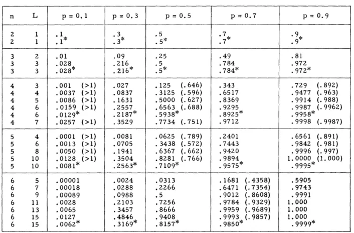
Numerical values of S(n) are included in Appendix I for comparison with upper bound expressions.

The results expressed in Eqs. 8a and 8b are for perfect nodes (t=l). Because of the symmetry of the complete graph, node failures are simply introduced. Let S(t, n) and W(t, n) be the probabilities of strong and weak connectivity in the n-node graph for t 1. Then S(t,n) n- S(k) (9) k=O0 n k-k W(t, n)= E (n2) tk(1 t)nk W(k) - (10) Z- k-2/ (10) k=2

Equations 9 and 10 are obtained by the disjoint-event method. For example, there are (k) possible sets in which k nodes are present and n - k nodes are destroyed. The k nodes that are present form a complete graph that is strongly connected, with a prob-ability S(k). Likewise, there are k-2) possible sets of nodes in which k nodes, including the terminal nodes of the desired path, are present. A path exists between the terminal nodes with probability W(k) = P1 2.

3.2 A SYNTHESIS PROBLEM

An interesting question in probabilistic-graph synthesis is the following (assume node reliability t = 1): What arrangement of L-links maximizes the probability of a path between two (terminal) nodes, if no parallel links are permitted? The constraint against parallel links prevents the trivial solution of placing all L-links directly between the terminal nodes. Clearly, the optimum olutions for L = 1, 2, 3, 4, 5, 6, and 7 are

I 2 (a) L=l I ) 2 (b) L=2

I

ZI77

Fig. 6. Optimum L-link graphs for maximizing P1 2.

those shown in Fig. 6 (a question might arise for L = 7, but a simple calculation shows that P 1 2 is reduced by removing the link between nodes 5 and 2 and placing it between

nodes 3 and 4, or between nodes 4 and 5).

The problem becomes more involved when we consider the 9-link graph. Should an additional parallel path of length 2 (including node 6) be added to the graph in Fig. 6g, or should the two additional links be placed between nodes 3 and 4, and nodes 4 and 5 ?

The calculation of P1 2 for this problem already becomes difficult, but after it is made,

it shows the parallel-path arrangement best for all values of link reliability, p. It may now appear plausible that when L is odd, the use of parallel paths of length 2 is

opti-mum. Let us consider this possibility in detail. It can be seen from Eqs. 4 and 5 that for p very small, P1 2 behaves as

P12 = P + AsP p<< 1

and for p very close to 1, P1 2 behaves as

P12 = 1-B qm_{12 m} q << 1 (I lb)

where s is the length of the shortest path between nodes 1 and 2 (not counting the direct link); As is the number of such paths; m is the size of the smallest minimal cutset; and

s

15

(lla)

__ ______

Bm is the number of such minimal cutsets. Thus, for p close to 0, P1 2 is maximized

by making s as small, and As as large, as possible. Both conditions are met for L odd

by setting s = 2 (only one path of length 1 is allowed) and As = (L-1)/2, that is, by using

the parallel-path graph. Likewise, for p close to 1, P12 is maximized by making m as large, and Bm as small, as possible. A little thought will show that the largest m that

can be made is l+(L-1)/2, and this is attained, for L odd, by using the parallel-path graph. Any other arrangement that satisfies the constraint against parallel paths will have a smaller m, and thus a smaller P1Z for sufficiently small q, irrespective of the

relative sizes of the Bm 's. Thus, for very small p and very large p, the parallel-path graph is optimum when L is odd.

The range of p for which the parallel-path graph is optimum is extended by the fol-lowing theorem.

THEOREM: The parallel-path graph is optimum for p > l1/.i when L is odd.

Before proving this theorem, let us consider the possible alternatives to the parallel-path graph. One arrangement would be that illustrated in Fig. 7a, in which every node has a direct connection to both terminal nodes, but in which there are additional "center" links spanning nonterminal nodes. It is obvious that graphs of the form of Fig. 7a are better than those of Fig. 7b. Nevertheless, a general proof of this obvious statement - as evidence of the difficulty of working with probabilistic graphs - is still not available.

The proof of the theorem involves obtaining an upper bound on P1 2 that applies to all

possible L-link graphs with h center links, and then showing that this upper bound is less than the P1 2 for the L-link parallel-path graph, when p >- 1//. The upper bound

is obtained by applying the factoring technique to all h center links of the graph. Thus, P1 2 is expanded in the form

h (m)

P12 =

Z

q

m=O z=1

where each term p q Wz(m) represents the contribution to P1 2 of the disjoint event

obtained by shorting a particular set of m center links and opening the remaining h - m center links. (A link is shorted by superimposing its two terminal nodes. A link is opened by removing it from the base graph. See section 2. 2.) There are ( h) possible ways of selecting these m links from the set of h, and, for convenience, we assign to each way a number 1, 2, (mh). h., In the term considered in Eq. 12, Wz(m) is the

th z

probability of a path in the graph obtained by shorting the z set of m links. Note that the factored graph has the form of Fig. 8a or 8b, if the unfactored graph had the form of Fig. 7a or 7b, respectively.

Let us obtain an upper bound on Wz(m) for the factored graph of the type shown in Fig. 8b (which includes the graph of Fig. 8a as a special case). Consider each of the j paths joining left and right terminal nodes, other than the single link, and number them

(a)

(a)

(b) (b)

Fig. 7. Possible graph configurations.

log (I-q b )

Fig. 8. Graph configurations after factoring.

log (I-qX)

b c

x

(I-qr)]

Fig. 9. Inequality resulting from concaveness of log (1-qX).

17

~I

from top to bottom 1, 2, ... , j. Let c1 and r denote the number of links between left

and center nodes, and between center and right nodes, respectively, in path i(l<i_j). Note that c + c2 +... + c = C and r1 + r2 +... + rj = R, where both C and R are

independent of the particular factoring considered, and depend only on the total number of links leaving the left and right terminal nodes, respectively.

Now consider the probability, B(c, r), that a path with c left links and r right links is not broken. For convenience, call such a path a (c, r)-path. Clearly, B(c, r) is the product of the probabilities that the left and right terminal nodes are both connected to the center. Thus

B(c, r) = (-qC)( 1-qr) (13)

Now, let b = (c+r)/2. We claim that

B(c,r) (-qb) 2 (14)

To prove Eq. 14, it is sufficient to show that the following inequality is true, since the logarithm is a monotonic increasing function of its argument. Therefore

log ( -q ) -[log( 1-qC ) +log ( -q r ) (15)

However, log (1-qx) is a concave downward function of x. This property is sufficient to prove Eq. 15, as can be seen from Fig. 9. Note that the equality holds if and only if r = c = b, a case that would exist if the factored graph were of the type shown in Fig. 8a.

Now, let us write the probability, Wz(m), for the factored graph of Fig. 8b. Since a path exists between nodes 1 and 2, unless all connecting paths are broken, it is clear that

Wz(m) = 1 - {q[1-B(cl, r)] ... [1-B(c., r)] j (16)

Therefore, by substituting from Eq. 14 in Eq. 16, we obtain

W,(m) - I )I- 1 - qi)]} (17)

Performing the squaring operation, and introducing our definitions of R and C, we obtain, from Eq. 17,

Wz(m) -< 1- i qR+C~2·+1

i-:i[-W (m) S I _ {qR 2 [2-q ₂ qb ... 2-q J} (18)

Thus, the probability of a path in a factored graph obtained from a particular set of m shorted center links and h - m opened center links is bounded above by the right-hand side of Eq. 18.

Let us obtain a weaker, but more general, upper bound on Wz(m) that depends only on m, and not on z. First, consider the factored graph of Fig. 8b. Note that to obtain a (c, r)-path, it is necessary to use at least d = [max(c,r)-1] shorted links. For example, suppose c r. The c links from the left terminal are required to connect with c different center nodes in the unfactored graph (on account of the constraint against parallel links), and for these c-nodes to be superimposed in the factored graph, a mini-mum of c-l links must be shorted. Thus, d = c-l.

We are now in a position to generalize the upper bound on Wz(m). Consider the log-arithm of the bracketed terms in Eq. 18:

log (-qbl) + log (2-qb 2) + ... + log (z-q b j) (19)

Again, log (Z-qX) is a concave downward function. Since the sum of the bi's is constrained to be B, an argument similar to that for Eq. 15 shows that the sum in Eq. 19 is mini-mized by making one bi, say b1, as large as possible at the expense of all other bi's.

That is, if bl can be increased by decreasing, say b2, then the change should be made,

because it decreases the sum in Eq. 19. This change is accomplished by moving a shorted link from the group of nodes forming the b2-path to the group of nodes forming

the b -path, and using this additional shorted link to superimpose an additional path on the bl-group. This process is illustrated in Fig. 10; the graph in Fig. 10b has a better path probability than that in Fig. 10a.

PATH I

I 2 2

PATH 2

(a) Fig. 10. Increase of P1Z by exchange of shorted link, P1 2(b) > P1 2(a).

42

(b)

The end of this improvement process is reached when all m shorted links have been switched to path 1. From our earlier discussion, the largest that b can then be is m + 1, and this is achieved in an (m+l, m+l)-path for which d = (m+l) - 1 = m. For, if b1 were any larger, then the minimum required number of shorted links, d, would be

greater than the available number m, which, of course, is not possible. Now, Wz(m)

is maximized by having all remaining bi's equal to 1; that is, by having all remaining paths be parallel paths of length 2 [(1, 1)-paths] for which d = 0. The number of such paths is obtained by using the constraint equation on the sum of the bi's.

bl + b + ... bj = B = (R+C)/2 (20a)

Thus, if B is an integer, the number of (1, 1)-paths is B-bl = B-(m+l). However, if B is not an integer, all bi's (i#l) can not be set equal to 1, because an even number of links is not available. One b1 must equal 1/2. In either case, the sum b2 + b3 +... + bj

is equal to B-(m+l). Hence

b2 + b3 + ... + bj = B-(m+l) (20b)

Thus, with the use of Eqs. 18 and 20b, and of the fact that b1 = m+l, the upper bound

on Wz(m) becomes

W (m) -qB+[2-qm+l ][2-q]B-m-l (21)

and this upper bound is independent of z. The upper bound in Eq. 21 can be achieved by a factored graph if the original graph is of the type shown in Fig. 7a, and m B-1. This optimal graph has 1 (m+l, m+l)-path and B-(m+l) parallel paths of length 2 [(1, 1)-paths].

We can now substitute Eq. 21 in Eq. 12 and obtain an upper bound on P12

h < pm qh-m{lqB+l[2_qm+l[2q]B-m- (22)

m=0 z=1

However, since the terms in the sum are independent of z, Eq. 22 becomes

P12 (h) pm qh-m{lqB+1[2 qm+l][2_q]B-m-l} (23)

m=O

The summation on m can be performed, and yields as an upper bound

P1 2 < 1-qB+l (2-q) B-h-[2(l+pq)h q(q+2pq)h] (24)

We can now complete the proof of the theorem by demonstrating that the upper bound given by Eq. 24 is less than the path probability, P 2, in a parallel-path graph with the

same number of links, L, when L is odd and p > 1//2. An exact expression for PI2 is obtained by noticing that a path does not exist only if all parallel paths of length 2 are broken, as well as the single direct link. Therefore

P1 = 1-q( lp2) (L- 1)/2 (25)

Now, the number of links in the graph with center links is equal to the sum of the direct link, the links touching the right and left nodes, and the h center links. That

is,

L = 1 + C + R + h = 2B + h 1 (26)

Equation 25 can now be written

P~ = l-q(l-p2)B+h/2 = 1-qB+l+h/Z(2-q)B+h/2 (27)

From Eqs. 24 and 27, we see that P12 is greater than the upper bound on P1 2 if

qh/2(Z-q)h/2 ,< (-q) - h- 1 [Z(l+pq)h-q(q+pq)h

]

or

(Z-q)[q(2-q)3]h/2 < 2[(l+pq)2]h/2 - q[(q+2pq)2]h/2 (29)

Now, inequality 29 is satisfied if the two following inequalities are satisfied:

q(2-q)3 (1+pq)2 (30)

q(2-q)3 > (q+2pq)2 (31)

But inequality 31 is always true, because it can be rewritten [with (2-q) = (l+p)] as

q(l+p)(l+p) > q(l+p-2p 2)(l+2p) (32)

and each of the factors on the left-hand side is greater than or equal to the corresponding factor on the right-hand side. Furthermore, multiplying both sides of Eq. 30, and simplifying, we obtain

-(l+2p+p2 ) < -(2+2p-p 2) (33a)

or

Zp2 _1 > 0 (33b)

which is satisfied if p 1/v2. Hence this condition, p > 1/v/, is sufficient to guar-antee the inequality in Eq. 29, and thereby the validity of the theorem.

The question might arise as to whether or not it is necessary that Eqs. 30 and 31 both be satisfied, in order that Eq. 29 be true. The answer, of course, is no. However, if the inequality in Eq. 30 is not true (i.e., p < 1//2), then there is a sufficiently large value of h for which inequality 29 is not true. The proof of this statement follows from the fact that if a > b, then there is some sufficiently large value of h, so that for any numbers A and B (even A << B) we can have

A ah > B bh (34)

Thus, either our upper bound, Eq. 24, is too weak, or better configurations exist than the parallel-path graph, when the number of nodes and links becomes large.

One might hopefully attempt an argument of this kind. Since the parallel-path graph is best for very small p, and also for p > 1/_/, then it must be best for all p. That is, we could argue that the path probabilities exhibited in Fig. 11 are not both possible.

--- PATH LENGTH =J I 0 (al U br-,i I PATH LENGTH = k (b) GRAPH Tr

Fig. 11. P1 2 as a function of p for Fig. 12. Possible pair of graphs for obtaining

the curves of Fig. 11.

two graphs.

However, this argument is not valid. Two graphs can be constructed whose path prob-abilities cross as often as desired, and at any desired places. For example, consider two graphs made up of disjoint parallel paths (see Fig. 12). Graph I has one path of length 1 and three paths of length j. Graph II has two paths of length 2 and one path of length k > 1. Thus Graph I has a higher value of P1Z for small p, since the path of length 1 dominates, and has a higher value of P_{1 2} for large p, because the smallest cutset contains a number of links equal to the number of paths, and the number of paths is greater (by 1) for Graph I. But Graph II can be made to have a higher value of P1 2

for a certain range of p by proper choice of j. Consider the following inequality.

(lp ) <l-p)(1 -p j ) ₍₃₅₎

The left-hand side of the inequality is an upper bound on (-P 1 2) in Graph II, obtained

by ignoring the contribution of the k-length path; the right-hand side of the inequality is (1-P 1 2) in Graph I. Since (-p )2 < (l-p) (for p = 3/4, for example), it is obvious that

j can be made sufficiently large that Eq. 35 is satisfied. Thus, the graphs of Fig. 12 can yield path probabilities P1 2 that behave with p as shown in Fig. 11. Also, the

rela-tive number of links between the two graphs has no influence because, if k = 2, Graph I has more links than Graph II, whereas if k = 3j, Graph II has more links than Graph I, and the previous results are not disturbed in either case. From this discussion, it should be clear that as many crossings can be obtained as desired, at values of p arbitrarily close to specified values, by building graphs with disjoint paths of various lengths con-taining various numbers of links in parallel.

22

A final result can now be shown concerning our synthesis problem. We can derive a ratio of the number of center links to the total number of links that must be satisfied if the center-link graph is to have any possibility of being better than the parallel->3=5~-L path graph. This ratio is obtained by using

2 / the fact that the probability of a path in a graph with C-links touching the left node,

C LINKS R LINKS

and R links touching the right node, is Fig. 13. Graph configuration for upper bounded above by the probability of a path

bound on P12 in the graph shown in Fig. 13 (the direct link between the terminal nodes is disre-garded in this discussion). The probability of a path in the graph of Fig. 13 is

P1 2 = (1-qC)(1-qR) (1-qB)2 (1-qB) (36)

in which the inequality of Eq. 14 has been used. A condition under which the upper bound in Eq. 36 is less than the exact P'2 for the parallel-path graph is obtained as follows:

12 (1-qB) < 1- (1-p2)(L- 1)/2 = P 1Z if B log q 1 log (1-p) or R+C _a- log (1-p2) _{= 1-} log (1+p) ₍₃₇₎ L-1 log q log 1/q

Equation 37 can be written in terms of the number of center links, h, with h = (Ll) -(R+C). Then

log (l+p)

h < (L-1) (38)

log (1/l-p)

Thus, for any value of p, there is a definite upper bound on the fraction of links that may be used as center links in an optimum graph, although for p close to zero the fraction approaches 1.

3.3 AN UPPER BOUND ON THE PROBABILITY OF STRONG CONNECTIVITY

The form of the graph-factoring equation, stated in section 2. 2 and repeated in Eq. 39, suggests the possibility of obtaining an upper bound on the various connectivity probabilities in terms of a difference equation (when t = 1). In this section the difference equation is solved with boundary conditions appropriate to S, the probability of strong

connectivity [cf. (12)]. Properties of the solutions are determined, and an alternative derivation is made.

The graph-factoring equation is

S = qS₁ +pS ₂ (39)

where S1 and S2 are the probabilities of strong connectivity in graphs resulting from

opening and shorting a particular link in the original base graph. Now, consider all pos-sible n-node, L-link graphs. Since there are only a finite number, S must take on a maximum value among them. Call this maximum, Pl(n, L). We shall obtain an upper bound, P2(n, L), so that for all n, L,

Pl(n, L) P2(n, L) (40)

Let us apply Eq. 39 to an optimum graph, which has S = Pl(n, L), to obtain an upper bound on P1.

P 1(n, L) -< q Pl(n, L-1) + p P1(n-1, L-1) (41)

The right-hand side of Eq. 41 may be larger than the left-hand side for two reasons. First, the opening of a link in an optimum n-node, L-link graph may not result in an optimum n-node, (L-1)-link graph, and so the use of Pl(n, L-1) is optimistic. Second, the shorting of a link in the n-node L-link graph may result in a graph with less than

L-1 links if and only if there are links in parallel with the shorted link. Thus, the assumptions that L-1 links remain, and that the arrangement of the L-1 links among the remaining n- nodes (two nodes have been superimposed) is optimum, are both optimistic.

The upper bound on Pl(n, L) in Eq. 41 is further enhanced if we substitute P2 for P1

on the right-hand side. We then have

P1(n, L) < q P2(n, L-1) + p P2(n-1, L-1) (42)

From Eq. 42, we see that Eq. 40 is satisfied if we define P2(n, L) as the right-hand side

of Eq. 42. Thus

P2(n, L) = q P2(n, L-l) + p P2(n-1, L-1) (43)

Equation 43 thus defines Pz(n, L) as a difference equation. In order to solve explicitly for P2(n, L), it is necessary to introduce boundary conditions. The boundary conditions

that we shall use are:

P2(2, L) = P1(2, L) = I - qL (44)

n-1

P2(n, n-l) = Pl(n, n-l) = (45)

In Eq. 44, P1(2, L) is obtained from the fact that the optimum arrangement of L-links

among two nodes is achieved by placing all links in parallel (clearly, slings do not help). Then the graph is strongly connected if at least one link is present. Equation 45 is obtained from the fact that if only n-l links are present in an n-node graph, then the graph can be strongly connected if and only if all links are present.

Equation 43 can now be solved with the help of the boundary conditions, Eqs. 44 and 45. The solution is

n I L-n+l n+k-2 k

P2(n, L) = pn - n+k-2) q; ( n > 2, L n-1 (46)

k=0

First, note that Eq. 46 satisfies both boundary conditions. Then, to show that Eq. 46 satisfies Eq. 43, substitute it in Eq. 43 and simplify. This procedure yields

L-n+l ( k ) [( kkl ) (n+k

n-1 L+ I n+kZ) k n-l L-+ [(n+k-3) + (n+k-3)] (47)

p

Z

q

p

y

n 3 +

q

(47)

k=0 k=0

where, by convention, (1) = 0. Equation 47 is an identity if

(n+k-2) = n+k-3) + (n+k- 3)(48)

which is a well-known recursion for binomial coefficients [see, for example, Riordan(23)]. Several properties of P2(n, L), as defined explicitly by Eq. 46, are of interest. First,

we should note that as L tends to infinity, for any fixed n, the sum on the right-hand side of Eq. 46 approaches (l-q) (n 1), and hence P2(n, L) tends to 1 from below.

Next, note that the coefficients, ak(n), of q can be obtained rather simply from Eq. 48. Table 1 is constructed by writing for each entry the sum of the entry directly above it and the entry directly to the left of it.

We shall now determine the conditions under which P2(n, L) is an attainable upper

bound; that is, the conditions for which P2(n, L) = Pl(n, L). First, recall that if P2(n, L)

is actually the probability of connectivity in an n-node graph, then the coefficient of

n-1

p in a Taylor-series expansion of P2(n, L) about p = 0 must equal the number of trees

Table 1. Coefficients of qk in Eq. 46.

n ao(n) al(n) az(n) a₃(n) a₄(n) a₅(n) a₆(n)

2 1 1 1 1 1 1 1 3 1 2 3 4 5 6 7 4 1 3 6 10 15 21 28 5 1 4 10 20 35 56 84 6 1 5 15 35 70 126 210 7 1 6 21 56 126 252 462 25