A Computational Investigation of the Fluid
Dynamics of a Three-Dimensional,
Compressible, Mixing Layer with Strong
Streamwise Vorticity
by
Jonathan Kindred Elliott
B.A.I. Mechanical Engineering, B.A. Mathematics, Trinity College, Dublin (1987)
SUBMITTED IN PARTIAL FULFILLMENT OF THE REQUIREMENTS FOR THE DEGREE OF
Master of Science
Aeronautics and Astronautics
at the
Massachusetts Institute of Technology June, 1990
@Massachusetts
Institute of Technology 1990Signature of Author . . -
-Department of Aeronautics and Astronautics February, 1990
Certified by
Dr. Choon S. Tan Thesis Supervisor
Accepted by
AcceptedbyProfessor Harold Y. Wachman Chairman, Departmental Graduate Committee
MASSACHUSETTS INSTITUTE OF TECHNOLOGY
JUN
19 1990
UBRACH8b
A COMPUTATIONAL INVESTIGATION OF THE FLUID DYNAMICS OF A THREE-DIMENSIONAL, COMPRESSIBLE, MIXING LAYER WITH
STRONG STREAMWISE VORTICITY by
Jonathan Kindred Elliott
Submitted to the Department of Aeronautics and Astronautics in June 1990 in partial fulfillment of the
requirements for the Degree of Master of Science in Aeronautics and Astronautics
Abstract
A three-dimensional Euler solver employing Zalesak's multidimensional flux-limiter in a Flux-Corrected Transport (FCT) algorithm has been developed and used for the analysis of flow phe-nomena in a three-dimensional lobed mixer. In particular, results from the computed flow in a subsonic low penetration mixer, a supersonic low penetration mixer, a subsonic high penetration mixer and a supersonic high penetration mixer are used to investigate the effects of compressibility and lobe geometry on the generation of streamwise vorticity and the subsequent downstream evo-lution of the vortex sheet. The main results of this work are: (1) over the range of Mach numbers examined (M < 2.0) compressibility has only a marginal effect on the generation and evolution of the vortex sheet, (2) the dependence of the secondary circulation on the geometry can be estimated through the use of the simple scaling law developed by Barber, Paterson and Skebe in [3], and (3) the vortex sheet shed from the mixer lobe trailing edge exhibits a tendency to roll-up into a discrete, approximately circular, vortical region.
Acknowledgements
I would first like to thank my advisor, Dr. Choon Sooi Tan, for being a constant source of inspiration and encouragement during the course of this project. The effort he put into editing the thesis was greatly appreciated even though at times it may have seemed that this was not so. My thanks also go to Professor Greitzer for his encouragement, the incisiveness of his comments throughout and for the fine job of editing that he did. The contributions of Professor Frank Marble to the fluid dynamic aspects of the research were also invaluable.
My friend and colleague in lobed mixer research, Yuau Qiu, deserves special mention for the hours of discussions and for running the Trefftz plane calculations.
Thanks are certainly in order to the following people from the Laboratory for Computational Physics in the Naval Research Laboratory: Stephen Zalesak, for the hours of consultative advice on the details of the multidimensional FCT algorithm; Elaine Oran, for providing the LCPFCT subroutine and other software; Fernando Grinstein and Gopal Patnaik for their helpful discussions concerning the LCPFCT algorithm.
Thanks also to Nikolaos Gatsonis for arguing the advantages of using Zalesak's implementation and for providing the two-dimensional, Cartesian flux limiter and his other advice on the numerics. I would also like to mention some of the GTL crowd: karl Renaud, for help with computer and fluid dynamic aspects; Dan Gysling; Pete Silkowski; Andreas Schulmeyer; Eric Strang; Rob Plumley; Seung Jin Song; Bill Steptoe; George Pappas.
This project was supported by the Naval Air Systems Command, under NAVAIR Contract N00019-88-C-0229, project manager, George Derderian. Support for the author was provided by the Air Force Research in Aero Propulsion Technology (AFRAPT) program, AFOSR-85-0288 E. This support was greatly appreciated.
Contents
1 Introduction
2 Computational Algorithm
2.1 Finite Volume Discretization of the Euler Equations ... 2.2 Flux-Corrected Transport ...
2.3 One-Dimensional Boris-Book FCT ...
2.4 Zalesak's Extension of Boris-Book FCT to Multidimensions 2.5 Zalesak's Fully Multidimensional Flux Limiter . . . . 2.6
2.7 2.8
High Order Scheme ... Low Order Scheme ... Boundary Conditions ...
2.8.1 Farfield Boundary Conditions ... 2.8.2 Solid Body Boundary Conditions ...
3 Development of the Numerical Algorithm for the 3.1 Flow in a Channel over a Circular Arc Bump . . .
3.1.1 Supersonic Circular Bump ... 3.1.2 Transonic Circular Bump ... 3.1.3 Subsonic Circular Bump ...
3.1.4 Summary of the Computed Results for Ni's 3.2 Planar Shear Layer Calculations ...
3.2.1 Timestep-Splitting Calculations ... . . . . 25 . . . . 27 . . . . . 32 . . . . . 34 . . . . . 38 . . . . 41 . . . . 43 . . . . . 43 . . . . . 45 Implementation of FCT Bump
3.2.2 Finite Volume Calculations ...
3.2.3 Summary of Two-dimensional Shear Layer Calculations . . . .
4 Lobed Mixer Calculations
4.1 Further Details of the Numerical Scheme . . . . 4.2 Grid Generation Algorithm ...
4.3 Low Penetration Mixer: Subsonic Calculation . . . 4.4 Low Penetration Mixer: Supersonic Calculation . . 4.5 High Penetration Mixer: Subsonic Calculation . . . 4.6 High Penetration Mixer: Supersonic Calculation 4.7 Summary ... . . . . 95 . . . . . 98 . . . 106 . . . . .109 . . . 113 . . . ... 115 5 -Conclusion 5.1 Development of the Numerical Scheme . . . . 5.2 Fluid Mechanics of the Lobed Mixer . . . . 6 Recommendations for Future Work 6.1 Improvement of CFD Algorithm ... 6.2 Physical Aspects ... 63 63 166 S. 166 . . 167 168 .. 168 .. 170
List of Figures
1.1 Typical lobed mixer ... 20
1.2 Lobed mixer as found in a turbofan ... 20
2.1 Typical cell face showing vectors si, s- used to find S ... . . ... 47
2.2 Typical cell showing vectors t, t, t] used to find V ... . . . . 47
2.3 The eight possible configurations of the wtd in the neighbourhood of a positive an-tidiffusive flux A,+1/2. (Taken from Zalesak) ... .... . . 48
3.1 Grid with 10% thickness circular arc bump used for subsonic calculation ... 64
3.2 Grid with 10% thickness circular arc bump used for transonic calculation ... 64
3.3 Grid with 4% thickness circular arc channel used for supersonic calculation ... 65
3.4 Isomach contours for supersonic calculation by High Order Scheme ... 66
3.5 Mach Number Distribution along the lower wall as calculated by the High Order Scheme for supersonic inflow ... 66
3.6 Total pressure contours for supersonic calculation by High Order Scheme ... 67
3.7 Isomach contours for supersonic calculation by Low Order Scheme ... 68
3.8 Mach Number Distribution along the lower wall as calculated by the Low Order Scheme for supersonic inflow ... 68
3.9 Total pressure contours for supersonic calculation by Low Order Scheme ... 69
3.10 Isomach contours for supersonic calculation by FCT Scheme ... 70
3.11 Mach Number Distribution along the lower wall as calculated by the FCT Scheme for supersonic inflow ... ... .. 70
3.13 Density contours for supersonic calculation by FCT Scheme ... 72 3.14 Density Distribution along the lower wall as calculated by the FCT Scheme for
supersonic inflow ... . . . .... 72 3.15 Isomach contours for transonic calculation by High Order Scheme ... 73 3.16 Mach Number Distribution along the lower wall as calculated by the High Order
Scheme for transonic inflow ... ... 73 3.17 cp contours for transonic calculation by High Order Scheme ... 74 3.18 c, distribution along the lower wall as calculated by the High Order Scheme for
transonic inflow ... ... 74
3.19 Total pressure contours for transonic calculation by High Order Scheme ... 75 3.20 Isomach contours for transonic calculation by FCT Scheme ... 76 3.21 Mach Number Distribution along the lower wall as calculated by the FCT Scheme
for transonic inflow ... . ... 76 3.22 cp contours for transonic calculation by FCT Scheme ... 77 3.23 cp distribution along the lower wall as calculated by the FCT Scheme for transonic
inflow ... .... . ... .. ... . .. ... .. . ... . ... . 77 3.24 Total pressure contours for transonic calculation by FCT Scheme ... 78 3.25 Isomach contours for transonic calculation by Low Order Scheme ... 79 3.26 Mach Number Distribution along the lower wall as calculated by the Low Order
Scheme for transonic inflow ... 79 3.27 Total pressure contours for transonic calculation by Low Order Scheme ... 80 3.28 Isomach contours for subsonic calculation by High Order Scheme ... 81 3.29 Mach Number Distribution along the lower wall as calculated by the High Order
Scheme for subsonic inflow ... 81 3.30 Total pressure contours for subsonic calculation by High Order Scheme ... 82
3.31 Isomach contours for subsonic calculation by Low Order Scheme ... 83
3.32 Mach Number Distribution along the lower wall as calculated by the Low Order Scheme for subsonic inflow ... 83
3.33 Total pressure contours for subsonic calculation by Low Order Scheme ... . 84
3.34 Isomach contours for subsonic calculation by FCT Scheme ... 85
3.35 Mach Number Distribution along the lower wall as calculated by the FCT Scheme for subsonic inflow ... ... .. 85
3.36 Density contours for subsonic calculation by FCT Scheme ... 86
3.37 Density Distribution along the lower wall as calculated by the FCT Scheme for subsonic inflow . . ... . .. .. . ... .. . .. . .. . . . . .. . .. .. . . . ... 86
3.38 Total pressure contours for subsonic calculation by FCT Scheme ... 87
3.39 Grid used for subsonic planar shear layer calculations ... 88
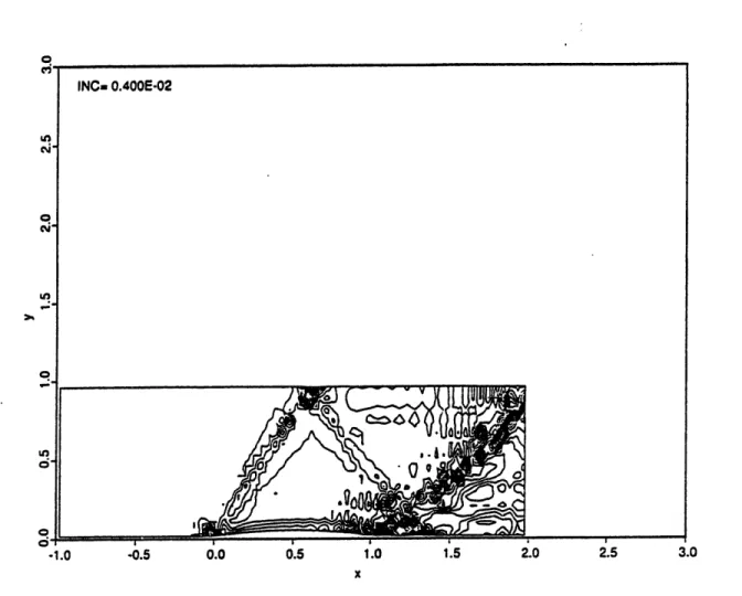
3.40 Passive scalar,
i
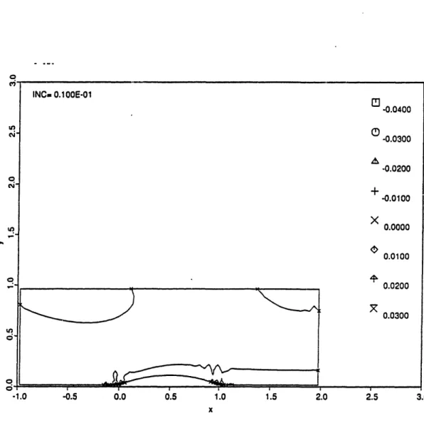
= jor+Nr at various stages in the evolution of the subsonic instability . . . 893.41 Vorticity at various stages in the evolution of the subsonic instability ... . 89
3.42 Passive scalar, = Noer, at various stages in the evolution of the supersonic instability . . . .... . . 90
3.43 Passive scalar, i/= ower+Npp at various stages in the evolution of the instability Nower +Nppe.r as calculated by FVFCT ... 91
3.44 Vorticity at various stages in the evolution of the instability as calculated by FVFCT 91 4.1 Comparison of limiters ... 117
4.2 Low penetration mixer: (a) isometric view; (b) front elevation ... 118
4.3 High penetration mixer: (a) isometric view; (b) front elevation ... . 119
4.4 Low penetration mixer grid ... 120
4.6 Convergence history for subsonic low penetration mixer case ... 122
4.7 vy contour plot ... ... 122
4.8 Spanwise velocity vector field ... ... 123
4.9 Secondary velocity vector field at an axial location 0.02A downstream of the lobe trailing edge ... ... 123
4.10 vy contour plot as found by UTRC investigation ... . 124
4.11 Secondary velocity vector field as found by the UTRC experimental investigation . . 124
4.12 vy profile as found by UTRC investigation ... ... 125
4.13 Contour plots of cp, vy and vz... 126
4.14 axial variation of cP~p,, and Cplow,... ... 127
4.15 Circulation versus spanwise distance at lobe trailing edge. ... 128
4.16 Loading cpppe, - Cpowe on lobe surface projected onto a y = consant surface . ... 128
4.17 Compressible Bernoulli Equation residual ... ... 129
4.18 APt contour plot ... 130
4.19 APt/Poo plot in mixing duct ... 131
4.20 Secondary velocity vector field at axial locations x/A = 3.02, 11.06, 18.71 ... 132
4.21 Circulation variation with axial distance ... ... 132
4.22 Contour plots of
k,
aw, and cp ... ... 1334.23 Length of O = 0.5 contour versus axial distance for subsonic low penetration calculation 134 4.24 Comparison of ip contour plots at an axial location 4A downstream of the lobe trailing edge as calculated by 3-D FCT method (left) and Trefftz plane method ... 135
4.25 Comparison of 0 contour plots at an axial location 9A downstream of the lobe trailing edge as calculated by 3-D FCT method (left) and Trefftz plane method ... 135
4.26 Comparison of cp contour plots at the lobe trailing edge as calculated by 3-D FCT method (left) and Trefftz plane method ... 136
4.27 Convergence history for supersonic low penetration mixer case ... . . . 136
4.28 Contour plots of cp, vy and v. ... ... 137
4.29 Contour plot of APt/P, around lobed mixer ... ... 138
4.30 Axial variation of cppp,•and Cplow,,r... ... 139
4.31 Loading on lobe surface for supersonic case ... .... 139
4.32 Contour plot of cp at spanwise location adjacent to the symmetry boundary ( = 1) 140 4.33 v,/U contour plot for supersonic lpm case ... ... . . 140
4.34 vy/U profile for supersonic lpm case ... ... 141
4.35 Circulation versus spanwise distance at lobe trailing edge for supersonic low pene-tration calculation ... . ... 141
4.36 APt/Poo
...
142
4.37 Secondary velocity vector field at axial locations x/A = 3.02, 11.06, 18.71 ... 143
4.38 Circulation variation with axial distance for supersonic low penetration calculation . 143 4.39 Contour plots of , w, and cp ... 144
4.40 Interface length versus x for lpm supersonic case ... . 145
4.41 Convergence history for subsonic high penetration mixer case ... 146
4.42 Pt contour plot ... ... 147
4.43 vy profile as found by UTRC investigation ... ... 148
4.44 Contour plots of cp, vy and v. ... 149
4.45 Axial variation of cp,,,, and Cpto,•,... ... 150
4.46 Loading cp.pp,, - cpor., on lobe surface projected onto a y = consant surface . ... 151
4.47 Compressible Bernoulli Equation residual ... ... 152
4.48 Circulation versus spanwise distance at lobe trailing edge. ... 152
4.49 Circulation variation with axial distance ... ... 153
4.51 Contour plots of , w. and cp ... 154
4.52 Secondary velocity vector field at axial locations z/A = 1.52, 5.51,9.74 ... 155
4.53 Length of 0 = 0.5 contour versus axial distance for subsonic high penetration calcu-lation ... 156
4.54 Convergence history for supersonic high penetration mixer case ... 156
4.55 Pt contour plot ... ... 157
4.56 Contour plot of p at z = 0 ... 157
4.57 transverse profiles of p at z = 0 ... 158
4.58 Contour plots of cp, vv and v. ... 159
4.59 axial variation of cp,,,,, and Cpowc . . . 160
4.60 Loading cp.ppe, - cploe,, on lobe surface projected onto a y = consant surface. 12 Contours are plotted from -0.55 to 0.55 in increments of 0.05 ... 161
4.61 Circulation versus spanwise distance at lobe trailing edge for high penetration su-personic case .... .... ... ... . . ... .. .. . ... . ... 162
4.62 Circulation variation with axial distance for high penetration supersonic case. .... 162
4.63 APt/PO plot in mixing duct ... 163
4.64 Secondary velocity vector field at axial locations x/A = 1.52, 5.51 ... 163
4.65 Contour plots of 0, w2 and cp ... 164
4.66 Length of = 0.5 contour versus axial distance for supersonic high penetration calculation ... ... .... .. 165
Nomenclature
at
a, b
A
Amplitude of mixer
Exponents in grid generation forcing terms
Antidiffusive flux
c Sound speed
c Complex phase velocity, c, + ici
c, Pressure coefficient, (P - P-oo)/pUool
cp, ,c Specific heat at constant volume and pressure
C Fraction that multiplies antidiffusive flux
Cz, Cz, etc. Coefficients used to implement solid wall boundary condition
e,
f,
g Inviscid flux vectorse,, f,, g, Source components of the inviscid flux vectors
Et Total energy per unit volume
Ei+i ,j,k Inner product of flux vectors with area vector on ý faces ((e, f,g) S)i+L,i,kAt.
Fi,i+ ,k Inner product of flux vectors with area vector on r faces ((e, f, g) - )i,i+),k Gidk+• Inner product of flux vectors with area vector on ý faces ((e, f,g) S)i,,k+At.
G Amplification factor
Ho Total Enthalpy
J Jacobian of the transformation from physical to computational space 10
kD Transport coefficient for diffusion of molecules
km Wave number
L Length scale characteristic of transverse variation of basic current
Lm Mixer length
Le, L,, Lr Time integration operation in the e-, n- and - directions for directional timestep
splitting.
M Mach number
ii Unit normal vector (nz, ny, nz)
N Molecular number density
P Pressure
P, Q Grid generation forcing terms
Pt Total pressure
P-, P+ Sum of all andiffusive fluxes leaving/into cell (i, j, k)
Q-, Q+
Maximum allowable decrease/increase in w at cell (i,j,
k)r+, r- Riemann invariants
R-, R+ Least-upper-bound on fraction that must multiply all antidiffusive fluxes leaving/into cell at (i,
j,
k)s Entropy
S Cell face area
t Time
T Temperature
TE Truncation error
iV Velocity vector (v2, VY, Vz)
V Contravariant velocity
V Cell volume
V Velocity scale characteristic of transverse variation of basic current, Vupper - Vlower
V
Mean axial velocity, l(Vupper + Vlower)w Typical scalar w State vector x, y, z Cartesian coordinates a Disturbance wavelength a 741obe•> 74duct 7
Lobe penetration angle
Shock angle
Ratio of specific heats
Coefficients for fourth order artificial diffusion Spanwise gradient of circulation,
ar/as
r
Circulation
r* Nondimensional circulation, _. As Incremental distance At Size of timestepAx
Xi+!-
X_ 1
2 2E Internal energy per unit volume
e Local Courant number
E Relative error in grid generation scheme
e Root-mean-square state vector difference
q Disturbance amplitude
0 Deflection angle
K Coefficient of diffusion
A Lobe wavelength
y Mach angle
p Diffusion coefficient for Boris-Book limiter v Antidiffusion coefficient for Boris-Book limiter
V1, /2 Prandtl-Meyer functions
v2 Coefficient for second difference diffusion used in low order method
(, i, S Coordinates in computational space
p Density
r Circular arc thickness ratio
Sb Phase angle
q.e Exact phase angle
ik Passive scalar Niowuer/(Nupper + NMower)
wM, Y, wz, components of vorticity
wp, WQ Relaxation factors for forcing terms in grid generation scheme
Superscripts
a, b Correspond to minimum/maximum allowable value of wn+l
ad Antidiffusive
c Corrected
d Diffusive
fd Finite difference approximation
H High order
L Low order
n Temporal index
t Transported
td Transported-and-diffused
* Average of predicted and nth timelevel values
Nondimensional Predicted value Subscripts amb b face fct g high I Ambient Face at boundary Cell face Calculated by FCT scheme Guard cell
Calculated by high order scheme
Computational space indices
Cell adjacent to boundary
low Calculated by low order scheme
s Corresponding to tip of splitter plate
te Trailing edge
upper, lower Upper and lower streams
Chapter 1
Introduction
In two-dimensional shear layers, the dominant component of the vorticity vector is normal tc the velocity field. Three-dimensionality in these types of mixing layers is not a key feature of the flow and takes a long time to develop [1,39]. The basic mechanism by which mixing is achieved is through the large scale fluid motions associated with the Kelvin-Helmholtz instability and the subsequent nonlinear rollup. The only parameters that can be used to alter the mixing properties of the shear layer are related to the velocity difference (through the factor (V1 - V2)/(V2 + V1)),
the convective Mach number, M, = (VI - V2)/2a (for equal soundspeeds) and, if two different fluids are used, the density ratio, (P2/P1) and (72/71). Available experimental data and theoretical analyses [47,37] of the compressible two-dimensional shear layer, however, have demonstrated that the growth rate of the Kelvin-Helmholtz instability decreases rapidly above a convective Mach number of about 0.7 or so. Because of this, it may be difficult to obtain efficient molecular mixing of fuel and air, for example, at the supersonic Mach numbers found in a scramjet.
The purpose of lobed mixers (of which a typical geometry is shown in Figure 1.1) is to intro-duce strong streamwise vorticity into the shear layer so that the flow becomes inherently three-dimensional. The production of streamwise vorticity is achieved in a fashion analogous to its generation by a wing of finite length. As a result of the transverse penetration of the lobed mixer into the stream, the mixer lobes have a pressure difference across them and thus an associated bound vorticity. Due to the spanwise variations of the geometry, the loading and bound vorticity strength also vary in the spanwise direction, so that streamwise vortex lines, emanating from the trailing edge, must occur. Thus the lobed mixer can be viewed as the periodic juxtapositioning of a wing and an identical inverted wing. In a flow configuration where the stream on one side of the lobed mixer has a total pressure that is different from that on the other side, the resulting
downstream shear layer will consist of streamwise vorticity associated with the three-dimensionality of the mixer and spanwise vorticity associated with the variation in total pressure. The strength and distribution of the streamwise vorticity are parameters that can be used to alter the mixing properties of the three-dimensional shear layer in addition to the two-dimensional shear layer pa-rameters mentioned above. Because of this, the three-dimensional shear layers generated by lobed mixers are very different from the conventional two-dimensional shear layer.
Lobed mixers are in widespread usage in aircraft engines where one of the initial applications was for jet noise reduction. As shown for the turbofan engine in Figure 1.2, the streamwise vorticity generated by the mixer serves to mix the core and bypass airstreams such that lower effective jet velocity and shear layer intensity result. Hence an accompanying noise reduction is achieved. Lobed mixers have also been used to mix the exhaust gases from turbojet engines with the freestream atmospheric air. This also results in reduced noise level. In addition, if the stagnation enthalpies of the core and bypass streams are significantly different (whch is usually the case in turbofan engines), the mixer configuration shown in Figure 1.1 can result in thrust augmentation [2] and hence lower specific fuel consumption. There is reason to believe that the streamwise vorticity enhanced mixing observed at low Mach numbers will also be found in supersonic three-dimensional shear layers. The reasoning behind this argument is that even though flow in the streamwise direction is supersonic, the cross-stream flow is subsonic and compressibility effects may be small. The potential of lobed mixers for ejector pumping systems and as a means of improving airfoil stall margins and lift-to-drag ratios are also being investigated. Thus it is of engineering significance to develop the scientific basis for the design of optimum mixer configurations, e.g. one that produces a given mixing in the shortest length/time or maximum mixing in a given length/time, with minimum losses.
Previous research efforts include experimental investigations that established mixing is domi-nated by the secondary flow generated by the lobed mixer [4] and pinpointed the inviscid mech-anisms that create the secondary fiowfield [3]. However, in the latter case, measurements were
limited to downstream of the trailing edge with flow visualization being used on the surface of the lobed mixer. The role of the lobed mixer in mixing supersonic flow jets has also been examined [6]. Numerical investigations have been carried out for flow downstream of the lobed mixer [7,5] but these relied on experimental or other data for use as the inlet boundary conditions and the potential interaction between lobed mixer and downstream mixing duct was not modelled. Re-cently numerical investigations have been reported that generate solutions for the entire flowfield [8,9]. The first approach uses a full Navier-Stokes solver and the geometry corresponds to a specific high bypass-ratio turbofan engine. The second approach uses the two-equation x - E eddy viscosity turbulence model in the incompressible elliptic equations of fluid flow and the geometry, again, corresponds to a turbofan engine.
The research issues that need to be addressed before one can begin to develop the engineering and scientific basis for the design of an optimum mixer are:
(1) the extent to which three-dimensionality plays a role in the performance of lobed mixers as a mixing and thrust augmentation device in a propulsion system
(2) the roles of streamwise and spanwise vorticity in a three-dimensional shear layer (3) the effects of compressibility
(4) the dependence of the mixing on the trailing edge vorticity field
(5) the effects of the different geometrical parameters such as amplitude-to-wavelength ra-tio, a(z, z)/A, and mixer length L on establishing this vorticity field.
One objective of the present work was to develop a CFD tool capable of generating an accurate solution of the three-dimensional Euler equations for the flow in the entire domain, both around the lobed mixer and in the downstream mixing duct and over the subsonic, transonic and supersonic Mach number ranges. With the aid of this CFD tool, the generation of streamwise vorticity by the
lobed mixer is evaluated and the effects of compressibility on the mixing parameters are assessed. To this end, a Flux-Corrected Transoort (FCT) code using Zalesak's multidimensional flux limiter (see Section 2.5) was developed for use with three-dimensional numerical grids with general curvilinear coordinates. To the author's knowledge, it is the first implementation of Zalesak's limiter in three-dimensional curvilinear coordinates. This algorithm can handle different geometries and is capable of modelling flows with total pressure variation at inflow, although time limitations precluded the investigation of these types of flows.
The development of the numerical algorithm is the subject of Chapter Two. Two-dimensional numerical solutions for standard test cases (which capture most of the flow phenomena to be expected in the three-dimensional case) are presented in Chapter Three. Full-, three-dimensional solutions for two different lobed mixers in subsonic and supersonic freestreams are presented in Chapter Four. Chapter Five emphasises the conclusions of the investigation while the subject of Chapter Six is recommendations for future work.
Figure 1.1: Typical lobed mixer
Chapter 2
Computational Algorithm
In this chapter, the governing equations for an inviscid flow are introduced, along with their three-dimensional finite-volume discretized form. Two algorithms for their solution are presented. One is suitable for applications in which a general orthogonal numerical grid (such as Cartesian or Cylindrical Polar) can be used. The other has no orthogonality restriction and can be used with any curvilinear grid as long as the grid is structured. Both use the principle of Flux-Corrected Transport [17,18,19,21]. The first (which will be referred to henceforth as Boris-Book FCT) was developed by Boris and Book and has undergone extensive validation [17,18,19,26,27],etc. The second algorithm (which will be referred to henceforth as FVFCT (Finite Volume Flux-Corrected Transport) utilizes the principles of Zalesak's multidimensional flux limiter [21] and was developed by the author. It is the first finite volume implementation of FCT in general curvilinear coordinates that the author is aware of.
2.1
Finite Volume Discretization of the Euler Equations
The Euler equations in integral form are (from Conservation of Mass, Momentum and Energy)
f• wdV + w. adS + (es,f,,g)
.AdS
=
0
(2.1)
where, p pv 0
P
0
Pvz
J
,s 0 0P
Pv, =ar
0
0 0 P Pv,(2.2)
e,(2.3)
(2.4) and Et is the total energy per unit volume
Et =
e+
1p(v2
+ v2 + v2)(2.5)
Assuming a calorically perfect gas, the internal energy is given by
c = pcvT =- T=
--1 (2.6)
which closes the system. To put the Euler equations in conservation law form we first write them as
Ta fwdV + (e,f,g) -IdS = 0
(2.7)
where,
Using the Divergence conservation law form
pvz
2
pvz
(Et + P)v,
Theorem and the
pvy
PVYVZ
=1 pt 2 PVyVz(Et + P)v, j
fact that V is an pvz pezrz I,-g p Ivu 128pvZ
(Et + P)v,
arbitrary volume we get the familiar
8w
8e
8f
ag
09t
1=0x
(2.9)
Spatial discretization is performed using a conservative finite-volume method. This allows shocks to be "captured" without special treatment in the neighbourhood of discontinuities. This is possible because the finite-volume form discretizes the integral form of the Euler equations rather
ii=(n., ny) nz)
vV
(vzZ~ Zy~vz)
than the differential form. The integral form is applicable everywhere while the differential form is not valid in the neighbourhood of discontinuities.
The spatial discretization of Equation (2.1) based on the finite volume method reduces to a system of ordinary differential equations in the flow variables at each cell centre of the numerical grid. This numerical grid consists of a number of hexahedral cells each of which forms its own control volume around which the semi-discretized form of Equation (2.1) must be satisfied. Flow variables are defined at cell centers (i, j, k) from which the face values can be found by averaging the corresponding adjacent cell center values
1
Pi+4,,k = "+(Pij,k + Pi+1,j,k) (2.10)
(Zalesak [25] has proposed a method for increasing the spatial order of accuracy by including more cell center values in the equation for Pi+•,ik but for nonuniform three-dimensional grids, the complexities of the formulation are prohibitive and this method was not used.) As mentioned previously, the semi-discrete finite volume form is then a system of ordinary differential equations of the form
dw 1
E=
6(e,
f ,
g)face * Sface (2.11)Ft
Vk face=1or
dw 1 6
dt V.ifk (Vace• W)ace a
+
(es,f,g.)face • .face)ISfaceI (2.12)face'1
where face = 1 represents the face located at (i - ½,j, k), face = 2 that located at (i +
4,j,
k), face = 3 that located at (i,j- 1, k), etc., the unit normals are always taken to be directed outwardsand
ace - ace * face (2.13)
The normal vector A is found from
and the area vector S is found from the cross product of the displacement vectors with endpoints at the midpoints of each side of the face (see Figure 2.1)
Sface =
s
x
82
(2.15)
si = (r + rd - r - r) (2.16)
= (r + r - r-r) (2.17)
where r' is the position vector of the node located at a. The volume of cell (ij,k) is found from the vector triple product of the displacement vectors with endpoints at the midpoint of each face (see Figure 2.2) V= (t~ x t) t (2.18) (2.19) - 1 tl -" (r? + r-• + rt
+
r) - r" - r] - rl - rl) (2.19) t2=--(r÷rc +rdrh -r-r-rb -rl) (2.20) 1 t- = -(rc + rb + rf + rý - rd - rt - r - rh) (2.21)As a consistency check, it is instructive to perform the spatial discretization through the ap-plication of a generalized transformation of the Euler equations from the physical domain (x, y, z)
to the computational domain (e, rq, ). The semi-discrete form becomes (reference [28] shows the details of the manipulations)
dw 1
dt
J (((e, f,g) (Jz, JE, JCz)) + ((e,f,g) -(JOz,
J+Y,Jt1,)), +
((e,
f,
9 (J)- , Ja, Jz)) )
g)
(2.22)
where J is the Jacobian and e., rj7, s, etc. are the metrics of the transformation. It can be easily shown that the discretized form of this equation is identical to the finite volume discretization, Equation (2.12) and that the correspondences between the finite volume and computational space coordinates discretizations are
si+rik +" J(eZ, eV, •Z)i+,y,k (2.24)
Si + .k + J(y,1Y)
i,
2,k
(2.25)
Sijk+-L _+
JUZ4V)Mij(2.26)
An important property of the area discretization given in Equation (2.15) is that the sum of any component of S around all six faces of a hexahedral cell is equal to zero. This means that uniform flow stays uniform to within roundoff for even the most distorted numerical grids and that
grid dependent errors are eliminated.
2.2
Flux-Corrected Transport
For the numerical solution of the Euler equations, one must account for the finite speed of propagation of pressure waves and the possibile formation of discontinuities (e.g. shocks, vortex sheets) arising as the flow field evolves with time. (Discontinuities may also occur in incompressible inviscid flows in the form of density interfaces as well as vortex sheets which are often found in the wakes shed off sharp trailing edged bodies.) Unless appropriately treated, the resulting numerical solution can overshoot and undershoot in the neighbourhood of the discontinuity. This is the well-known Gibbs phenomenon and is associated with approximating a discontinuous function by a smooth continuous function. The spurious ripples associated with the phenomenon can contaminate
the solution leading to numerical instability. Increasing resolution in the neighbourhood of the discontinuity does not help because the ripples simply move closer to the discontinuity. Oscillations can also result from numerical dispersion. These arise because, at the discontinuity, the third derivative can be large, while away from the discontinuity. the solution is smooth so that behind the discontinuity there is an algebraically decaying oscillation.
Invariably, non-physical artificial viscosity is added to the algorithm to prevent the occurence of spurious oscillations in the vicinity of the discontinuity. This is usually in the form of second
or fourth order damping. Although this can successfully deal with the ripples around shocks, it also introduces a new error to the rest of the solution. (For the particular problem being discussed in this thesis (i.e., mixing layers with streamwise vorticity) it will also cause the rapid decay of the vortex sheet as it leaves the trailing edge of the mixer.) Characteristic-based schemes for the Euler equations have been reported [10,11,12,13] that avoid the need to impose artificial viscosity. However, these algorithms are still in the early stages of development and much work still has to be done before robustness can be claimed.
FCT deals with the problem of oscillations near discontinuities by mathematically enforcing monotonicity in the numerical solution. It does this by ensuring that no non-physical extrema develop in the solution. This is achieved by computing the net transportive flux as a nonlinearly weighted average of a flux calculated using a low order (and highly diffusive) scheme and a flux calculated using a high order scheme. The averaging is such that the high order flux is weighted as highly as possible without creating overshoots or undershoots. The high order scheme tends to dom-inate in smooth regions of the flowfield while the low order method domdom-inates in the neighbourhood of large gradients. This weighting procedure is known as "flux-correction" or "flux-limiting".
Sod [14] presented an elucidating interpretation of the original FCT algorithm due to Boris and Book [17]. He considered a first order diffusive difference scheme which can be represented by
Wt + f(w). = At[g(w, At/AX)w,,]z (2.27)
where g(w, At/Ax) is the coefficient of the diffusion term. FCT can then be considered to be a
modification of Equation (2.27) represented by
wt + f(w)2 = At[(g(w, At/Ax) - r(w, At/Ax))wels (2.28)
The antidiffusion term is introduced by operator splitting. The first step consists of solving Equa-tion (2.27) to give the "transported-and-diffused" soluEqua-tion.
The antidiffusion step then gives the state vector at the next time level
wn = Awtd = ALwu4 (2.30)
Sod points out that
g(w, At/Az) - r(w, At/Az) 0 (2.31)
is required for stability. The fluxes used in the antidiffusion step are corrected to ensure that there is no extrema creation or accentuation. We shall now proceed to present the details of the Boris-Book FCT algorithm.
2.3
One-Dimensional Boris-Book FCT
The theory of Flux-corrected transport (FCT) was initially developed to solve one dimensional transport equations (such as the one-dimensional continuity equation) by Boris and Book [17], [18], [19] and was later extended to solve multidimensional problems through the use of direc-tional timestep-splitting [29]. However, severe limitations have been found in the use of direcdirec-tional timestep splitting approach for the computation of three-dimensional flowfields using nonorthogo-nal grids. This will be dealt with in more detail later in this section. As the originonorthogo-nal Boris-Book FCT is used in two-dimensional shear layer calculations and for diagnostic purposes, the original FCT algorithm is described in some detail here. In addition, a complete understanding of the in-tricacies of Boris-Book FCT is helpful before embarking on an effort of developing an FCT scheme for three-dimensional shear layer calculations. Because FCT can be loosely defined as the means of creating a weighted average of a low order and a high order scheme, it can be implemented in various ways. This can be seen in its early development [20]. Of the Boris-Book algorithms, Phoenical FCT appears to be optimal in terms of amplitude and phase errors in various test cases. In addition it can be implemented with relative ease. It was therefore logical to choose Phoenical FCT with directional timestep-splitting applications for two-dimensional shear layer calculations.
Phoenical FCT consists of the following sequential stages (an orthogonal grid is assumed and
w represents any one of the scalar components that together comprise the state vector w for the
Euler equations)
(1) Compute the diffusive fluxes
F+
= v i+1'Vi.(w421 - Wi) (2.32)(2) Compute the transported solution
w
= w
(vi+
w + Si+ - vi-. w Si- + Source+. - Source-1)
(2.33)i+ 2 2 2 2 2 2
where, for the continuity equation
Sourcei+i
= 0
for the momentum equation
Sourcei+L = Pi+ S,,
for the energy equation
Sourcei+
.
+ +I 6s+. 1(3) Compute the antidiffusive fluxes
A "= i i+V+ (w4, - Wi) (2.34)
(4) Compute the "transported-and-diffused" solution
wi =
W
=j + + (F - F -(F ) (2.35)(5) Limit the antidiffusive fluxes
ad1i+V),
si+
d
))) (2.36)
where
Ssi+
= sign(lwf
1
-
wd)
(6) Apply the limited antidiffusive fluxes
n+1 td 1
w
=
w (A 1 - A ) (2.37)For Phoenical FCT, Boris and Book [20] chose as diffusion and antidiffusion coefficients, respectively
1 1 2 (2.38)
= + 1 1 1i+=
-6 6+1 (2.39)
where for a uniform grid
2=
1 (2.40)
2 AX
and for a nonuniform grid
+ + S,+ I~At
Si+ a(2.41)
which reduce the relative phase errors in convection on a locally uniform grid to fourth order. These values will be used throughout this research for applications involving one-dimensional Boris-Book FCT with timestep splitting.
There are several features of the above algorithm that warrant remark. To ensure monotonicity, the values assigned to the diffusion coefficients would necessarily cause the provisional values wtd to be strongly diffused. Secondly, the diffusive and antidiffusive fluxes are zeroth order so that diffusion and antidiffusion are no longer proportional to for nonuniform grids. Consequently, the damping decreases in fine regions of the grid.
It should be noted that step (5) ensures that the limited antidiffusive fluxes will not create new extrema nor accentuate existing ones in the "transported-and-diffused" solution wid. This can be illustrated by studying the eight possible configurations of wtd in the vicinity of a positive Ai+L.
Fig 2.3 shows the normal situation in which Ai+. has the same sign as the local gradient of wud and will therefore tend to steepen the gradient (this is in contrast to a diffusive flux which would reduce the gradient). Examination of equation (2.36) reveals that when either (w4d - wdl) or
(wu42 - wf+l) has a sign opposite to Ai+g a negative quantity will appear inside the parenthesis to nullify Ai+ . In such a situation the high order flux would have been given zero weighting, which
is in line with the intentions of the limiter since the antidiffusive flux would have accentuated the already existing extrema in cases (2), (3) and (4) in Fig 2.3. In case (1), there is no extremum in the wtd profile, so equation (2.36) will just limit the antidiffusive flux, (Ai+ ) to prevent the formation of a new extremum; this is so since Ai+i will not be selected from the inner parenthesis if Ai+4 exceeds either Vi+I(wId 2 - wfd) or
V,((wd
- wd_).Cases (5)-(8) in Fig 2.3 are the same as (1)-(4) except that wt , l - wtd has the opposite sign. (Therefore the antidiffusive flux has actually become a diffusive flux.) Since w~fl - wt d does not
enter into the equation (2.36) the results are exactly the same. Zalesak explains that cases (5)-(8) arise very rarely and that when they do, the errors introduced by (2.36) represent the correct action to take (since additional diffusion of the the wtd profile is undesirable).
As mentioned earlier, one-dimensional Boris-Book FCT can be used to construct a multidimen-sional algorithm through the use of directional timestep splitting in each coordinate direction. This is straightforward when an orthogonal grid is used. The flux terms on the right-hand-side of (2.10) are separated into those representing fluxes in the same computational space direction (C, r7,0). Sequence (1)-(6) is then carried out sequentially for each direction using the updated values of Wud for each step. Hence, the time integration of the Euler Equations would take the following
form:-wt+1 = L (At)L, (At)L, (At)w~n (2.42)
where Le, L,, Lý represent the operations that carry out steps (1) through (6) above in the compu-tational direction indicated in the subscript. For a uniform grid, the temporal order of accuracy can be increased by making the sequence of operations symmetric [301. One of the many permutations
is:-+ At At At At
w,'
= L(( )(Ln( )L,(At)L4( )(L,(- ) (243)The main drawback of directional timestep splitting is that problems develop when the algorithm is used with nonorthogonal curvilinear coordinates. The source of the problem can be readily identified by applying the scheme to the computation of uniform flow through a channel with straight walls but using a non-uniform grid. The resulting numerical solution indicates that the flow does not stay uniform. Deviations from uniform flow increase with the number of iterations until they reached an asymptotic steady state, with the largest deviation occuring in the most distorted cells. This scheme clearly yields an erroneous solution. One can perceive how this problem arises by examining the conservation of momentum equation for the C-direction stage of the timestep splitting sequence for uniform flow in the x-direction
At
z =k)i,) =,k -- Vi,j,k
(peV + P)n(Sz. + S+ ) (2.44)
For there to be no change in (pvz)ij,k we require
S = -S+,j,k (2.45)
and it can be shown that this is so for cartesian, spherical polar and cylindrical polar coordinates; however it is not necessarily true for curvilinear coordinates. As a result, errors are introduced. These errors are compounded by the fact that the diffusion-antidiffusion process then acts on the intermediate flow variables which have been affected by these erroneous, grid-dependent fluxes. For this reason we recommend the use of directional timestep splitting only to applications with orthogonal grids.
This appears to be an appropriate point to comment on the advantages of using a nonorthogonal, curvilinear, numerical grid. As stated earlier, the main objective of this research is to devise a computational tool that can generate an accurate numerical solution to the Euler equations in the
physical domain of a convoluted lobed mixer and in the downstream mixing duct. The complex topography of the lobed mixer does not permit the use of a Cartesian grid that conforms naturally to the physical boundaries. Therefore, a Cartesian grid would entail the use of rather complicated two-dimensional interpolation techniques. In addition to these complexities, interpolation provides an additional source of error at the locations that provide the dominant influence on the character of the solution [31]. These inaccuracies are worst when the boundary has high curvature or when large gradients are present in the vicinity of the boundary. Both of these are the case for the flowfield of the lobed mixer. Furthermore, with a Cartesian grid it is difficult to pack grid points into regions where the largest gradients exist (such as at the trailing edge of the lobed mixer and in the mixing layer as it evolves downstream) without also packing grid points needlessly into regions where the high resolution is not required. These difficulties are eliminated when a nonorthogonal, body-aligned, curvilinear grid can be generated with, for example, a scheme that calculates curvilinear coordinates as the solution of an elliptic partial differential system. Hence a body-aligned grid was chosen, and it thus became necessary to develop an Euler solver that does not resort to directional timestep-splitting.
2.4
Zalesak's Extension of Boris-Book FCT to Multidirnensions
Zalesak [21] summarized the theory of FCT in a simple generalized format and presented a new algorithm for implementing Boris-Book FCT in multidimensions without any directional timestep splitting. This particular algorithm is computationally somewhat more expensive; in spite of this, its use for simulating flow in a domain with a general curvilinear grid is preferable to the use of directional timestep-splitting. The three-dimensional Euler equations, with finite volume spatial discretization and simple forward time temporal discretization are
wn,i,k = ,, Vnk -
+
-•
+ Gik+. - G .n-)(2.46)
,
V
S+21,k
3 12where
I+,i,.k =
((e,
f,g)
.
),+,ikt
iF+
=
((e, f,g) ",
=
ik+
-
((e•
19
)
,k+
For two dimensions, Vij,k becomes an area and the projected arear., (S., Su, S,) become projected
distances. The FCT algorithm then proceeds as
follows:-(1) Compute the low order fluxes, E i+a,j,k' ,, FL GL , by a low order,
monotonicity-ij+a,k' i,j,k+br
preserving scheme;
(2) Compute the high order fluxes, EH F+H, Gfi,k+ by a high order scheme;
(3) Define the antidiffusive fluxes
Ai+
= E,+,
=
j,k
- E
L
k
(2.47)
A ,k = Ei,+
,k
-
Eii+,
k
(2.48)
Ai,,+= E,
,
-
EEik+
(2.49)
(4) Compute the low order time-advanced solution
W-,Ek
=
E
-
--
s-'',$,k,kF
k+Gk+
,3,k+
-
•,j+,k,-)
) (2.50)
+.,k 1,- , S 2,
(5) Limit the antidiffusive fluxes
Ac+,j,k
= C Ai+ ,i,k (2.51)2 2j 2
Ai+,I
= Ci,i+_.,kAij+ ,k (2.52)with
O <C,+,i,k
o < Cj+ik
<1
0
< •,i+•
<1
(6) Apply the limited antidiffusive fluxes
, = witd-k (Ai -A-~J,,k+A+ -,k Ai2 ,k+ i,,k+~ i,k-.)
(2.54)
The critical step in this sequence is step (5). Zalesak suggested that step(5) may just consist of the original Boris-Book limiter (see Equation (2.36)) acting on Ai+b,j,k, Ai,j+L,kAi,j,k+A separately with all corrected antidiffusive fluxes being applied simultaneously in step (6). This approach does away with the need for using directional timestep splitting. However this procedure may result in a quite diffusive algorithm since the Boris-Book limiter looks in each coordinate direction separately for extrema. Even though a quantity may be an extremum with respect to one coordinate direction, it may not be an extremum with respect to all coordinate directions. Therefore, the Boris-Book limiter will limit antidiffusive fluxes needlessly in some cases.
2.5
Zalesak's Fully Multidimensional Flux Limiter
Zalesak proposed an implementation of step (5) above that takes into account all fluxes acting towards or away from a cell (ij,k) and searches for extrema in all coordinate directions. It should be pointed out initially that the purpose of the limiter is to ensure that the corrected antidiffusive
fluxes,Ae i+ ,k ,,k' I ,k+ acting in concert shall not cause
,+n+ 1 A _A +_ AA_
AC
wn,, k = wi,jktd- (A +L -,i,k +
A - Ac j ,k + Ai,k+
to exceed some maximum value w",' nor fall below some minimum value w!," The method for the determination of wmaz and win will be explained subsequently. The process is divided
into two stages: the first limits the antidiffusive fluxes to ensure that no maxima are created nor
accentuated while the second limits those provisionally corrected antidiffusive fluxes so that no
minima are created nor accentuated. The algorithm proceeds as
follows:-(1) Calculate the sum of all antidiffusive fluxes into cell (ij,k).
(
Negative contributions
due to fluxes directed away from the cell should not be included in this sum since they
may be cancelled by the flux-correction process in an adjacent cell and a worst case
scenario should be assumed.)
P+,k = maz(0, A i-•,k) - min(O, Ai+,j,k) +
maz(O, Ai,i- ,k)
-
min(O, Ai,+ k) +
maz(O, Ai,j,k- I) - min(O, Ai,j,k+- ) (2.55)
(2) Calculate the maximum allowable increase in mass (or momentum, or energy) in cell
(ij,k)
=+ ma- td
,i,k
,,k -
Wi,i,k)Vi•,k
(2.56)
(3) Calculate the least-upper-bound on the fraction that must multiply all antidiffusive fluxes into cell (ij,k) to guarantee no overshoot in wwn+
min(1, Q /+ ,k P+. > 0
Rid,
=
(2.57)
1 P+. =0,jk
-(4) Limit the fluxes so that no maxima are created nor accentuated
A Rij,kAi+ 1,,k Ai+ ,i,k < 0
Ai+R,i,k A 2, (2.58)
(5) Calculate the sum of all antidiffusive fluxes away from cell (ij,k).
P'ik = maz(O, Ai+.,k)
maz(0, Aij+,k)
maz(O, Ai,jk+i)
(6) Calculate the maximum allowable increase in (ij,k)
= (,k -- • •j,k - Wid>ki, ,kmi
- min(0, Ai-_ *k) +
- min(O, Ai,d- .L) +
- min(O, Ai,j,k-)
(2.59)mass (or momentum, or energy) in cell
(2.60)
(7) Calculate the least-upper-bound on the fraction that must multiply all antidiffusive fluxes away from cell (ij,k) to guarantee no undershoot in wi,k
=
{in(l,Q-,Tk/F
k)P+' >0
t,j,k (2.61)
(8) Limit the fluxes so that no maxima are created nor accentuated
+ I
A R R+ Ai+,Cj,k
Ri+1,j, ,k i+ - ,k
Following the example of the Boris-Book limiter, Zalesak flux if it has a sign opposite to the gradient in wt d
:-Ai+ =,k- 0 if
and either or The following choice for w•i,k and i,i, was Zalesak's limiter.
A,> 0
Ai+ j,k < 0
(2.62)
also proposes to cancel the antidiffusive
Ai , 1,,ktd tdk) < 0
Ai+.,k(W2 + 2,,k - 1,,k) < 0 (2.63)
Ai+,,k(wi,,k - 1,,k) < 0
used for most of the calculations carried out using
ma.
=ma(w,,
G
+
a
a
,k-1)
Wi,,k - ,i,k' Wj11j,k W I k Wi, l,k j,-l ,k ,j, w ,k+l j,k1)
(2.65)
--
= min
,k ,
w,k)(2.66)
mit
=min(wi
b
b
b
b
b
b
(2.67)
w -, m(wkWi'+,,kM, w-,k, iwj+1,k i j-1,k ,W i,k+l , i,k-l) (2.67)