Computational Imaging and Automated Identi…cation for
Aqueous Environments
by
Nicholas C. Loomis
B.S., University of Nebraska - Lincoln (2005)
Submitted in partial ful…llment of the requirements for the degree of Doctor of Philosophy
at the
MASSACHUSETTS INSTITUTE OF TECHNOLOGY and the
WOODS HOLE OCEANOGRAPHIC INSTITUTION June 2011
c Nicholas Loomis All rights reserved.
The author hereby grants to MIT and WHOI permission to reproduce and to distribute publicly paper and electronic copies of this thesis document
in whole or in part in any medium now known or hereafter created.
Signature of Author . . . . Joint Program in Oceanography/Applied Ocean Science and Engineering
Massachusetts Institute of Technology and Woods Hole Oceanographic Institution 29 April 2011 Certi…ed by . . . . George Barbastathis Mechanical Engineering, MIT Academic Advisor Certi…ed by . . . . Cabell Davis Biology Department, WHOI Research Advisor Certi…ed by . . . . Hanumant Singh Applied Ocean Science and Engineering, WHOI Thesis Supervisor Accepted by . . . .
David E. Hardt Graduate O¢ cer, MIT Mechanical Engineering Dept. Accepted by . . . .
Computational Imaging and Automated Identi…cation for Aqueous Environments
by
Nicholas C. Loomis
Submitted to the Joint Program in Oceanography/Applied Ocean Science and Engineering Massachusetts Institute of Technology
and Woods Hole Oceanographic Institution on 29 April 2011, in partial ful…llment of the
requirements for the degree of Doctor of Philosophy
Abstract
Sampling the vast volumes of the ocean requires tools capable of observing from a dis-tance while retaining detail necessary for biology and ecology, ideal for optical methods. Algorithms that work with existing SeaBED AUV imagery are developed, including habi-tat classi…cation with bag-of-words models and multi-stage boosting for rock…sh detection. Methods for extracting images of …sh from videos of longline operations are demonstrated. A prototype digital holographic imaging device is designed and tested for quantitative in situ microscale imaging. Theory to support the device is developed, including particle noise and the e¤ects of motion. A Wigner-domain model provides optimal settings and optical limits for spherical and planar holographic references.
Algorithms to extract the information from real-world digital holograms are created. Focus metrics are discussed, including a novel focus detector using local Zernike moments. Two methods for estimating lateral positions of objects in holograms without reconstruction are presented by extending a summation kernel to spherical references and using a local frequency signature from a Riesz transform. A new metric for quickly estimating object depths without reconstruction is proposed and tested. An example application, quantifying oil droplet size distributions in an underwater plume, demonstrates the e¢ cacy of the prototype and algorithms.
Academic Advisor: George Barbastathis Title: Mechanical Engineering, MIT
Research Advisor: Cabell Davis Title: Biology Department, WHOI
Thesis Supervisor: Hanumant Singh
Acknowledgements
This thesis, and indeed my graduate education, has been a function of time, e¤ort, and help from a multitude of people.
I owe a huge debt to my advisors and thesis committee for the e¤ort they have put into my education. I thank Dr. Cabell Seal Davis for his continuous positivity, creativity, and interest in new methods. Cabell is responsible for my inclusion in the oceanographic community, my involvement in three adventurous cruises, and the majority of my marine microbiology knowledge. Dr. George Barbastathis graciously included me as part of his research group, giving me berth in his grad student o¢ ces and inviting me to participate as a member of his optics community. George has also provided perspective on academics, es-pecially pertaining to optical systems. Dr. Hanumant Singh has been an energetic addition to my oceanic engineering education and has provided an especially helpful “big picture” approach. Dr. Jerry Milgram was my original thesis advisor before his retirement and in-troduced me to oceanic holography. It was his involvement that kickstarted the MIT-WHOI holography project and provided one of the central concepts:
“I saw what they were doing, and I said to myself, ‘Surely, we can do better than that!’” (Jerome Milgram, 2006)
My colleagues and coworkers in both the 3D Optical Systems Group and the Davis Lab have provided positive support and fruitful collaborations. Work with Dr. Weichang Li and Dr. Qiao Hu appears in Chapter 4; Dr. Se Baek Oh and Dr. Laura A. Waller shared an interest in phase-space methods, and their discussions led to developing the Wigner analysis in Chapter 3; experiments with Lei Tian laid the foundation for some of the ideas in Chapter 4; Dr. José Domínguez-Caballero was instrumental in helping develop the original benchtop systems that later became the prototype of Chapter 3. My gratitude extends to the entirety of both research labs.
Course work at MIT and WHOI was helpful throughout this thesis. In particular, course materials and projects from Dr. Antonio Torralba (computer vision, detection, and boosting), Dr. Frédo Durand (computational imaging, segmentation, and probability), Dr. Rosalind Picard (machine learning, pattern recognition, and probability), Dr. Alan
Edelman (parallel computing and algorithms), and Dr. Barbastathis (optical systems) are re‡ected directly, in several cases extended after the course to become complete sections of this thesis.
The MIT Museum has provided unique outreach opportunities for the ideas presented in this thesis. Seth Riskin originally involved our lab in holography activities at the MIT Museum, then Kurt Hasselbalch later proposed and guided the development of an interactive display on plankton holography. The computational approaches I learned for the museum display led to further scienti…c development and spurred the use of GPUs for processing; Section 3.3.5 is a direct consequence, as is the majority of the data processing performed throughout this thesis.
In reference to data processing, Matlab/MEX and NVIDIA’s CUDA have been daily cornerstones for which I am continually thankful.
Family and friends have provided their own form of support and a life away from the computer screen. The MIT Cycling Team in particular was instrumental during my years, thanks especially to the cyclo-freakin-cross team, road team, and track team, and I con-sider many of the MIT riders to be integral parts of my Boston family. These friends have o¤ered encouragement and reminders that everyone has their own challenges to meet [209],[351],[411], and that spaggling would not be allowed no matter how hard the race seemed to be at the time.
Dr. Tim Gay, Mr. Robert Scarborough, and the illustrious Mr. Jake Winemiller were hallmarks during my early scienti…c career. Tim exposed me to the …eld of AMO, the reason I decided to pursue optics during grad school. Jake and Robert both encouraged creative experimentation and quanti…able engineering. Jake, now that I have a PhD, you know what I plan to start doing.
Toscanini’s has been, quite literally, my o¢ ce away from the o¢ ce and home away from home. The baristas keep me awake and working with hot drinks and friendly conversation, and the atmosphere of the shop is ideal for my mental process. I owe Tosci’s tremendously for their fantastic working environment and my mental sanity. In particular, Sections 2.1, 2.2.3, 3.2, 4.1.3, and 4.1.5 all were started or developed while sitting at the big table.
person in my scienti…c development while at MIT. Pepe taught me digital holography and worked one-on-one with me throughout the beginning of my grad student career. He con-tinued to be involved as a fellow holographer, a mentor, and a friend, discussing ideas, en-couraging active experimentation, maintaining a curiosity about optics, and o¤ering enough challenges that I was never left in need of projects. Pepe is a living example of the drive to achieve and innovate that I see as the MIT spirit.
Funding was provided by:
NOAA Grant #5710002014, “Multiscale digital imaging of ocean species” NOAA NMFS Grant #NA17RJ1223, “Development of operational capability for automatic detection and classi…cation of …sh and their habitats from SeaBED AUV underwater images and video observer monitoring of commercial …shing vessels”
NSF Grant #OCE-0925284, “Quanti…cation of Trichodesmium spp. vertical and horizontal abundance patterns and nitrogen …xation in the western North Atlantic”
Contents
1 Introduction and Background 10
1.1 Sampling methods and devices . . . 12
1.1.1 Large scale measurements . . . 12
1.1.2 Traditional plankton measurements . . . 13
1.1.3 Modern plankton measurements . . . 14
1.1.4 Combined systems . . . 17
1.1.5 Challenges for microscale optical devices . . . 17
1.1.6 Challenges for macroscale optical devices . . . 19
1.2 Contributions and highlights . . . 20
2 Traditional Imaging Methods 22 2.1 Habitat classi…cation from textures . . . 23
2.1.1 Bag of words for texture classi…cation . . . 26
2.1.2 Texture descriptors . . . 28
2.1.3 Multiple models per class . . . 34
2.1.4 Classi…cation accuracy . . . 36
2.1.5 Habitat area coverage . . . 39
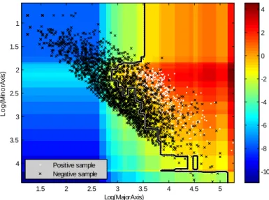
2.2 Detection of rock…sh . . . 40
2.2.1 Boosted detection . . . 44
2.2.2 Shape pre-processing and spurious detection removal . . . 46
2.2.3 Shape-based classi…cation . . . 53
2.3.1 Detection of anomalous areas . . . 62
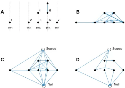
2.3.2 Linking detections . . . 68
2.3.3 Improvement suggestions . . . 73
3 Digital Holographic Instrument Development: Lab to Ocean 74 3.1 Introduction to digital holography . . . 77
3.1.1 Modeling motion during exposure . . . 86
3.1.2 Minimum number of bits . . . 95
3.2 Wigner transform analysis for spherical reference waves . . . 98
3.2.1 Wigner distribution and optical formulation . . . 99
3.2.2 Insights to space-bandwidth limits . . . 101
3.2.3 Space-bandwidth product and sampling volume . . . 108
3.2.4 Depth of …eld . . . 110
3.2.5 Subtle lessons . . . 111
3.3 DH prototype design . . . 112
3.3.1 System components . . . 115
3.3.2 Benchtop systems with oceanic samples . . . 119
3.3.3 Prototype design . . . 122
3.3.4 Power …ltering for Bayer detectors . . . 127
3.3.5 Software for interactive reconstructions . . . 133
3.4 Particle …eld e¤ects . . . 134
3.4.1 Image degradation . . . 150
4 Extracting Information and Images from Holograms 156 4.1 Detection, position estimation, and focus determination . . . 157
4.1.1 Traditional focusing methods . . . 159
4.1.2 Combined focus metrics . . . 169
4.1.3 Metrics using machine learning . . . 174
4.1.4 Object detection from raw holograms . . . 181
4.1.5 Fast depth estimation . . . 192
4.3 Application: Oil droplet size distributions . . . 214
4.3.1 Droplet models . . . 215
4.3.2 Detection using focus metrics . . . 218
4.3.3 Fast circle parameter estimation . . . 222
4.3.4 Droplet classi…cation . . . 228
5 Future Work and Conclusions 235 5.1 Contributions . . . 235
5.2 Applications and extensions . . . 238
5.2.1 Automatic identi…cation of plankton . . . 238
5.2.2 Particle size distributions . . . 239
5.2.3 Biological tracking . . . 240
5.2.4 Digital multiplexing holography . . . 242
5.2.5 Holography on gliders, drifters, and AUVs . . . 246
5.2.6 Riesz-based focus metric . . . 249
Chapter 1
Introduction and Background
Gathering information about biological activity in marine environments has historically been challenging. An immense volume of water, high pressures, mobility, and the range of size scales have all had an impact on our ability to collect data. The oft-quoted metric is that more is known about the surface of the moon than the ocean [329] – because the measurement is that much easier despite the literally astronomical distances.
Tools to meet the challenge of biological and ecological sampling in the ocean have been growing in ability. The original sampling devices, nets and hooks, could return rudimentary information about certain species in a rough area. Their simplicity belied the amount of work required back in the laboratory. Later nets which could include improved spatial information by opening or closing on cue were developed in the late 1800’s and are still used today albeit with electronics to control the spatial sampling [421]. Modern devices which take advantage of electronic sensors and microprocessors are able to shift the burden of observation to the device itself. Instruments which capture data remotely through sound and light have enormously expanded the volume that can be sampled. Given that the ocean is estimated to have 1.3 billion cubic kilometers of water [58] and a sea‡oor larger than 350 million square kilometers, the ability to reach further is especially critical.
An understanding of the biology and ecology of the oceans goes well beyond an acad-emic curiosity. The immediately obvious connection is that the ocean provides food and sustenance for humans and animals alike: in 2008, …sh and seafood provided 15% of the an-imal protein for 3 billion people. Some 90 million metric tons of …sh and aquatic plants are
captured each year, and another 50 million metric tons harvested through aquaculturing. Fishing and aquaculture provide jobs and …nancial support (including dependents) for 540 million people, about 8% of the world population. Fisheries exports were worth a record $102 billion (US dollars) in 2008 [120],[119]. Less obvious is the regulating e¤ect that the ocean has on global temperature and chemistry.
Changes in marine biodiversity “increasingly [impair] the ocean’s capacity to provide food, maintain water quality, and recover from perturbations” [428]. Humans have had a visible impact on worldwide …sh populations, decimating certain populations and signi…-cantly altering the natural balance of many others [304],[34]. Unfortunately, the e¤ect of …sh populations is highly coupled, a¤ecting animals lower in the food chain and modifying the predator-prey balance [430]. Over…shing in particular has been a long-standing prob-lem in human history. Correcting over…shing, when possible, takes decades to centuries to achieve a stable balance [171].
The presence of humans also alters the chemistry of coastal areas through pollution and chemical run-o¤, a¤ecting the marine balance in less direct ways than …shing [171]. Even far from the coasts, changes to the atmosphere are taken up by the ocean as it absorbs carbon dioxide and various anthropogenic chemicals. For example, the ocean is estimated to have absorbed around half of the carbon dioxide released from the combustion of fossil fuels. This has lead to a dramatic reduction in seawater pH and dissolved carbonate, a¤ecting both the plant and animal life that depends on precise acid levels and chemical balances [112],[301].
A number of marine taxa are also sensitive to changes in temperature, leading to ob-servable changes in the biodiversity [382]. Changes in both global and local temperature, both natural and human generated, have the ability to a¤ect these species [143],[346].
Regulatory checks and balances can help preserve the environment and protect the future of the …sheries [34]. The process naturally requires good data about the current state of critical factors and an accurate understanding of how decisions will a¤ect future populations [60],[93]. This is one of the critical areas where ocean sampling and observation enter the picture: obtaining the basic biological and environmental data to inform policy and science.
The interconnectedness of marine ecology means that information is required on multiple scales, and that observations about one species can provide input about another [279],[271]. Plankton, the smallest denizens of the aquatic food chain, are a prime example. Changes to the plankton population can ripple through the entire chain over time [21],[78],[376],[425]. The concentration and health of various plankton can also serve as sensitive indicators for global temperature and various environmental impacts [38],[429],[162],[111]. Tracking these changes generates predictions for the various domains that plankton populations impact – primarily animal, plant, and chemical [154],[22].
1.1
Sampling methods and devices
Gathering the fundamental data about plankton and …sh populations, habitats, and the state of the oceanic environment again returns the discussion to the sampling problem. The ideal sampling instrument would be able to operate over a wide range of biological sizes, discriminate between species, collect data throughout a large volume of water, provide the 3D locations of all the objects in the volume, operate throughout the full ocean depth, and include information about the physical environment (salinity, temperature, currents, particulate matter, chemistry, etc.) – all without disturbing the subjects under study and thus ensuring an accurate measurement. These goals are by no means an exhaustive listing of “ideal”, but provide achievable goals with which to compare the various methods of collecting information in a marine environment. Several of the commonly used instruments for both large scale and planktonic sampling are worth reviewing with these goals in mind.
1.1.1 Large scale measurements
At the largest scale, satellites such as the SeaWiFS1 can provide multispectral information about the upper layer (centimeters to a few meters) of the ocean based on backscattered light. Phytoplankton concentrations (including the ability to discriminated between a few dominant species), chlorophyll content, and size parameters can be correlated to colorimetric measurements [9],[68],[437]. The spatiotemporal coverage of a satellite depends on its orbital
1
track, so that analyses are over relatively long time scales (days to years) and lack precise lateral position information (order of kilometers).
Sound has the ability to travel long distances through water, allowing for long-range sensing and extremely large sampling volumes using sonar. The distance and resolution are coupled to the wavelength so that sonar is reliably capable of imaging large …sh and returning information about biomass [421],[172]. However, to reliably use sonar, models for scattering need to be created and tested. Detecting …sh in the water column is easier than near the bottom where strong re‡ections occur, obscuring the return signal.
Optical solutions provide high resolution and easily interpretable results. Cameras and strobes are regularly mounted onto autonomous underwater vehicles (AUVs) and remotely operated vehicles (ROVs), used by divers, towed behind a vessel, or lowered on cables. They have the ability to image large volumes of water and visually discriminate between …sh species and other centimeter- to meter- sized objects. Capturing information about benthic environments is done regularly. Optical methods are dependent on illumination and low scattering. Obtaining quantitative results from image sets can be time consuming and challenging.
1.1.2 Traditional plankton measurements
The earliest scienti…c device, a plankton or …sh net, sweeps through a volume of water behind a vessel. Nets can sample incredibly large volumes of water. Detailed microscopic analysis of the captured animals provides high speci…city, including information about life stage, gut contents, and reproductive status. Biochemical analyses, including DNA extraction, can also be performed. The three downsides are that spatial information is lost or rough at best, counting the species by hand in the laboratory is laborious and requires the talents of an expert, and the animals are forcibly removed from their environments. Nets which open and close at speci…c depths, for pre-set times, or which respond to signals from a control line (either physical or electronic) improve the spatial speci…city slightly [421],[420].
The Continuous Plankton Recorder (CPR) is a variation of the net-capture-observe philosophy. Instead of collecting plankton using a …xed cod end, water is …ltered past a silk mesh that is slowly transferred between two spools. The position of plankton on the mesh is
combined with knowledge of the CPR’s path to piece together the location. The CPR is also innovative is that it is attached to ships of opportunity as they cross the Atlantic shipping lanes and has been providing data about plankton and micronekton along the transit lines since 1931, one of the longest running experiments in plankton sampling history [298],[412]. E¤orts to automatically analyze plankton captured by CPR-like devices and nets has resulted in the ZooScan system. The captured plankton are laid onto a specialized ‡atbed scanner and imported into a computer where they are recognized using various machine learning approaches. The ZooScan reduces the e¤ort of a human expert in analyzing each planktonic sample [147].
Nets have several problems that makes them unsuitable for certain types of biologi-cals. In particular, fragile objects such as gelatinous animals, trichodesmium colonies, or larvacean houses are destroyed or signi…cantly underestimated [299],[87]. There may also be problems with avoidance, as some motile zooplankton can sense the shear from an ap-proaching net and escape its path [42].
Pumps can increase the water sampled in an area, and are especially useful for studying small-scale relationships. The objects must be immotile, so that pumps are more often used for phytoplankton, microzooplankton, and particulates [289]. Pumps, like nets, have the downside of destroying fragile particulates.
1.1.3 Modern plankton measurements
Sonar, especially high frequency or multi-beam/multi-frequency setups, has seen continued interest for measuring plankton distributions. Euphausiids (krill) and jellies with air voids re‡ect sound with greater e¢ ciency and can be measured to a degree. There has also been work to estimate plankton biomass using sonar. The three biggest problems for sonar are that most plankton is small and soft and thus does not e¢ ciently re‡ect sound, models can only account for general categories of plankton, and the exact sonic properties of the water need to be know to account for changes in the observed signal. The consensus is that sonar may give rough estimates of biomass in certain populations, but is not a suitable tool for determining species or genus, especially for scales less than a millimeter [121],[172],[413],[421].
Non-imaging solutions have also been proposed and used for plankton measurements. The Optical Plankton Counter (OPC) and its later cousin, the Laser Optical Plankton Counter (LOPC) project a light sheet through the water and measure the statistical dis-tribution of light intensities on a set of photodiodes. The OPC/LOPC provides spherical equivalent diameters of objects between about 1.5 mm and 35 mm, thus providing a size spectra only [158],[159],[59]. The Laser In Situ Scattering and Transmissometry (LISST) [3] has also been used to estimate phytoplankton size distributions. Laser light is di¤racted from a small volume and imaged by ring photodetectors. Similar to the OPC/LOPC, the LISST provides size distributions only and is sensitive to the di¤raction pattern [186],[185]. Optical plankton devices have proliferated as cameras and electronics have advanced. The Video Plankton Recorder (VPR), CritterCamR2, Underwater Video Pro…ler (UVP)
[146], and ZOOVIS (and ZOOVIS-SC, for “self-contained”) are all examples of camera-strobe pairs that use direct area imaging. The VPR images microscopic objects with a long working distance and is designed to be towed at high speeds (up to 10 knots for basin-scale measurements). It has a strobe opposite the camera at a slightly oblique angle (a ring in later versions) and essentially captures dark …eld images in either monochrome (original VPR) or color (VPR-II) [85],[84],[86],[88]. The Critter-Cam used Schlieren imaging for phase imaging of microscopic animals with a long working distance [363]. The ZOOVIS instruments use sheet illumination with a thickness on the order of the depth of …eld, and the camera is situated to image side scattering. The ZOOVIS is designed to be lowered downwards so that plankton encounter the light sheet before nearing any mechanical components, reducing avoidance [30],[28],[374].
Line scan camera systems have also been created for imaging plankton. The Shadowed Image Particle Pro…ling Evaluation Recorder (SIPPER) [311],[299] and In Situ Icthyoplank-ton Imaging System (ISIIS) [79] both image objects by recording the shadow projected onto a line scan camera as the device is towed through the water. The SIPPER is intended for smaller plankton while the ISIIS is for larger mesoplankton and nekton. Both systems
de-2
The CritterCamR was developed through a National Geographic Society grant and refers to a ruggedized
video camera that can be used to image animals in their natural habitats. Research using the planktonic
version has been extremely limited since the 1990’s. However, the CritterCamR (or Crittercam) has been
attached to various animals since then, including whale sharks, seals, and various baleen whales – all which have close connections to plankton.
pend on the camera to be towed to generate images and the resulting sample volume (and image distortion) is a function of the tow speed.
Systems for particle imaging include the FlowCytobot [266] and the Submersible Flow-CAM (available commercially from Fluid Imaging Technologies). These pump water through an intake tube into an imaging chamber …tted with microscope optics. Pumps are intended for use with immotile, infrangible particles between a few microns and about half a mil-limeter.
The …nal class of optical measurement devices to discuss here is holographic devices. These occupy an interesting niche between imaging and non-imaging, as the hologram is the di¤raction pattern but is later reconstructed as an image. Notable devices include the a drifting unit from Katz et al., the eHoloCam, a device from Jericho and Kruezer, and the recently released commercial LISST-HOLO. The Katz unit was designed to drift with currents just below the surface, capturing holographic video of plankton interacting within their natural environment [281]. Jericho and Kruezer intentionally image microplankton [179],[137], and there are questions about avoidance that have not been addressed. The devices from Katz and Jericho/Kruezer both appear to be demonstration units and have seen limited use in biological studies. The eHoloCam has potential for biological studies and has been used a limited number of times. Its optical design includes a Q-switched laser, so that the device is best used on powered platforms [366],[367]. Current work with the eHoloCam seems to have stalled since about 2008. Sequoia Scienti…c, the manufacturers of the LISST, released a holographic version of a particle pro…ler in 2010. The engineering is rudimentary but allows basic holographic images to be recorded and reconstructed [321],[253]. A more complete review of holographic devices and their capabilities is included in Section 3.3.
The operating characteristics of the various imaging systems are primarily engineering and implementation choices. For example, the depth range can be extended for each in-strument by using larger housings and syntactic foam. Similarly, power systems and data storage can be modi…ed with enough time, e¤ort, and grant money.
Several excellent papers further review the state of plankton imaging and optical imaging within the ocean, and provide an extended discussion of the exact needs that the devices are attempting to meet [82],[88],[172],[93],[334],[173],[421]. A review paper from Kocak et
al. that discusses new techniques and methods in imaging may be particularly interesting for optical scientists [193].
1.1.4 Combined systems
Each of the individual systems already discussed has its bene…ts and speci…c measurement regimes. Both temporary and permanent combinations have been tried with success for speci…c types of missions. For example, VPRs mounted to AUVs such as JASON, REMUS, or ABE are able to autonomously map out 2D areas or 3D volumes with …ne detail [134], and attempts have been made with ROVs to track zooplankton [302],[317]. Common probes such as conductivity/temperature/density (CTD) sensors and ‡uorometers have been in-corporated into later redesigns such as the VPRII [88] and the ZOOVIS-SC [374]. The BIOMAPPER-II is a particularly wide-reaching system that combines a VPR, CTD, ‡u-orometer, transmissometer, radiometers, cameras, and sonar into a single towed platform [413].
1.1.5 Challenges for microscale optical devices
Direct collection of plankton by nets, CPR, divers, or other similar methods all have the same bottleneck: the need to identify the sample contents. Experts have to painstakingly re-sample and examine the contents. As expected with direct examination, the species resolution is extremely high. Automated or semi-automated systems such as the ZooScan can help reduce the need for an expert but still requires sample preparation and hands-on lab work and have taxonomic resolutions similar to the in situ imaging systems [147]. The rate at which samples can be processed and identi…ed makes nets limited in their coverage and has led to the current sparsity of global data coverage.
Optical devices for plankton are faced with the trade-o¤ between depth of …eld (DOF) and resolution3: the depth is proportional to the square of the resolution (see Chapter 3 and
3Optical resolution is de…ned as the minimum separation in the object plane at which two points can be
discerned as distinct objects [36],[145],[155]. This is a property of both the optical and sampling system. Unfortunately, the “resolution”quoted by a surprising number of authors in the device literature is the pixel size of a detector or the diameter of the smallest isolated point object they can visually observe. Comparisons of resolution and depth of …eld should be taken with a grain of seasalt.
Device Resolution DOF Min. object VPR4 10 50 m (meas.) 0:7 5 cm (meas.) 300 m CritterCamR 15 m (measured) 50 mm (measured) (unknown)
SIPPER > 50 m (pixel size) 96 mm (as reported) 500 m ISIIS > 68 m (pixel size) 20 cm (as reported) 1-2 mm ZOOVIZ 50 m (measured) 1 cm (illumination) 1 mm HoloPOD 6 12 m (meas.) > 250 m per slice 150 m
Table 1.1: Optical sampling capabilities of popular plankton imagers. The resolutions and DOF are quoted as listed in the literature. Measured values for the VPR are based on placing a test object at various locations and judging the useful limits from images captured by the camera. The DOF for the CritterCam was done similarly, using instead a crossed reticle target and visual judgements. The ZOOVIZ DOF was quoted as the thickness of the light sheet illumination. The resolution and DOF of the HoloPOD is based on both theory and measurement, and is discussed in greater detail in Chapter 3. The minimum object size is based on reports from the literature regarding the smallest object that could be reliably identi…ed by the authors.
Figure 3-1 in particular). For example, capturing images with a 50 m lateral resolution results in a DOF of only 2.5 mm. Extremely good resolution also requires a high numerical aperture and thus a minimum lens diameter that grows linearly with the working distance (or, more precisely, with the inverse optical path length, Equation 3.24). The resolution, DOF, and minimum object size for the more popular optical devices which can identify plankton species are listed in Table 1.1, with resolution and depth of …eld as quoted in the literature. These values are considered the working values, determined by experimenting with the actual devices using di¤erent targets. The trend is for resolutions greater than 50 m and limited measured DOFs, so that these instruments are primarily useful for larger plankton. Fast frame rate cameras are used to achieve the necessary sampling volumes. The digital holographic imaging device reported on in this thesis, the HoloPOD, is included as the …nal entry in the table. It was designed with a goal of imaging a large range of plankton sizes, 150 m to 30 mm, with an extended sampling volume per hologram and a volume per unit time comparable to the other optical devices. Chapter 3 reports on the theory, design, and testing of the HoloPOD device.
The optical samplers showcase two other issues that are important for plankton science. The …rst is that the sampling should be quanti…able. The VPR calibrates its sampling volume by measuring point scatterers at locations distributed through the imaging volume
and setting a threshold on a focus metric [318]. The CritterCam does not have a well-de…ned depth range, instead relying on object images to be too defocused or too poorly lit outside the intended sample. The SIPPER and ISIIS systems both require good estimates of the ‡ow velocity to calculate the imaged volume at any instant in time. The ZOOVIZ assumes that the sheet illumination has a sharp spatial cut-o¤ and that objects outside the illumination are not imaged. On the other hand, the HoloPOD has an exact image volume. The second major issue is that of avoidance. Several motile zooplankton and micronekton are able to sense the shear from an approaching device and will attempt to escape, skewing the totals downward. The ZOOVIS and VPR are speci…cally designed to reduce ‡ow e¤ects by using an extended working distance, with ‡uid modeling performed on the VPRII to limit shear in the image volume to levels lower than the detection threshold for most copepods [88]. The SIPPER, on the other hand, funnels its samples through the center of a large duct-like area, potentially leading to signi…cant avoidance. The HoloPOD has a long working distance and a small hydrodynamic footprint, signi…cantly reducing the shear and avoidance concerns.
Quantifying the images captured by optical devices is another signi…cant challenge. Plankton imaging devices have a well-de…ned goal and design, so that the number of meth-ods and software is as numerous as the devices themselves. Examples include AutoDeck and Visual Plankton (VPR/VPRII), Pisces (SIPPER), ZooScan (nets) [147], ZooImage and PhytoImage (FlowCAM), and the Plankton Analysis System and Plankton Interactive Classi…cation Tool (PAS and PICT, general plankton recognition) [246].
1.1.6 Challenges for macroscale optical devices
Cameras mounted on AUVs, ROVs, and carried by divers o¤er a vastly di¤erent set of con-ditions. Variation in the background, orientation, and deforable objects means that experts are often required for parsing the imagery into useful data. Estimating habitat coverage, for example, often involves randomly sampling portions of the imagery and classifying the ob-served points. The totals are then estimated from a small portion of the dataset. Similarly, counting …sh species involves an observer searching through images and tallying the num-bers of the speci…c …sh of interest. Needless to say, this can be incredibly time consuming
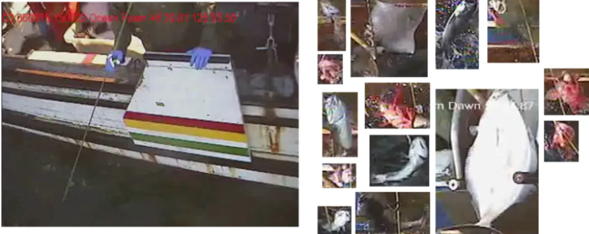
and slow, especially for missions that capture hundreds to thousands of pictures per dive. Addressing the need for automated methods in marine imagery is the goal of Chapter 2. Methods of determining habitat types and detecting rock…sh from a downward looking AUV camera can not only aid a human observer but provide starting points for additional data such as estimating the sizes of …sh or correlating habitat with abundance that would be especially time consuming using standard approaches. Detection and grouping of …sh as they are caught on longlines will also be presented, an above-the-water marine application that has bearing for protecting the …sheries below.
1.2
Contributions and highlights
The main goal of this thesis is to develop and analyze tools for use in detecting and iden-tifying biologically relevant objects in aquatic environments. The majority of the e¤ort is focused on automated methods that are computationally practical for the large datasets generated in oceanography. Good sampling practice is also stressed, with attempts to es-timate and measure the error of various algorithms or predict the performance of a new holographic device for plankton imaging.
The …rst foray is working with traditional images captured by digital cameras. A bag-of-words model is shown to be particularly good at correctly identifying habitats in AUV imagery. Small image patches provide an optimized …lter, and recognition rates are im-proved by computing an independent components analysis on the …lter basis. A multistage detector for rock…sh is created from the same dataset, and includes discussion about why the detector and its features perform as they do. Chapter 2 concludes with detection and grouping of …sh caught during longline operations and recorded by low bandwidth webcams. An improved digital holographic imaging device for use with in situ plankton measure-ments is presented in Chapter 3. Theory predicting how it performs under motion and with limited bit counts informs the engineering decisions. An analysis of the spatial and bandwidth limits of spherical reference holography is done using Wigner transform meth-ods, providing a complete and demonstrably useful model for general in-line holography. The speci…c engineering variables and choices for the digital holographic unit are discussed,
testing performed, and a prototype unit constructed. Real-time software for reconstruct-ing the holographic images is presented. Theory and simulations describreconstruct-ing the e¤ects of particle …elds, such as observed in marine holograms, is discussed.
Computational algorithms for extracting information from holograms captured by the prototype are presented in the fourth chapter. These are especially important for digital holography, limited in widespread use a lack of suitable algorithms for general imaging and descriptions of their performance. Various focus metrics are presented with an emphasis on fast computations for large reconstruction volumes. A novel focus metric that uses local Zernike moments as edge detectors is presented. For holograms which do not require full reconstructions, methods are suggested for quickly estimating the lateral position and depth of objects within holograms. Two approaches are presented for detecting objects laterally, one that extends a summation kernel to spherical reference holography and another that applies local frequency estimates to …nd areas consistent with a holographic signature. A new depth estimator is proposed, based on a normalized spectral response, and is demon-strated to have excellent depth resolution and noise insensitivity. The performance of focus metrics, lateral detectors, and the depth estimator with real-world oceanic holograms is presented. The methods are then applied to locating and sizing oil droplets in the Gulf of Mexico during a recent oil spill.
The …nal chapter discusses a number of extensions and ideas based on the work presented in this thesis.
Chapter 2
Traditional Imaging Methods
Photography is arguably one of the best ways to record information from a distance about our complex world. It has a long list of bene…ts: photography has an incredibly high space-bandwidth product compared to other measurement methods, camera and lens systems are well understood and developed, there is a high degree of ‡exibility in the imaging (for exam-ple, passive or active lighting, di¤erent spectral ranges, color …lters, use of digital sensors, post-processing methods, and temporal information through video), the resulting picture is easy for a human to interpret, and many photographic setups can be inexpensive and simple – all of which contributes to the popularity of photographic methods for both the lay audience and scienti…c studies. The advent of digital cameras and improved computa-tional methods have further boosted the abilities of photography to the point where it is a ubiquitous tool for both science and everyday life.
One of the challenges with modern imaging is that pictures are easy to capture, so that a scienti…c deployment can involve hundreds or thousands of pictures. The burden on an educated observer to quantify the data in those images can be immense – and incredibly time consuming. Computational methods which can reliably replace an observer, or …lter out the important information for an observer, have a number of useful bene…ts: the ability to make complicated measurements (e.g., computing area coverage or fractal dimension), returning results faster than a human, and possible implementation on a vehicle for in situ decisions as a few examples.
oceanic images using image processing and machine learning. Two particular data sources are used as examples: sea‡oor images captured by a downward looking camera on an automated underwater vehicle (AUV), and a low resolution video camera watching …sh on a longline as it is pulled into a boat. These sources di¤er from many others (i.e., tra¢ c and surveillance cameras, product quality control on conveyor belts, or photography in urban environments) in that the relevant information rarely follows a preferential orientation and there is not a straight-forward generative model which describes the varied shapes of the animals in the images. The methods developed in this chapter have application beyond oceanic use, as the purpose is to create texture recognition, object detection, and similarity grouping which has enough ‡exibility to work on the particularly challenging class of aquatic habitats and animals, all valid for cases with more constraints such as man-made textures and objects.
The term “traditional imaging” is used here to denote a detector and lens combination designed to image a plane of the image space onto the sensor –no steps are taken to modify the imaging system for the speci…c task aside from stopping down an aperture or selecting a di¤erent lens. The primary goal is to work with the images created from traditional imaging systems purely from the computational side after capture.
2.1
Habitat classi…cation from textures
Biological information about the sea‡oor is immediately useful for oceanic biologists, chemists, and ecologists [60],[312],[394],[249]. Sea‡oor data has secondary use in the …sheries, as many crustaceans, mollusks, and certain pro…table …sh are benthic during larval stages of their life – if not their entire lives. Information about reef and coral ecology, along with the species inhabiting those areas, can be used as sensitive indicators for changing temperatures and chemical balances in di¤erent parts of the ocean [312],[142],[279],[429].
Habitat discrimination and species identi…cation requires a high level of details and a broad …eld of view. Both tasks bene…t from reliable color information. The SeaBED autonomous underwater vehicle (AUV) is engineered to provide imagery that meets these goals: high quality, a large …eld of view, careful color correction, and a fast enough imaging
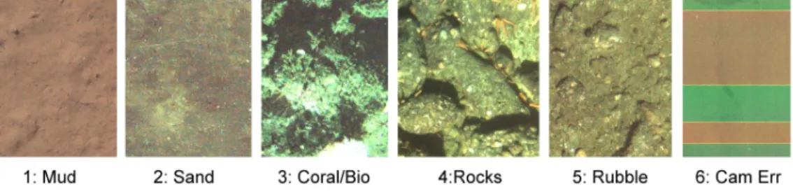
Figure 2-1: Samples of each of the six texture classes evident in the SeaBED images.
rate to acquire continuous swaths of data. During a single deployment, the SeaBED dives to depth, then cruises a few meters above the sea ‡oor capturing several thousand images to an internal storage device [337],[338]. The image are retrieved when the AUV surfaces. Human experts can then analyze the images, searching out animals and interesting features (see, e.g., [384]).
Automated methods for extracting information from sea‡oor data has thus far been lim-ited. The best examples are related to surface topology measurements: three-dimensional topology is made possible with multiple cameras and advanced algorithms for estimating pose and position [284],[283]. Describing the contents of the sea‡oor automatically is a dif-ferent matter entirely. Unsupervised clustering may give computational results, but returns categories which have limited semantic meaning (see, e.g., [52],[285],[353], where multiple clusters correspond to the same category while other environmentally distinct categories are combined into the same cluster). Figure 2-1 shows samples acquired by the SeaBED and illustrates both the subtle visual di¤erences possible (e.g., between mud, sand, and rubble) along with the gross di¤erences (e.g., between mud and coral/bio1) – both reasons why unsupervised learning is perhaps not the appropriate approach for habitat recognition.
The goal of this project is to use machine learning to perform habitat recognition through a texture recognition framework. The example data comes from ten SeaBED dives (Daisy Bank and Coquille Bank o¤ the coast of Oregon and Santa Lucia Bank o¤ the coast of Southern California; see [384] for location maps), a total of around 31,000 images (1.25 MPx color JPEGs, 10 GB total). The images were rigorously color corrected by the SeaBED
1The class label coral/bio denotes rocky areas which have signi…cant biological growth over the surface,
or which have a coral-like appearance due to the biological activity. It does not necessarily indicate a true coral.
team, so that color can be used for classi…cation of species and habitats both. Examples of the …ve predominant habitat classes, along with a sixth class to represent camera errors, are shown in Figure 2-1. The images have a signi…cant range of size and orientations, though there is a bias for upward-facing shadows due to the …xed position of the strobe lights on the AUV. The habitats can also be mixed: sand coats the tops of large rocks or …lls the area between rubble, for example. As mentioned, there is also a …ne line between rocks and rubble and between coral/bio and rocks.
Texture classi…cation has seen a number of new approaches in the past decade [440], including the use of “bag of words”models popularized by Varma and Zisserman [398],[399]. The bag of words (BoW) model compares the statistical distribution of …lter responses for di¤erent textures, much like distinguishing between di¤erent documents by examining the frequency of characteristic word choices2[368]. It is particularly simple in that it disregards the spatial relationships between pixels, so that the …lter response at one pixel is taken to be independent of its neighbor, and thus the distributions of the underlying random …eld need not be estimated. This in turn reduces the possible dictionary space and requires fewer training examples to estimate the distribution space. For natural textures without a preferred orientation (and thus a larger distribution space than oriented textures), this can be especially bene…cial.
This section discusses recognition of sea‡oor textures using bag-of-words models, start-ing initially from the original Varma-Zisserman …lterbank-based techniques and expandstart-ing out to incorporate multiple models per class label. An alternate view of …ltering using image patches is explored, with links to optimal …lter selection and transformation spaces. The resulting methods are tested for their classi…cation accuracy, then used to measure areal habitat coverage across the full dataset –providing results to a problem which would be challenging and extremely time consuming for a human observer, but computationally tractable for a single desktop computer.
2
The bag-of-words model uses many typographic terms based on its lexicographic foundation, the most notable here being a “dictionary”, or codebook, of the most common texture “words”.
2.1.1 Bag of words for texture classi…cation
The bag of words model uses the statistics of an unordered collection of related elements to perform recognition [440],[368]. In the case of texture recognition, those related elements are the texture descriptors computed at each pixel in a digital image, termed “textons” by the computer vision community. A new texture is recognized by …rst determining the best texton to represent each pixel, then comparing the frequency of each texton against its expected frequency for known textures. The term “best” is intentionally vague, as its meaning will change depending on how the similarity between feature vectors is measured3, but is in general a measure of minimum distance.
Training is performed in two steps (Figure 2-2). In the …rst step, a series of …lter responses are computed for each pixel in a set of training images for a single class, forming a feature vector at each pixel. The feature vectors are aggregated and quantized into representative clusters using k -means, with each cluster center representing a texton for that training class. The textons for all training classes are gathered into a dictionary of representative textons.
The second step of training uses the dictionary to estimate texton distribution models for each class. The feature vectors are again computed for each pixel in a training image, then each pixel is labeled with the dictionary texton which has the smallest distance to the feature vector. (If the …lters are normalized to the same value, the response for each feature vector component is on the same order and a Euclidean distance can be used. A weighted Euclidean distance or a Mahalanobis distance, Equation 2.8, may be a better choice if the …lters have di¤erent magnitudes [80],[236].) The frequency distribution of texton labels is then computed and becomes the model for that particular training image. A class model can be estimated by averaging together the models for each training image in that class if the models are similar enough, by using k -means or another clustering algorithm [106] to select a limited number of models if there is dissimilarity between models of the same training class, or by maintaining the entire collection of image models. The …rst two options have
3
One simple example is a feature vector which includes components with di¤erent scales, such as local mean and local entropy. In that case, a Mahalanobis distance [236] may be more appropriate than a Euclidean distance.
Figure 2-2: Steps in VZ texture recognition. In the …rst stage of training, sample images are passed through a set of …lters and their responses clustered to create a set of representative textons for that class. The second stage computes class models based on the frequency of the di¤erent textons appearing in the training images. Classi…cation is done by passing new images through the same …lterbank and computing its distribution of texton responses; the class with the most similar texton distribution is selected as the sample’s label.
the ability to remove or reduce the e¤ect of outliers, while the last option can be sensitive to outliers (which may be desired in some cases) and requires all training images to be labeled correctly.
Recognition of textures is done using a similar method as the second training step. The texton labels are again computed for each pixel of the image of an unknown texture, then the texton distribution is computed. The distribution is compared against the class models and the class with the smallest 2 value is selected as the best estimate. The 2 distance is calculated as 2 =X i (xi yi)2 xi+ yi (2.1)
for two discrete distributions x and y, where xi is the value of the ith bin of x [368].
A number of variations for BoW are immediately obvious: the k -means clustering dur-ing the dictionary creation step can be replaced by a¢ nity propagation [128], k -nearest neighbors [106], or a hierarchical mean shift [278] with the ability to adjust the impor-tance/similarity of individual textons; the 2 distance can be replaced by other distribution-distance measures such as a symmetric Kullback-Leibler [180], Bhattacharyya [4],[33] (which itself is directly related to the Matusita distance [4],[247]), or Kolmogorov-Smirnov metrics; the texton dictionary can be pruned to remove textons appearing in multiple classes; and so on. The interest here is in the overall method, and minor tweaking is left to future users. The remainder of this section will concentrate on using k -means for computationally e¢ cient clustering, a¢ nity propagation when selecting multiple models per class, and 2 for comparing models.
2.1.2 Texture descriptors
The traditional Varma-Zisserman (VZ) approach uses …lter responses to represent a texture description. Their preferred …lter bank is the MR8 bank, which includes eight …lters: three sizes of bar …lters, three sizes of edge …lters, a Gaussian, and a Laplacian of a Gaussian. Each bar and edge …lter is computed for multiple angles and the maximum response across the angles is used as that …lter’s overall response [398]. Other …lter banks are certainly possible; see [398] for descriptions of several types compared in their work. In the exploratory phase
for this work, a …lter bank of scaled and oriented Gabor …lters [198], one using Hu invariants [164], and one composed of local statistics (local mean, local variance, and scaled local entropy) were tried. The …lter bank of local statistics gave reasonable results despite its ad-hoc nature and provides a baseline for comparison. The other …lter banks gave poor results and were not explored further.
Recently, the idea of using image patches extracted directly from the texture images was proposed as a new feature vector. A small block of pixels around the pixel of interest is reshaped into a vector, normalized appropriately, and used directly to create the texton dictionary in the same way as a vector of …lter responses [399]. The texton label assigned to each pixel is then the dictionary texton with the minimum Euclidean distance to that pixel’s image patch.
The patches used here were created by combining grayscale and color information. The image was …rst converted to grayscale, mean subtracted, and normalized to the standard deviation to remove intensity artifacts. Each n n normalized intensity patch was reshaped into an n2 1 vector. Color information was included by appending a 3 1 vector of the mean values of the RGB color channels over the patch, made possible by careful color correction performed during the data acquisition. The RGB values range from [0; 1] ; so that they have similar magnitudes as the normalized intensity information. The use of non-linear color spaces, color invariants [395],[396],[45], or a 3n2 1 vector which retains all of the data from each of the color channels are left for future study. Notably, non-linear color spaces such as HSV or HSL [383] would require a distance metric which incorporates the angular hue component.
The patch approach has several bene…ts. First, it does not require a speci…c …lter bank, removing one level of obfuscation and experimentation. The patch textons may actually be better than arbitrarily selected …lter banks as they are the result of using vector quantization with each texture, forming a compact set of exact representations [140]. Second, patches can act like a kernel method by increasing the dimensionality of the problem, possibly leading to better discrimination [106]. Third, as Varma and Zisserman point out [399], large-scale gradients or textures can be categorized by examining the histograms of the local gradients, so that much of the same information as in …lter banks is present in patches.
Evidence that texton patches contain similar information to …lters can be seen by ex-amining the selected textons. Figure 2-3 shows an example texton dictionary selected for a set of 5 5 patches. A number of patches depict bars, edges, and corners with various ori-entations, similar to the MR8 …lter bank, but with additional speci…city for the scales and spatial frequencies present in the observed data. For comparison, the texton dictionary se-lected by Varma and Zisserman is shown in Figure 2-4, which includes a signi…cant number of man-made textures. The VZ dictionary again contains a large number of bars, edges, and corners, though with a number of high-frequency stripes to accommodate the synthetically manufactured textures. Both of these dictionaries suggest that bars, edges, and corners are good representations of the information content in generic textures. Work from Torralba et al. suggests that this extends to generic images as well: they use a boosting algorithm to select patches (which are used in their work as …lters) which provide good recognition and discrimination between a large number of object categories [385]. Their best …lter patches are shown in Figure 2-5 – and include a number of bar, edge, and corners along with a few more speci…c …lters for classes which are otherwise di¢ cult to discriminate. The overall message is that patches can contain the same information as …lter banks, while o¤ering high speci…city and the ability to generalize.
Dictionary textons are selected in BoW for each class alone, then aggregated together. This has the potential of generating redundant textons. Some dictionaries may also be linearly dependent, since patches span Rn2+3 at most and dictionaries which contain more than n2+ 3 elements are easy to generate. Two transforms to increase the disciminability and independence of the textons were considered: an eigenmode decomposition and an independent components analysis.
The eigenmode decomposition was computed by taking the singular value decomposition (SVD) of a set of dictionary textons. The singular vectors corresponding to non-zero singular values (a total of n2+ 3 at most), termed “eigenpatches”when the SVD is applied to patch textons, are retained as an appropriate basis set for transforming patches into the shared eigenspace. The …rst training stage is modi…ed by projecting the previously-determined dictionary textons into the eigenpatch basis to form a new, transformed dictionary. The second stage is performed by again extracting patches from images, then decomposing the
Figure 2-3: Patch textons selected by k -means for the habitat classi…cation problem. The patches are 5 5 pixels each and there are 30 textons per class for a total of 180 dictionary textons. The textons ‡ow from top to bottom in order of their ordinal class number (Figure 2-1).
Figure 2-4: Dictionary patch textons selected for a collection of man-made textures; …gure is from [399].
Figure 2-5: Patch …lters selected by boosting for recognizing a large class of man-made objects and textures; …gure edited from [385]. Note that the majority of the edges and bars have vertical, horizontal, or 45 degree orientations due to their origin from man-made objects –which is di¤erent from unoriented natural objects.
patches into the eigenpatch basis to form transformed feature vectors. These eigenpatch vectors are used with the transformed dictionary to create the class models. The recogni-tion step similarly includes an eigenpatch transformarecogni-tion when computing models for the unknown texture.
An example set of eigenpatches corresponding to the patches in Figure 2-3 is depicted in Figure 2-6. (Colors may be inverted since the singular vectors have a sign ambiguity.) The …rst few eigenpatches depict bars and edges, similar to Figures 2-3, 2-4, and 2-5 and the MR8 …lter bank – these are the basic building blocks which form the basis of many images. Higher spatial frequencies are reserved exclusively for the eigenpatches correspond-ing to the eigenvalues with smaller magnitude (higher indices). However, a signi…cant amount of energy is spread into the higher-index eigenpatches (20% of the energy is in the last 14 of 28 patches), indicating that there may be useful discriminability in the higher eigenpatches. The problem is that these higher-index eigenpatches individually have small energy compared to the common low-index eigenpatches, making the di¤erence between the transformed patches di¢ cult to detect.
The second transformation attempts to …nd a more discriminable basis set by using an independent components analysis (ICA). The ICA …nds a basis in which the data are less Gaussian and are thus closer to being statistically independent [170]. The resulting “ICA
E ig 1 E ig 2 E ig 3 E ig 4 E ig 5 E ig 6
E ig 7 E ig 8 E ig 9 E ig 10 E ig 11 E ig 12
E ig 13 E ig 14 E ig 15 E ig 16 E ig 17 E ig 18
E ig 19 E ig 20 E ig 21 E ig 22 E ig 23 E ig 24
E ig 25 E ig 26 E ig 27 E ig 28
Figure 2-6: Eigenpatches for a set of 5 5 patches. A total of 28 patches are available here due to the additional three color components. Eigenpatches have been normalized for dis-play, and colors may be inverted. The patches are formed by reshaping the intensity portion of the singular vector and applying multiplying by the mean “color”. The eigenpatches are shown in decreasing order of how much signal energy they represent.
patches” are, in one sense, more unique and thus give better discriminability. Figure 2-7 shows the ICA patches generated from the forward ICA transform4 corresponding to the patch dictionary of Figure 2-3 [169],[138]. (Color may be inverted; similar to eigenpatches, the ICA transform vectors do not include sign information.) The ICA patches tend to highlight small peaks or dips and, perhaps more importantly, where those peaks and dips appear in the patch: the shifts, such as between ICA patches 2, 4, and 8, di¤er in Fourier space by their phase ramps. (Similarly, consider ICA patches 10, 14, and 22). This suggests that the ICA patches are types of phase-space …lters. The ICA patches are used like the eigenpatches, transforming image patches during the model generation stage of training and recognition.
4
An ICA includes both a forward and inverse transform. The forward transform describes the underlying components which are used to generate the observed features, while the inverse maps observations back to the independent feature space. This is comparable to the U and V matrices of the SVD, where a matrix A
IC A 1 IC A 2 IC A 3 IC A 4 IC A 5 IC A 6
IC A 7 IC A 8 IC A 9 IC A 10 IC A 11 IC A 12
IC A 13 IC A 14 IC A 15 IC A 16 IC A 17 IC A 18
IC A 19 IC A 20 IC A 21 IC A 22 IC A 23 IC A 24
IC A 25 IC A 26 IC A 27 IC A 28
Figure 2-7: ICA patches computed for 5 5 pixel image patches; shown here are the forward ICA transforms.
2.1.3 Multiple models per class
Natural textures are particularly prone to have greater variation within each semantic class. For example, the di¤erence between small boulders and large rubble is visually apparent, leading to distinct models for each component – but both have the same connotation for a biologist since they support the same set of species. There are also a number of images where the di¤erence between rubble and small boulders is minor (or some rubble exists with a set of small boulders and vice versa), so that consistently labeling the images cleanly into two separate classes is di¢ cult at best. The best solution for this case would be to include multiple models, at least one for small boulders and one for rubble, under the same rocky label.
There are two ways of creating multiple models per class. One is to retain a model for every image in the training set. This has the ability to map out a large feature space, assuming each of the training images has the correct label. Unfortunately, this approach can be sensitive to outliers, especially if models from one class overlap into the area of another class. Another issue is that many more training samples are required to adequately map out the feature space belonging to each class. Clustering models together can help alleviate
some of these issues: it reduces the e¤ects of outliers and can select reasonable models with fewer samples. A caution with clustering is that it reduces the speci…city of the feature space-to-class mapping. In this work, clustering was used to choose a limited number of relevant models for each class so that a smaller number of training samples could be used. Clustering, or unsupervised learning, has a huge proliferation of methods. Already, k -means was discussed as a simple way of selecting speci…c numbers of clusters – if the number of clusters is known a priori. Besides needing to know the number of clusters, it has a potentially serious drawback: the cluster centers are taken as the mean of the cluster elements, so that cluster centers may not actually be members of the set (especially if the wrong number of clusters are used).
A¢ nity propagation (AP) is a new method which uses the similarity between elements to select a few elements which best exemplify the cluster characteristics. It has been shown to select better clusters than k -means in several cases, can better accommodate clusters with varied sizes, and can cluster based on non-standard similarity metrics [128],[252]. One of the reasons that AP is used in this work is that the clustering algorithm returns a measure of the net similarity of the clusters, N S(p); and the number of clusters, C(p); as a function of the initial clustering preferability, p: An AIC-like criterion [46],[7] is computed as
AIC0 = 2C (p) 2N S (p) ;
and the model clusters corresponding to the minimum AIC0 are selected as the appropriate models for the training class. The original derivation from Akaike includes a logarithm of the likelihood function [7], which is replaced by N S here as a way to approximately measure the agreement of the data with the clustering. The scale value of two was selected exper-imentally to give reasonable clustering results. The similarity between clustering elements was computed using the 2 distance. Most training classes in the habitat data set resulted
2.1.4 Classi…cation accuracy
The real-world sea‡oor habitats of Figure 2-1 from the SeaBED AUV dataset were tested for classi…cation accuracy using statistical …lters5, direct image patches, eigenpatches, and
ICA patches. A total of 631 images with uniform class membership, as judged by a human expert, were selected randomly from the over 30,000 images in the example dataset and labeled with one of mud, sand, coral/bio, rock, rubble, or camera-error as the true class label. Representative textons were found by randomly selecting 10,000 textons from each class and using k -means to compute k cluster centers; the k clusters were aggregated from each class to form a complete dictionary with a total of 6k texton elements. Patch transforms were applied to the entire dictionary. Methods which used a single model per class formed the model from the 10,000 textons used to initially form the dictionary since they represented a random selection drawn throughout the class. The multiple models per class case used twenty images randomly selected from each class to form an initial set of models. The texton frequencies were computed for each of the twenty images and a¢ nity propagation used to select appropriate class models. Images corresponding to the models selected to represent the class were removed from the test set. The confusion matrix and true positive rate were recorded for each experiment. Throughout this sub-section, k is the number of textons per class used when creating the dictionary, n is the number of pixels per edge in an image patch (i.e., the patch is sized n n), a “-S” following a method name denotes that the results were computed using a single model per class (e.g., “Eigenpatches-S”) and a “-M” denotes the use of multiple models per class.
Overall classi…cation rates for the ad-hoc collection of statistical …lters (local mean, local standard deviation, and scaled local entropy) is shown in Table 2.1. The statistical …lters gave better performance than either the MR8 or Gabor …lter banks despite its contrived nature. The table is shown for the sake of providing a baseline: for the SeaBED images, overall recognition rates of 85-89% are possible with the right set of …lters. (Gabor and MR8 were in the 65% to 80% range.) The goal for patch methods is then to improve the
5
Additional testing with MR8 and Gabor …lter banks was done, but is not reported here: the results were poor and not particularly illuminating. The statistical …lters themselves are reported here for the sake of providing a baseline.
k Filter-S Filter-M
10 85.9% 86.7%
30 89.1% 84.6%
Table 2.1: True positive results obtained using statistical …lters.
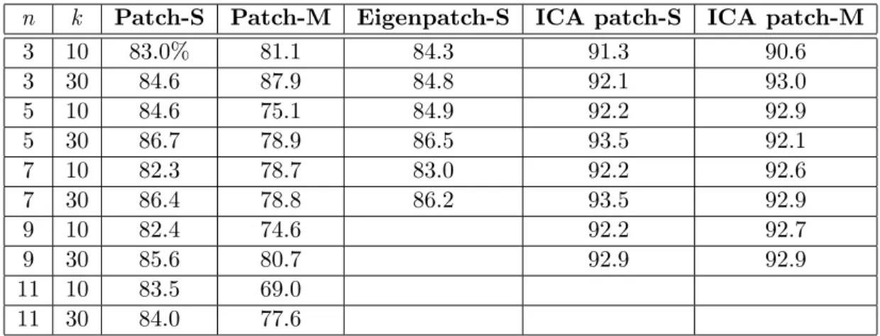
n k Patch-S Patch-M Eigenpatch-S ICA patch-S ICA patch-M
3 10 83.0% 81.1 84.3 91.3 90.6 3 30 84.6 87.9 84.8 92.1 93.0 5 10 84.6 75.1 84.9 92.2 92.9 5 30 86.7 78.9 86.5 93.5 92.1 7 10 82.3 78.7 83.0 92.2 92.6 7 30 86.4 78.8 86.2 93.5 92.9 9 10 82.4 74.6 92.2 92.7 9 30 85.6 80.7 92.9 92.9 11 10 83.5 69.0 11 30 84.0 77.6
Table 2.2: Recognition results for various patch-based methods. Values are the overall true positive rates.
recognition rates signi…cantly over the rates from …lter methods.
A selection of results for patches are shown in Table 2.2 (additional experiments with larger n and additional patch-based methods, such as MRFs, such as in [399], is not shown here). The direct use of patches, Patch-S, has comparable results to the statistical …lters and better results than the MR8 …lter bank, supporting the idea that patches have enough representational power to rival …lters. This in itself is useful as it reduces the work required by an expert in …nding and selecting a speci…c …lter bank. Patches with multiple models have signi…cantly worse performance due to confusion between the coral/bio, rock, and rubble classes. These classes would have had at least one model close to a model from the other classes, a drawback of having too many models to span a small feature space. The use of eigenpatches did not signi…cantly increase the discriminability above that of direct patches. ICA patches, both single and multiple model, increased the recognition rates markedly, by 6-10% over direct patches. The statistical independence generated by the ICA transform appears to boost the discriminability and is worth the additional computational e¤ort in computing the ICA (a slow process for high-dimensional data but done only once during training) and applying the transform to each patch.
Statistic Patch-S Patch-M Eigenpatch-S ICA patch-S ICA patch-M
Mean TP Rate 84.4% 78.2 85.0 92.7 92.7
Std. Dev. 1.48% 4.92 1.28 0.69 0.76
Best (n; k) 86.7% (5,30) 87.9 (3,30) 86.5 (5,30) 93.7 (5,60) (7,60) 94.8 (9,60)
Total Number 16 10 6 24 24
Table 2.3: Statistical summary of experiments with patch-based methods. Mean, standard deviation, and best recognition rate are percentages.
Mud Sand Coral/Bio Rock Rubble Error TP Rate
Mud 97 100% Sand 3 272 3 97.8% Coral/Bio 26 2 2 86.7% Rock 2 3 101 11 86.3% Rubble 1 2 85 96.6% Error 2 1 0 18 85.7%
Table 2.4: Confusion matrix for the best classi…er found during experimentation. The true class is listed in the rows, the estimated class in the columns. Zeros are left blank for clarity of comparison.
The mean classi…cation rate across all (n; k) combinations is shown in Table 2.3 for each method. The statistics assume that the major contribution is from the method as opposed to the patch size or dictionary size and provide rudimentary evidence that the ICA patches are indeed better than the other patch methods. For the direct patch, sizes of up to n = 11 were used for a total of sixteen experiments. For the ICA patches, a total of 24 experiments were tried with dictionaries ranging from ten to sixty textons per class in steps of ten.
The confusion matrix corresponding to the best recognition rate over all the experiments, 94.8% overall true positive, is shown in Table 2.4. The confusion matrix corresponds to ICA patches-M with n = 9 and k = 60: The greatest source of confusion is between coral/bio, rocks, and rubble –all of which have a similar visual appearance. In particular, the di¤erence between small rocks and large rubble is a matter of opinion, so that the classi…er error may not have a major impact on the …nal biological understanding.
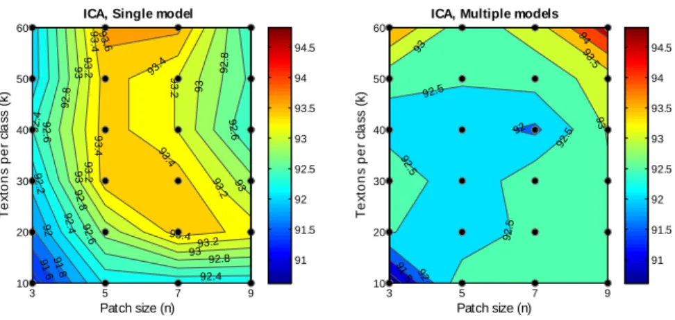
The ICA patches showed markedly better recognition rates over …lters, direct patches, and eigenpatches. Examining the results as a function of n and k; shown for both single and multiple models per class in Figure 2-8, indicates that the high rates are not statistical ‡ukes but vary smoothly with the parameters. The variation across the parameter space
![Figure 2-4: Dictionary patch textons selected for a collection of man-made textures; …gure is from [399].](https://thumb-eu.123doks.com/thumbv2/123doknet/14436357.516086/31.918.273.644.645.935/figure-dictionary-patch-textons-selected-collection-textures-gure.webp)