A Benchmark for Rough Sketch Cleanup

HAL Id: hal-02939477

https://hal.archives-ouvertes.fr/hal-02939477

Submitted on 30 Sep 2020

HAL is a multi-disciplinary open access

archive for the deposit and dissemination of

sci-entific research documents, whether they are

pub-lished or not. The documents may come from

teaching and research institutions in France or

abroad, or from public or private research centers.

L’archive ouverte pluridisciplinaire HAL, est

destinée au dépôt et à la diffusion de documents

scientifiques de niveau recherche, publiés ou non,

émanant des établissements d’enseignement et de

recherche français ou étrangers, des laboratoires

publics ou privés.

A Benchmark for Rough Sketch Cleanup

Chuan Yan, David Vanderhaeghe, Yotam Gingold

To cite this version:

Chuan Yan, David Vanderhaeghe, Yotam Gingold.

A Benchmark for Rough Sketch Cleanup.

ACM Transactions on Graphics, Association for Computing Machinery, 2020, 39 (6), pp.163.

�10.1145/3414685.3417784�. �hal-02939477�

A Benchmark for Rough Sketch Cleanup

CHUAN YAN,

DAVID VANDERHAEGHE,

YOTAM GINGOLD,

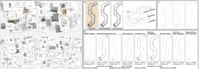
vectorized shape strokes shading scaffold thresholded original disance: running-time:0.00459277 Poly Vector → Stroke Aggregator disance: running-time:0.00403103 Topology Driven→ Stroke Aggregator b) c) a) d) [Favreau et al. 2016] disance: running-time:0.0031155 Fidelity Simplicity

[Simo-Serra et al. 2018a] disance: running-time:0.003455 Mastering Sketching

[Bessmeltsev and Solomon 2019] disance: running-time:0.0025350 Poly Vector [Liu et al. 2018] disance: running-time:0.00427793 Stroke Aggregator [Noris et al. 2013] disance: running-time:0.0032115 Topology Driven [Parakkat et al.. 2018] disance: running-time:0.003571 Delaunay Triangulation [Simo-Serra et al. 2018b] disance: running-time:0.003912 Real-Time Inking

Fig. 1. Our dataset consists of rough sketches (a, top) collected from the wild along with redundantly cleaned versions by professionals (a, bottom). Each sketch is manually vectorized into shape and auxiliary layers (b) and professionally cleaned by multiple artists to create a ground truth (c). We use our dataset to evaluate state-of-the-art rough sketch cleanup algorithms and identify open problems (d). Pipe image © Patrick Murphy CC-BY-2.0.

Sketching is a foundational step in the design process. Decades of sketch processing research have produced algorithms for 3D shape interpretation, beautification, animation generation, colorization, etc. However, there is a mismatch between sketches created in the wild and the clean, sketch-like input required by these algorithms, preventing their adoption in practice. The recent flurry of sketch vectorization, simplification, and cleanup algo-rithms could be used to bridge this gap. However, they differ wildly in the assumptions they make on the input and output sketches. We present the first benchmark to evaluate and focus sketch cleanup research. Our dataset consists of 281 sketches obtained in the wild and a curated subset of 101 sketches. For this curated subset along with 40 sketches from previous work, we commissioned manual vectorizations and multiple ground truth cleaned versions by professional artists. The sketches span artistic and technical categories and were created by a variety of artists with different styles. Most sketches have Creative Commons licenses; the rest permit academic use. Our benchmark’s metrics measure the similarity of automatically cleaned rough sketches to artist-created ground truth; the ambiguity and messiness of rough sketches; and low-level properties of the output parameterized curves.

Authors’ addresses: Chuan Yan, [email protected], George Mason University; David Vanderhaeghe, [email protected], IRIT CNRS Université de Toulouse; Yotam Gingold, George Mason University, [email protected].

Permission to make digital or hard copies of all or part of this work for personal or classroom use is granted without fee provided that copies are not made or distributed for profit or commercial advantage and that copies bear this notice and the full citation on the first page. Copyrights for components of this work owned by others than the author(s) must be honored. Abstracting with credit is permitted. To copy otherwise, or republish, to post on servers or to redistribute to lists, requires prior specific permission and/or a fee. Request permissions from [email protected].

© 2020 Copyright held by the owner/author(s). Publication rights licensed to ACM. 0730-0301/2020/12-ART163 $15.00

https://doi.org/10.1145/3414685.3417784

Our evaluation identifies shortcomings among state-of-the-art cleanup algo-rithms and discusses open problems for future research.

CCS Concepts:• Computing methodologies → Image processing; Graphics systems and interfaces; Shape analysis; • Applied comput-ing → Computer-aided design.

Additional Key Words and Phrases:sketch, drawing, design, cleanup, beautification, dataset, benchmark

ACM Reference Format:

Chuan Yan, David Vanderhaeghe, and Yotam Gingold. 2020. A Benchmark for Rough Sketch Cleanup. ACM Trans. Graph. 39, 6, Article 163 (December 2020), 14 pages. https://doi.org/10.1145/3414685.3417784

1 INTRODUCTION

Sketching is a foundational step in the design process. The design funnel [Kriebel 2017; Newman 2002] begins with broad latitude for idea generation. As the funnel narrows, ideas are refined and evaluated, until a finished artifact emerges. Sketches can be created quickly and inexpensively, but play only an indirect, inspirational role in later design stages of the design process. In contrast, the later stages are time-consuming, tedious, and costly.

Decades of research into sketch processing have produced a large literature of algorithms for tasks such as 3D inference [Andre and Saito 2011; Bessmeltsev et al. 2015; Kaplan and Cohen 2006; Lipson and Shpitalni 1996; Shao et al. 2012, 2013; Shtof et al. 2013; Xu et al. 2014; Zheng et al. 2016], UI design [Landay and Myers 1995], and in-between animation [Whited et al. 2010; Yang et al. 2018]. These research works remain underused in practice since they typically

expect clean, sketch-like input rather than the rough, messy sketches found in the wild.

Algorithms for vectorization, rough sketch cleanup, and simpli-fication have the potential to bridge this gap, by vectorizing and cleaning rough sketches for further algorithmic processing. Such algorithms have been explored in the past [Barla et al. 2005; Or-bay and Kara 2011]. In the last five years, there has been a flurry of work [Bessmeltsev and Solomon 2019; Favreau et al. 2016; Liu et al. 2018, 2015; Noris et al. 2013; Parakkat et al. 2018; Simo-Serra et al. 2018a,b]. These works differ substantially in the assumptions they make on the input and output sketches. Some take vectorized input (parametric curves), some take raster input with clean back-grounds, and some take raster input with no explicit restrictions on the background e.g. paper texture. Most output parametric curves, some output in raster form. Most do not consider shading or texture strokes. As ground truth cleaned sketches are unavailable, each approach demonstrates its output on a small set of ad-hoc

exam-ples.1This presents two problems: (1) The examples do not reflect

the variety of rough sketches found in the wild; and (2) comparing approaches is difficult without a common dataset.

Contributions. We introduce a benchmark for rough sketch clean-up, with the goal of bridging the gap between sketches in the wild and sketch-processing algorithms (Figure 1):

• A collection of 281 sketches gathered from the wild. The sketches cover a diverse set of intended uses and styles. The vast majority of rough sketches have Creative Commons li-censes allowing derivative works and commercial uses; the remaining 18 sketches come with explicit permission for aca-demic use.

• A curated subset of 101 sketches along with 40 sketches from previous work which we professionally vectorized and cleaned. The cleaned sketches form a ground truth for sketch cleanup. Each sketch was cleaned by 3–5 artists. The curated sketches have a balanced distribution of uses and styles. We professionally vectorized the rough sketches for algorithms which require vectorized input. We commissioned a total of 526 professional derivative works (vectorizations and clean-ings).

• Computational metrics for evaluating sketch cleanup algo-rithms and analyzing properties of our dataset. Our met-rics evaluate the similarity of automatically cleaned rough sketches to artist-created ground truth; the ambiguity and messiness of rough sketches; and low-level properties of the output parameterized curves.

• An analysis of the cleanup performance of seven recent al-gorithms and two pipelines composed of a vectorization fol-lowed by a cleanup algorithm.

• A clear problem statement that identifies desiderata for down-stream applications, characteristics of sketches found in the wild, and open challenges.

1_{See Figures 4, 7, and 8 for examples from StrokeAggregator [Liu et al. 2018] marked}

©Enrique Rosales. See Figure 10 for examples from Favreau et al. [2016]. See Figure 15 (a,f) for examples from Liu et al. [2015]. Additional examples can be seen in the supplemental materials.

Our benchmark assesses the state of algorithmic sketch cleanup, provides directions for future research, and will directly benefit data-driven cleanup algorithms. Future algorithms capable of clean-ing our benchmark may bridge the gap between real-world design processes and decades of sketch-processing algorithms.

2 RELATED WORK

Rough sketch cleanup/line drawing simplification. Barla et al. [2005] were the first to present an algorithm for line drawing simplification, in which a complex, vector graphic drawing is “redrawn” with fewer strokes. They do this by clustering strokes and then replacing each cluster with a single representative curve. Numerous later works have been proposed following this same basic cluster-and-replace framework for vector graphics [Liu et al. 2018, 2015, 2019; Ogawa et al. 2016; Orbay and Kara 2011; Shesh and Chen 2008]. Another line of work simultaneously vectorizes and simplifies a raster image of a sketch [Bessmeltsev and Solomon 2019; Donati et al. 2019; Favreau et al. 2016; Kim et al. 2018; Noris et al. 2013; Parakkat et al. 2018]. This is a more challenging problem, as parametric data is unavailable for the input curves. Recently, Simo-Serra et al. introduced a series of data-driven rough sketch cleanup approaches using convolutional neural networks [Simo-Serra et al. 2018a,b, 2016]. Unlike the other approaches, Simo-Serra et al.’s work outputs a raster sketch rather than a parametric vector graphic. This area has received substantial interest in recent years; 12 of 16 of these works were published in the last five years.

Datasets. The data-driven approaches by Simo-Serra et al. [2018a; 2018b; 2016] use a dataset that was created in reverse: artists created rough sketches for existing clean sketches. This approach does not capture rough sketches found in the wild, particularly the ambigu-ity that can exist and lead to differing clean interpretations. This dataset is purely raster-based, yet downstream sketch-processing algorithms require parametric curves (vector graphics). In contrast, our dataset was created in the natural direction, by cleaning rough sketches found in the wild. Our dataset is also available as vector graphics.

The OpenSketch dataset [Gryaditskaya et al. 2019] contains prod-uct design sketches of 12 carefully chosen objects drawn in a con-trolled environment in order to capture parametric strokes with time accuracy. The drawings are all rough, not clean. We did not include them as rough sketches in our dataset, because they were created in “domesticated” conditions. Our dataset is composed of sketches in the wild—drawn in uncontrolled environments—in order to capture the diversity of real-world practice.

The QuickDraw [Ha and Eck 2018], Eitz et al. [2012], and Sangkloy et al. [2016] datasets contain a large quantity of novice sketches. Since they are drawn by novices, the sketches do not reflect the complexity of sketches that many sketch-based algorithms intend to process. The vast majority of sketches in our dataset were drawn by skilled artists. The Manga109 [Matsui et al. 2017] and Danbooru [Branwen 2019] datasets contain a large quantity of professional and amateur manga-style drawings. The drawings are polished, unlike the rough sketches in our dataset. Moreover, none of these datasets contain pairs of rough and cleaned sketches.

Beautification. Algorithmic beautification applies aesthetic ideals to an existing drawing. Pavlidis and Van Wyk [1985] introduced this problem statement and an algorithm for beautifying figures as a post-process. The idea of improving a geometric model with aesthetic constraints dates back to Sketchpad [Sutherland 1963]. Several approaches proposed to create clean hand-drawn sketches by beautifying rough strokes on the fly during drawing [Bae et al. 2008; Fišer et al. 2016; Frisken 2008; Grimm and Joshi 2012; Igarashi et al. 1998]. These approaches require artists to change their tools. They cannot be applied as a post-process to an existing sketch. In contrast, we focus on rough sketch cleanup as a post-process that allows artists to continue drawing with their preferred tools. Beautification of higher-level goals, such as straight lines, parallel or perpendicular angles, and even spacing, may result in global changes to a drawing and are out of scope for rough-sketch cleanup. High-level beautification is a potential downstream sketch processing application for cleaned sketches.

3 MOTIVATION

The motivation for our benchmark is to bridge the gap between sketches created in the wild and input requirements for sketch processing algorithms. Downstream sketch processing algorithms include activities as straightforward as filling regions with color and as complex as inferring 3D geometry. We design our problem statement around this purpose. Unlike the “domestic” examples often used in previous work, sketches in the wild are ecologically valid. They were created by artists for their own needs and reflect artists’ natural tools, environments, and purposes. This avoids many sources of bias present when data is created or commissioned with the intention of being suitable for an algorithm. As a result, they can be used to cross-validate sketch processing algorithms.

Many recently proposed algorithms are relevant to this problem, despite having differently stated goals. These algorithms variously categorize themselves as vectorization (converting a raster image into a vector representation, with complexity stemming from han-dling ambiguities in the raster data), simplification (“in which a smaller set of lines is created to represent the geometry of the origi-nal lines” [Barla et al. 2005]), and cleanup or consolidation (cluster-ing raw strokes into aggregate curves). A researcher or practitioner is likely to consider any of these approaches when seeking to solve the bridging problem.

Downstream sketch processing algorithms typically expect sketch-like input in the form of clean, parametric curves rather than raster images. Curves should meet precisely at junctions. Regions should be watertight. A continuous curve should not be stored as multi-ple independent, shorter curves. See, for exammulti-ple, Figure 2. These properties are often assumed by downstream sketch processing applications, or else they spend considerable effort relaxing this as-sumption. 2D-to-3D lifting algorithms often assume that continuity and junctions in the 2D artwork imply continuity and junctions in the 3D shape [Andre and Saito 2011; Bessmeltsev et al. 2015; Kaplan and Cohen 2006; Lipson and Shpitalni 1996; Xu et al. 2014; Zheng et al. 2016]. In-betweening algorithms similarly assume that continuity and junctions should be preserved during interpolation [Whited et al. 2010; Yang et al. 2018]. Filling a region with color may

scaffold lines global _tilt paper texture redundant, loose and messy shading texture ambiguous without global context global asymmetry Rough Cleane d

Fig. 2. Top: Example rough sketches in the wild. Sketches in the wild are typically raster and contain redundant, loose, and messy strokes; strokes which are not part of the shape of the object (e.g. shading, scaffold, tex-ture); strokes which are ambiguous without global context; strokes varying thickness and weight; paper texture; and global inaccuracies. Bottom: Pro-fessionally cleaned sketches serve as ground truth for our dataset. Shape strokes only are shown. Cleanup does not include correcting inaccuracies with global effect, such as the tilted minarets or asymmetric domes. Animal image ©AP CC-BY-SA-3.0, royal palace image ©Jinho Jung CC-BY-SA-2.0.

require watertightness, particularly if the boundary of the region is composed of multiple disconnected curves.

3.1 Characteristics of sketches in the wild

Various characteristics of sketches in the wild distinguish them from more straightforward or idealized examples often considered in the literature. As shown in our evaluation (Section 5), these characteristics present challenges and remain open problems for rough sketch cleanup algorithms. See Figure 2 for illustrations.

Raster Format. Rough sketches in the wild are often stored in raster form. Based on our experience collecting our dataset (Sec-tion 4 File Formats) and a survey of 56 artists, designers more fre-quently draw using raster-based software or scan their work from the physical world. Ambiguities arise from repeated strokes, gaps, and short overlapping strokes. Strokes often over- or undershoot junctions. These ambiguities are exacerbated in raster input. When scanned from the physical world, paper texture and environmental lighting may be visible. See Figure 2 for labeled examples of rough and cleaned sketches.

Varying thickness and weight. Artists often draw strokes with varying thickness and weight. This is deliberate and contributes to the aesthetic appeal of a sketch. Cleanup algorithms should consider or preserve such properties, though it is rare that they do. (Barla et al. [2005] is a notable exception.)

Non-shape strokes. Several kinds of non-shape strokes or marks appear in sketches in the wild:

• Shaded regions (which could be solid regions of color or hatched) frequently occur. Shading can provide information about lighting or surface normals.

• Texture is sometimes drawn, like stone or grass.

• Scaffold strokes or construction lines which are intermediate strokes created to aid in drawing the final shape strokes. Scaf-fold lines depict regular shapes (such as straight, parallel lines or axis-aligned boxes) that can serve as global beautification cues.

• Text annotations sometimes appear. We manually removed text annotations from our dataset.

These are typically not expected by downstream algorithms. See Figures 1–3 for examples from our dataset.

Physical artifacts. Paper texture and environmental lighting may be present. This is often considered a separate pre-processing step for algorothmic sketch clean-up. More attention should be paid to this step. It is critical to robustly ignore them. Rough sketches virtually always come in raster form (all of our dataset), either scanned from the physical world (34% and 39% of our full and curated datasets, respectively) or drawn in a raster graphics program (the remainder). It strongly influences the quality of algorithmic cleanup. Global context. Correctly interpreting a stroke in one part of a shape may require global context. This is the case for a stroke which is the continuation of a partially occluded stroke. This is also the case for a stroke which has two local interpretations but clearly forms part of a perceptual whole, such as the bottom hem of the shirt in Figure 2.

Deliberately non-smooth strokes. How much smoothing or straight-ening should be applied to deliberately messy strokes? In some architectural sketches in our dataset (e.g. Figure 2), the strokes have a deliberately shaky appearance.

3.2 Problem Statement

We seek an algorithmic solution to rough sketch cleanup, in which a sketch from the wild (in raster or vector format) is converted into a neatened parametric vector graphics representation:

• Strokes that are loose and messy should be consolidated into a single clean stroke. Redundant and errant strokes should be removed.

• Strokes should meet precisely at junctions.

• Stroke thickness and color should be close to the original sketch.

• Decorative strokes, such as shading and texture, should be identified and treated separately.

• Scaffold or construction lines should be identified, separated, and themselves cleaned.

• Cleanup should not add detail not present in the original sketch or replace, for example, a hat in the input with a more fashionable one (Figure 4). Every stroke in the output should be a cleaner or neater version of strokes present in the input.

Due to ambiguities in a rough sketch, global context and high-level perception may be required to correctly interpret a rough stroke. However, rough sketch cleanup does not include operations with global effect, like correcting inaccurate perspective, imperfect ellipses, or adjusting the overall angle of a shape such as a leaning tall building. Even small changes with global effect may require warping the entire sketch.

Rough sketch cleanup can be easily performed by humans with a few caveats. Ambiguous regions in a sketch will lead to inconsistent cleanup. It is difficult for humans to create junctions with perfect as opposed to visual precision. It is difficult for humans to match stroke thickness and color.

4 DATASET

To evaluate and focus research into rough sketch cleanup, we gath-ered a dataset of rough sketches obtained in the wild. Our dataset consists of 281 sketches, from which we curated a subset of 101 sketches with a more even distribution of genre, style, and artist. The curated subset is also a trade-off reflecting the manual effort in-volved in ground truth creation. To curate the set, we independently marked at most five sketches per artist to “definitely” include in the subset and an unlimited number of additional sketches to include “if needed.” By marking no more than five sketches per artist, we prevented any artist from dominating their genre. Sketches deemed less suitable were left unmarked. The curated subset consists of those images which the majority marked as “definitely” and the others marked as “if needed.”

4.1 Sketch Collection

We collected sketches by searching publicly available online sources (e.g. Flickr, DeviantArt, forums, blogs, artist web pages) for Creative Commons artwork, via direct outreach to personal and professional contacts and indirect outreach by asking our contacts to distribute a link to an online submission form, by scanning a book for which we could obtain suitable permission, and by paying artists on UpWork to license some of their existing drawings under a Creative Com-mons license. We sought sketches that were primarily line drawings, not colorful or shaded. (We found it impossible to avoid shading entirely, particularly among design sketches.) We sought sketches that exhibited some amount of roughness. We sought sketches, not novice doodles, reflecting some amount of expertise gained by delib-erate practice. We provide a web interface for browsing and filtering these sketches in our supplemental materials.

We also collected ground truth data for 40 sketches used in previ-ous work. We do not count these 40 in our dataset, as they are not from the wild. Moreover, they are copyrighted by the artist or jour-nal with all rights reserved. In contrast, the sketches in our dataset have licenses allowing their use (nearly all Creative Commons; see License, below).

Genres. Sketches in our dataset are organized into two overall categories, industrial and artistic. Industrial sketches are further divided into the genres fashion, product, and architecture. Product sketches are sometimes called CAD or concept sketches. Artistic sketches are divided into the genres freeform and logo. Freeform sketches include cartoons and drawings or illustrations not meant to

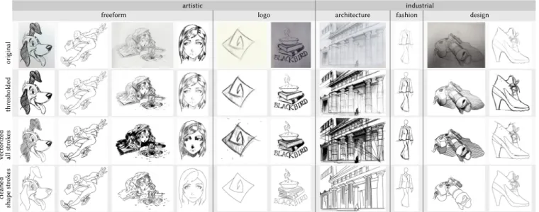
artistic industrial

freeform logo architecture fashion design

cleane d shap e str okes ve ctorize d all str okes thr esholde d original

Fig. 3. A sample from our dataset for various categories. From top to bottom: rough sketches from the wild; thresholded raster sketches to remove the background; manually vectorized rough sketches; professionally cleaned sketches (one of multiple), i.e. ground truth. From left to right: dog image ©Preston Blair, running man image ©Graham Wilson CC-BY-4.0, girl image ©David Revoy CC-BY-4.0, girl image ©Anton Gulic CC-BY-4.0, logo image ©Jakub Steiner CC-BY-SA 2.0, book logo image ©Anna A CC-BY-NC 2.0, architecture image ©Alexander Strugach under CC-BY-2.0, fashion image ©Myriam Lasserre CC-BY-SA-4.0, camera image ©Akshay Sharma CC-BY-SA, shoe image ©Graham Wilson CC-BY-4.0.

satisfy technical constraints or an industrial application. Examples of each can be found in Figure 3. We consider style to be synonymous with authorship. Within each genre, we have 4–13 different authors. See Table 1 for the distribution of authors and sketches in each genre.

Tags. Sketches are tagged with the following information: • Genre

• Author (name, preferred attribution, contact information) • Where the drawing was obtained from

• License

• Has shading strokes • Has scaffold lines • Has texture strokes

• Background (clean or paper texture from a scanned drawing) • Curated (professionally vectorized, cleaned, and evaluated) • Ambiguity: degree to which cleanup artists agree

• Messiness: ratio of rough to clean stroke coverage

Table 1 summarizes the tag statistics for our dataset. Ambiguity and Messiness are described in detail in Section 5.

License. The vast majority of sketches in our dataset have Cre-ative Commons licenses: 94% of the full dataset and curated subset (Table 1). We allow any Creative Commons license except those with a “No Derivatives” clause, since any sketch-processing algorithm creates a derivative work. The non-Creative Commons sketches come with explicit permission from the rights holder for inclusion in our benchmark. There are 18 such sketches in the full dataset and 6 in the curated subset.

Table 1. Tag statistics for the 281 sketches in our entire dataset and 101 sketches in our curated subset. Other than the Authors column, the val-ues represent the number of sketches with the property (license, presence of layers, scanned from the physical world). Sketches without a Creative Commons license (Not) are included in our dataset with explicit permission from the copyright holder. All sketches are in raster format. Sketches with a clean background were created in digital drawing software, rather than scanned from the physical world.

Creative Commons Layers

Genre Sketches Authors BY BY-NC BY-NC-SA BY-SA Not Shading Scaffold Texture Physical

All 281 39 123 60 19 61 18 187 71 75 95 Art: Freeform 86 16 23 32 2 11 18 53 11 23 19 Art: Logo 29 6 18 4 0 7 0 28 0 2 7 Ind.: Architecture 26 6 7 0 10 9 0 12 10 13 15 Ind.: Fashion 40 4 1 22 5 12 0 17 0 16 22 Ind.: Product 100 8 74 2 2 22 0 77 50 21 32 Curated 101 35 48 15 8 24 6 76 35 24 39 Art: Freeform 33 13 11 8 2 6 6 30 6 8 7 Art: Logo 12 6 7 3 0 2 0 12 0 2 5 Ind.: Architecture 12 6 5 0 2 5 0 6 6 4 9 Ind.: Fashion 11 4 1 4 3 3 0 7 0 5 4 Ind.: Product 33 7 24 0 1 8 0 21 23 5 14 4.2 Ground Truth

We hired seven professional artists to create three ground truth

cleaned versions of each rough sketch2in our curated subset and

in the additional 40 sketches used as examples in prior work. We recruited the seven professional artists via UpWork. The artists were located throughout the world (Argentina, China, Colombia, Hungary, Russia, and Serbia). Artists had 5–9 years of professional experience. The artists worked for a total of 645 hours (including vectorization of rough input sketches). One of the artists cleaned every image in our dataset and created the manual vectorizations.

We designed our problem statement to be algorithmically achiev-able. However, we did not structure the creation of ground truth data 2_{Two sketches were cleaned by four artists.}

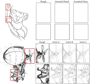
Rough Invented Detail Accepted Clean

Rough Artist A Artist B Artist C

Fig. 4. Examples of cleanup, taken from our interactions with artists. Top: The cleaning process should not add detail, as shown in the inset. Acceptable cleaning should only revise strokes already present in the put. Bottom: Ambiguities in the rough input sketch lead to multiple acceptable choices by the cleanup artists. We discuss a metric for ambiguity in Section 5.2.2. Koala image ©Enrique Rosales, aircarft image ©David Revoy CC-BY-4.0.

as a perceptual experiment. Sketch cleanup was a collaborative pro-cess between the artists and us to decide what constituted cleanup versus changing the idea of the original artist. Our goal was to obtain cleaned sketches that reflect artists’ professional skills and human perception without adding details or changing what is depicted. The cleanup task is similar to the inking step in comic book creation [Simo-Serra et al. 2018b], in which strokes are redrawn and refined. However, when inking, artists may add details that improve the drawing. We provided artists with illustrated instructions, including positive and negative examples. We encouraged them to use their best guess in case of ambiguity (Figure 4, bottom). The instructions can be seen in our supplemental materials. Misinterpretations were common (e.g. Figure 4, top). Without back-and-forth communica-tion, we would have obtained poorer quality ground truth that no algorithm could match. Structuring this as an experiment would not have served the benchmark to structure ground truth data col-lection as an experiment due to the highly skilled, time consuming, and costly demands on our artists. Our initial instructions were refined in collaboration with the artists. As ground truth creation progressed and artists gained more experience, artists worked more independently.

Artists created their cleaned vector drawings atop the input image,

which was given as a background layer in Adobe Illustrator.3We

asked artists to preserve shading and texture and clean scaffolds in their ground truth (in separate layers) for use in future research. 3_{All the artists we hired used Adobe Illustrator as their vector graphics editor. Artists}

could trace over the rough sketch.

Table 2. Automatic rough sketch cleanup methods we evaluate.

Method Input Output

TopologyDriven [Noris et al. 2013] raster vector FidelitySimplicity [Favreau et al. 2016] raster vector DelaunayTriangulation [Parakkat et al. 2018] raster vector PolyVector [Bessmeltsev and Solomon 2019] raster vector StrokeAggregator [Liu et al. 2018] vector vector MasteringSketching [Simo-Serra et al. 2018a] raster raster RealTimeInking [Simo-Serra et al. 2018b] raster raster TopologyDriven [Noris et al. 2013] →

StrokeAggregator [Liu et al. 2018] raster vector PolyVector [Bessmeltsev and Solomon 2019] →

StrokeAggregator [Liu et al. 2018] raster vector

We found that professional artists have trouble creating topo-logically accurate junctions. They were all able to create junctions which appear closed (e.g. overlapping thick strokes), but only some typically created shared stroke endpoints or endpoints ending on other curves at machine precision. Common vector graphic formats (Illustrator or SVG) cannot store topological junctions in complex scenarios, such as when more than two curves share a junction or when one curve starts or ends in the middle of another. An alterna-tive data structure could solve this problem [Dalstein et al. 2014], though it is not supported in common tools (e.g. Adobe Illustrator). During cleanup, we asked artists to label strokes in different cat-egories: shape strokes, shading, texture, and scaffolds. These are stored in separate layers. The dataset also stores each layer as a separate file to simplify future use.

Rough Sketch Vectorization. All of the 281 rough sketches are na-tively in raster format, either because they were scanned from the physical world or because they were created in a raster graphics program. Some automatic algorithms take vector input, so we hired one of the professional artists to create a faithful manual vectoriza-tion of all 101 rough sketches in the curated subset. The artist traced stroke centerlines where possible, and outlined shaded regions when individual strokes were not distinguishable. These vectorized rough sketches use a simple stroke style with constant thickness, since no standard file format can store varying attributes like thickness, it is difficult for a human to control, and thickness or color information can be estimated from the raster image under each stroke. Just as during ground truth cleanup, we asked the artist to place strokes into different layers: shape strokes, shading, scaffolds, and texture. The layers are stored as groups in an SVG file and, redundantly, split into a separate SVG file per layer. The ground truth files and manually vectorized rough input files are all provided in the same coordinate system for evaluation.

We provide each input image in its original, raster, form; as a raster image with a manually thresholded background to eliminate physical artifacts like paper texture and illumination; and its manual vectorization in SVG format (with layers as groups and as separate files).

5 EVALUATION

We evaluated seven recent algorithms and two pipelines created by composing two of the vectorization algorithms with a cleanup algorithm (Table 2). Four methods take raster input and produce vector output by applying heuristic-based optimization: PolyVector [Noris et al. 2013], FidelitySimplicity [Favreau et al. 2016], Topolo-gyDriven [Bessmeltsev and Solomon 2019], and DelaunayTriangu-lation [Parakkat et al. 2018]. One method, StrokeAggregator [Liu et al. 2018], takes vector input and produces vector output by ap-plying perceptual principles . Two data-driven approaches based on convolutional neural networks, MasteringSketching [Simo-Serra et al. 2018a] and its follow-up RealTimeInking [Simo-Serra et al. 2018b], take raster input and are the only two methods which pro-duce raster output. We use the authors’ own implementations of their algorithms. We also evaluated two pipelines: one of two self-described vectorization algorithms, TopologyDriven [Noris et al. 2013] or PolyVector [Bessmeltsev and Solomon 2019], followed by StrokeAggregator [Liu et al. 2018], the cleanup method that requires vector input.

We provide a web interface for browsing algorithmic outputs and interacting with some of our metrics. See our supplemental materials.

Parameters. We evaluate algorithms using the authors’ recom-mended or default parameters. The only approach with a user-facing parameter is FidelitySimplicity [Favreau et al. 2016], which provides users with a parameter (λ ∈ [0, 1]) to select the desired tradeoff between fidelity (adherence to the rough input) and simplicity of output curves. We evaluated it with multiple parameter settings

(λ = 0.25, 0.3, 0.5, 0.6, 0.75), which are the evenly spaced values

(0.25, 0.5, 0.75) along with the values used by the authors for ex-amples shown in their paper (0.3, 0.6). We evaluated PolyVector [Bessmeltsev and Solomon 2019] with and without the “noisy” flag. The parameters for DelaunayTriangulation [Parakkat et al. 2018] are resolution dependent. We devised a simple formula to stay within the authors’ recommended range. We set the “ len” parameter to 4% of the image diagonal, “skeleton pruning” to 3% of the image diagonal, “smoothing” to 6% of the image diagonal or 100 (whichever is larger), and “masking regions” to 40.

Input sketches. We evaluated the algorithms on our curated dataset as well as the 40 rough sketches gathered from prior work. We evalu-ated three kinds of input derived from each rough sketch: the original image, manually thresholded, and professionally vectorized (Figure 3). The raster-based algorithms often expect clean backgrounds, so we manually thresholded the original images to eliminate physical scan-ning artifacts (paper texture and lighting). We also evaluated two variants of the professional vectorization of each input image: all layers and only shape strokes. All layers corresponds to a version of the original image with a clean background and uniform stroke width. By omitting non-shape strokes, we avoid stroke types that most cleanup algorithms weren’t designed to handle.

The scale or resolution of the input is an overlooked parameter for some algorithms, as algorithms may have internal thresholds with resolution-dependent units or evaluate pixels within a sliding window of fixed, absolute size (e.g. MasteringSketching [Simo-Serra

et al. 2018a]). To account for this, we evaluated raster images at their original resolution, thresholded images at the same resolution and resized to have 1000 and 500 pixels along their long edge, and vectorized images rasterized at 1000- and 500-pixel dimensions. We evaluate StrokeAggregator [Liu et al. 2018] only on the profession-ally vectorized inputs (all layers and shape strokes only).

5.1 Sketch-to-Sketch Similarity

Much of our evaluation relies on measuring sketch-to-sketch simi-larity. There are infinitely many different vector graphics representa-tions for the same sketch. Consider, for example, that a Bézier curve can be losslessly split into multiple, shorter curves. Two sketches may look identical, but have different connectivity at T-junctions, since SVGs and other common vector formats cannot represent valence-3-or-higher junctions [Dalstein et al. 2014]. We investigated algorithms to snap endpoints and T-junctions into a representa-tion with richer topology. However, snapping endpoints affects the body of the curve, potentially destroying T-junctions elsewhere. In other places, curves run parallel to each other; after snapping, these parts of the curve become double-covered. The issues that arise and complexity of solutions begins to resemble sketch cleanup itself. Therefore, we make the decision to evaluate the quality of vector graphics representation (long, continuous versus short strokes, junc-tions quality) independently from our evaluation of sketch-to-sketch similarity (Section 5.2.1).

We do not need to consider registration or overall alignment. Ground truth was created atop the rough sketch. The algorithms we evaluate also similarly maintain the alignment of the output.

Since we have multiple ground truths for each sketch, we need to compute the similarity of one sketch to a set of other sketches. An algorithmic output could be similar to different ground truth examples for different parts of the sketch. While we could measure the distance from a point on the algorithmic output to any of the ground truth examples, a similar adaption in the other direction would require a correspondence between ground truths to deter-mine whether every point on the ground truth was close to a point on the algorithmically cleaned sketch. Unfortunately, finding cor-respondences is an open research problem. We did not want our evaluation to be subject to surprising correspondence problems. Simpler metrics are more robust and easier to reason about. As a result, we decided to use uncorresponded point-to-point similarity to compare two images and use the maximum pairwise similarity across all ground truth.

To compute point-to-point similarity, we compute a uniform sam-pling of sketches in screen-space by rasterizing them. We normalize each sketch to have uniform stroke thickness set to 0.1% of the image’s long edge, rasterize it, and then threshold such that any values darker than 75% are considered filled. This approximately matches the thickness of the raster output of MasteringSketching and RealTimeInking [Simo-Serra et al. 2018a,b] which we cannot change and similarly threshold.

We want a symmetric similarity function. It is not enough to measure how close e.g. each point on the algorithmic output is to any point on the ground truth. A partial sketch should not have equal similarity. (Table 3, “bottom.”)

perfect nudged bottom dot dot only Chamfer 0.00 0.01 0.06 0.002 0.60 F-score 0% 1.00 0.23 0.68 0.99 0.00 F-score 5% 1.00 1.00 0.73 0.99 0.00 Hausdorff 0.00 0.03 0.40 0.45 1.05 IOU 1.00 0.11 0.51 0.99 0.00

Table 3. The distance between a green and purple shape according to various distance metrics, with overlap shown in black. The first column shows a perfect match. Chamfer and Hausdorff are distances that count up from 0. F-score and IOU values lie in the range 0 (completely dissimilar) to 1 (perfect match). Nudging the perfect match shows that the IOU metric and F-score are sensitive to slight misalignments, which is undesirable in our scenario. The F-score can be tuned with a threshold parameter, though adjusting it can be difficult (nudged vs. bottom). Adding a distant dot shows that the Hausdorff distance is determined by outliers, which is also undesirable in our scenario. The Chamfer distance handles all these scenarios appropriately, and is the most distant when expected (dot only).

We experimented with several point-to-point similarity and dis-tance formula for comparing two binary images A and B: Intersec-tion over Union (IOU), Hausdorff distance, F-score, and the Chamfer distance, See Table 3 to see the behavior of these formula on simple examples. The Intersection over Union (IOU), also called the Jaccard index, measures the intersection between two regions (in our case, the number of overlapping rasterized pixels), as a fraction of their

union (the union of rasterized pixels):|A∩B |_{|A∪B |}. Values range between

1 (perfect match) and 0. Unfortunately, the IOU is extremely sensi-tive to local misalignments, as seen in Table 3, “nudged.” The other distances can all be expressed efficiently by first computing the

dis-tance transform DT of each image, where DTAis an image storing

the distance to the closest pixel in A with distances normalized to be fractions of the long edge. The Hausdorff distance computes the “worst possible” closest distance between two sets:

Hausdorff(A, B)= max(maxi ,j ∈A(DTB[i, j]), maxi ,j ∈B(DTA[i, j]))

A perfect match has distance 0. Two maximally dissimilar images

have a distance of√2 corresponding to the image diagonal. The

Hausdorff distance is dominated by the behavior of outliers, as seen in Table 3, “dot.” This makes it a poor choice for us. The F-score is the harmonic mean of precision and recall. Precision measures the fraction of points of image A (e.g. an algorithm’s output) that are within distance d of any points of image B (e.g. a ground truth sketch). Precision(A, B)= 1 |A| Õ i ,j ∈A DTB[i, j] < d

Recall measures the opposite direction. Values range between 1 (perfect match) and 0. The threshold d must be carefully chosen, as seen in Table 3, “nudged” and “bottom.” The Chamfer distance measures the average closest distance between any point in A to

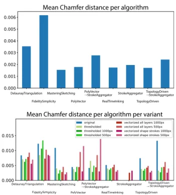
Mean Chamfer distance per algorithm

DelaunayTriangulation FidelitySimplicity

MasteringSketching PolyVector

PolyVector

→StrokeAggregator TopologyDriven→StrokeAggregator

TopologyDriven StrokeAggregator RealTimeInking

Mean Chamfer distance per algorithm per variant

→ →

Fig. 5. Comparing algorithmic sketch cleanup to ground truth. Lower is better. Above: For each rough sketch input to each algorithm, we average the best (lowest) Chamfer distance among all variants of the image compared to all ground truth cleanings of that image. Below: Broken down by image variant and resolution.

any point in B, and vice versa.

Chamfer(A, B)= 1 2|A| Õ i ,j ∈A DTB[i, j]+ 1 2|B| Õ i ,j ∈B DTA[i, j]

The Chamfer distance has a similar range as the Hausdorff, (0 to √

2). The Chamfer distance is not sensitive to outliers and local misalignments and has no parameters to tweak (Table 3).

For each rough sketch, we measured the similarity among its ground truth cleanings with all metrics (Section 5.2.2). The Chamfer distance had the best Pearson correlation score with the other dis-tances. Due to its good theoretical properties and for lack of a better alternative, we focus on the Chamfer distance for our evaluation. Other distances can be browsed in our supplemental materials.

In all of our evaluations, we compare to only the shape strokes layer of the ground truth output. No algorithms intentionally process or preserve shading, scaffolding, or texture strokes. Future research may make use of them.

5.2 How well do algorithmically cleaned rough sketches match ground truth?

A central question we wish to answer is whether a given automatic cleanup algorithm produces results similar to ground truth.

We computed distances for each image separately and use its best score across all input variants (resolution and original, thresholded, vectorized all layers, vectorized shape strokes only). This represents

Original Ground Truth

Mastering

Sketching Stroke Aggregator Real-Time Inking Poly Vector

Poly Vector →

Stroke Aggregator Topology Driven

Topology Driven → Stroke Aggregator

Delaunay

Triangulation Fidelity Simplicity

 0.00051 distance:  0.00052 distance:  0.00055 distance:  0.00066 distance:  0.00072 distance:  0.00078 distance:  0.00095 distance:  0.00228 distance:  0.00391 distance:

Original Ground Truth

Mastering

Sketching Real-Time Inking Fidelity Simplicity Topology Driven Poly Vector

Poly Vector → Stroke Aggregator

Delaunay Triangulation

Topology Driven →

Stroke Aggregator Stroke Aggregator

distance:  0.00184 distance:  0.00197 distance:  0.00204 distance:  0.00216 distance:  0.00232 distance:  0.00244 distance:  0.00318 distance:  0.00337 distance:  0.00418

Original Ground Truth

Mastering

Sketching Real-Time Inking Poly Vector Topology Driven Stroke Aggregator

Poly Vector → Stroke Aggregator

Topology Driven →

Stroke Aggregator Fidelity Simplicity Delaunay Triangulation

distance:  0.00083 distance:  0.0009 distance:  0.00094 distance:  0.001 distance:  0.00124 distance:  0.00203 distance:  0.00256 distance:  0.00351 distance:  0.00415

Fig. 6. Algorithmic cleanup output for three rough sketches, ranked according to Chamfer distance from ground truth, from better to worse (left to right). Please see the supplemental material to interact with this data. From top to bottom: animal image ©Gregory Laufersweiler CC-BY-SA-3.0, cloth image ©Rachel Bake CC-BY-NC-2.0, car image ©Jaguar MENA CC-BY-2.0.

Input 1000 px

Chamfer distance: 0.0019 Chamfer distance: 0.0015500 px

MasteringSketching

RealtimeInking

1000 px

Chamfer distance: 0.0019 Chamfer distance: 0.0020500 px

Original Size (1385 px)

Chamfer distance: 0.0020

Fig. 7. MasteringSketching and RealtimeInking (Simo-Serra et al. [2018a] and [2018b], respectively) are techniques based on convolutional neural networks (CNNs). The two algorithms consolidate repeated, rough strokes with a different resolution dependence. MasteringSketching fails on the image at its largest size. Penguin image ©Enrique Rosales.

a user willing to tweak parameters to obtain as high-quality an output as possible.

Figure 5 shows the Chamfer distance for each algorithm on our dataset. Figure 6 shows algorithmic output ranked by Chamfer

manually close

d

original

Rough Input Fidelity vs Simplicity (λ = 0.5)

Chamfer distance: 0.032

Chamfer distance: 0.008

Fig. 8. Fidelity vs. Simplicity [Favreau et al. 2016] is sensitive to gaps in the input strokes. Above: The input sketch contains gaps, so the output is missing large regions. Below: We manually close the gaps, and the output drastically improves. Pig image ©Enrique Rosales.

distance for three input sketches. We observe that all algorithms performed better with 1000-pixel resolution images than 500-pixel resolution images. This may be due to unconscious tuning by algo-rithm designers. We also observe that manual thresholding nearly always improved performance over the original images. We saw no clear performance trend for algorithms based on the input sketch’s genre.

We observed several characteristics of each cleanup algorithm. The CNN-based approaches [Simo-Serra et al. 2018a,b] consolidate

Rough Sketch Input len: 10

Chamfer distance: 0.0027 Chamfer distance: 0.002 len: 2.5

Fig. 9. The DelaunayTriangulation [Parakkat et al. 2018] method is sensitive to the input parameters. It is difficult to find one set of parameters for all sketches. Fashion image ©Hugo Fonseca CC-BY-NC-SA-3.0.

Rough Input PolyVector TopologyDriven Ground Truth

Messiness: 5.5

Messiness: 1.01

Fig. 10. The TopologyDriven [Noris et al. 2013] and PolyVector [Bessmeltsev and Solomon 2019] approaches attempt a faithful vectorization and are better suited to sketches with low messiness. Input images from Favreau et al. [2016].

repeated strokes with a resolution dependency (Figure 7). The reso-lution at which they do this is different. FidelitySimplicity [Favreau et al. 2016] performs poorly in the presence of gaps (Figure 8). Delau-nayTriangulation [Parakkat et al. 2018] is sensitive to its input pa-rameters (Figure 9). We chose papa-rameters dynamically as a function of the image long edge, but much better parameters can be found via fine tuning. The vectorization approaches (TopologyDriven [Noris et al. 2013] and PolyVector [Bessmeltsev and Solomon 2019]) in-deed focus on faithful vectorization and do not group repeated messy strokes (Figure 10). For that reason, they are better suited for sketches with low messiness (Section 5.2.2).

5.2.1 Vector Path Quality. We measure two characteristics of the

vector representation itself. The two CNN-based methods we evalu-ate [Simo-Serra et al. 2018a,b] cannot participevalu-ate in this evaluation, because they output raster images. The sketches created by human artists (ground truth and manual vectorizations) can participate.

We measured the arc length of continuous paths represented in each algorithmic cleanup’s SVG output. It is preferable to store a visually continuous curve as a single, long path rather than multi-ple shorter ones placed end-to-end but topologically disconnected. A downstream algorithm will likely expect that separately stored paths in the SVG typically correspond to visually separate paths. Statistics about path arc lengths for the algorithms we evaluate can be seen in Figure 12. StrokeAggregator [Liu et al. 2018] had far superior curves than the other algorithms, on par with rough human sketches. The ground truth artists produced paths whose arc lengths were typically many times longer than any algorithmic output.

We also measured the quality of junctions between curve end-points. SVG’s and other common vector graphics formats cannot represent 3-way (or higher) junctions, so any T-junctions must nec-essarily cause a discontinuity in how the paths are stored where there is none visually. However, if the distance between the end-point of a curve and all other curves is zero, then the junction is stored in the best way possible. For this reason, and to correct for short paths as described above, downstream applications often as-sume that coincidence implies connectivity. We sum the minimum distance between every curve endpoint and every other curve in the SVG, normalized such that the image’s long edge has length 1. Figure 11 plots statistics about the total minimum distance and the number of endpoints whose minimum distance to another curve was over 0.1% of the image’s long edge. We use the total minimum distance rather than the average minimum distance, because that would benefit algorithms that store long, visually continuous paths as topologically disconnected short paths. StrokeAggregator [Liu et al. 2018] also had the best performance in this metric, though many algorithms created higher quality junctions than humans as expected (Section 4.2).

Timing and Failure Rate. We measure the time each algorithm took to complete (Figure 13). We also measure the fraction of rough sketches an algorithm was able to successfully process. An algo-rithm which took longer than 30 minutes or more than 40GB or RAM was terminated and considered as a failure. Running all al-gorithms for all inputs took 25 days of CPU time. This does not count time taken when algorithms failed to complete. Due to the intense computational requirements and differing operating sys-tem requirements, we ran the algorithms on several machines with different specifications. Machine A had an Intel Core i7-6700 3.4 GHz CPU with 4 cores and 48 GB of RAM. Machine B had an Intel Core i7-7700HQ 2.80 GHz CPU with 4 cores and 16 GB of RAM. All algorithms except those mentioned below ran on Machines A and B. In particular, any algorithms which failed due to high memory use ran on Machine A. Machine C had an Intel Core i5-5287U 2.90GHz CPU with 2 cores and 16 GB of RAM. Machine C was used solely for DelaunayTriangulation [Parakkat et al. 2018]. MasteringSketching and RealTimeInking [Simo-Serra et al. 2018a,b] ran on remote GPU clusters for which we do not have precise machine specifications. We did not run algorithms in parallel, so that parallel algorithms could have uncontested access to all CPU cores.

The CNN-based approaches [Simo-Serra et al. 2018a,b] were by far the fastest to run, finishing in just a few seconds. Other methods

1 2 3 4 5 6 7 8 To ta l m in im um ju nc tio n di st an ce p er in pu t Junction distances 0 DelaunayTriangulation FidelitySimplicity PolyVector2StrokeAggregator PolyVector TopologyDriven2StrokeAggregator

StrokeAggregator TopologyDriven Rough GT

0 1000 2000 3000 4000 5000 6000 # op en en dp oi nt s per in pu t

Open endpoint distribution

DelaunayTriangulation FidelitySimplicity

PolyVector2StrokeAggregator

PolyVector TopologyDriven2StrokeAggregator

StrokeAggregator TopologyDrivenRough GT

Fig. 11. Top: The minimum distance from a path’s endpoint to any other path provides a simple way to measure gaps at junctions between paths. Lower is better. We sum the minimum distance for all endpoints in a sketch to estimate the openness of its curves. Algorithm performance is far better than that of humans. Bottom: We count the number of open endpoints per output. Lower is better. An open endpoint is defined as having a closest path farther away than 0.1% of the image’s long edge.

0 0.1 0.2 0.3 0.4 0.5 0.6 0.7 Mea n ar c len gt h per in pu t

Arc length distribution 3.1_…

DelaunayTriangulation FidelitySimplicity

PolyVector2StrokeAggregator

PolyVector TopologyDriven2StrokeAggregator

StrokeAggregator TopologyDriven Rough GT

Fig. 12. The average length of a topologically continuous path. Higher is better. A visually continuous path should be stored as a long, continuous path rather than as multiple shorter paths placed end-to-end but topologically disconnected. We compare algorithm and human performance. Human ground truth falls off the plot, as a handful of sketches have average arc lengths distributed up to 3.1. Seconds 1000 400 300 200 100 0 500 600 700 900 800 Running Time DelaunayTriangulation FidelitySimplicity MasteringSketching PolyVector PolyVector

→StrokeAggregator TopologyDriven→StrokeAggregator TopologyDriven StrokeAggregator RealTimeInking

Fig. 13. Average running time in seconds for each genre of input. Logos tend to be simpler and hence run faster. The pipelines were built atop the output of PolyVector and TopologyDriven; the dashed regions correspond to this first stage.

took between a minute or two (DelaunayTriangulation [Parakkat et al. 2018]) and over ten minutes (StrokeAggregator [Liu et al. 2018]). Logos are the simplest sketches in our dataset and took the least time to run.

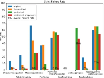
We measured the strict and overall failure rate of each algorithm (Figure 14). An algorithm failed if it did not produce output for a rough sketch across all (overall) or any (strict) tested algorithm pa-rameters and image variants, within our time and memory bounds. RealTimeInking [Simo-Serra et al. 2018b] was the only method which never failed. The other CNN-based method (MasteringSketch-ing [Simo-Serra et al. 2018a]) failed for images whose resolution

was over 8002. StrokeAggregator [Liu et al. 2018] had the highest

failure rate, though it has the fewest chances to succeed since there are only two vector variants for each rough sketch. It was the only algorithm to have any overall failures. All other algorithms were able to produce some output for some image variant or resolution. When run as a pipeline atop the algorithms PolyVector [Bessmeltsev and Solomon 2019] and TopologyDriven [Noris et al. 2013], their failure rates decrease.

5.2.2 Ambiguity and Messiness.

How ambiguous is a rough sketch? A given rough sketch may be more or less ambiguous. Our multiple ground truth cleanings of each sketch allow provide us with data to obtain such a measure-ment. We define the ambiguity of a rough sketch as the average pairwise distance between all ground truth cleanings. As with all of our evaluations, we compute ambiguity using only the shape strokes layer of the ground truth. Examples of ambiguity can be seen in Figure 15. See the supplemental materials for per-sketch ambiguity. Ambiguity may be caused by densely repeated strokes, gaps in a stroke, or semantic ambiguity (when context changes the interpretation of strokes). Ambiguity may also be due to different high-level decisions about the cleanup process, such as whether a stroke is scaffold, shading, or texture versus a shape stroke, and whether to apply some amount of global beautification.

10 20 30

40 39%

50

Strict Failure Rate

Percent 60 70 80 90 100 0 0% 0% 0% 0% 0.7% 0% 0% 11%

X% overall failure rate

DelaunayTriangulation FidelitySimplicity

MasteringSketching PolyVector

PolyVector

→StrokeAggregator TopologyDriven→StrokeAggregator TopologyDriven StrokeAggregator RealTimeInking

Fig. 14. Failure rates for the algorithms. An algorithm was considered to have failed if it did not produce output within 30 minutes and 40 GB of RAM across all (strict failure rate) or any (overall failure rate) parameter settings, image variants, and resolutions. The overall failure rate for all algorithms except StrokeAggregator and its pipelines was 0%.

Messiness. A messier sketch has more strokes or markings that are removed during cleanup than a less messy sketch. Figure 15 depicts several examples. We define a rough sketch’s messiness as the ratio of covered area removed during cleanup. Messiness compares all layers of the input image, since that is how it is given, to the shape strokes of the ground truth, since that is the desired output. Practically, we compute this as the ratio of the number of pixels in all layers of the vectorized rough sketch S to the average

number of pixels in the shape strokes of each ground truth Gi. Using

the vectorized input avoids physical artifacts.

Messiness(S, {Gi})= #pixels(S)

average({#pixels(Gi)})

fashion

architecturelogofreeformproduct

0 .0 0 .5 1 .0 1 .5 2 .0 2 .5 3 .0 3 .5 4 .0

The average messiness per genre can be seen inset right. Messiness for individ-ual sketches varies from approximately one to ten depending on an artist’s style. Messiness also varies by category. Prod-uct sketches tend to have more scaf-fold lines and shadows while the fashion sketches we collected are closer to their cleaned versions. See the supplemental materials for per sketch messiness. High ambiguity typically corresponds to high messiness, but the opposite is not always true (Figure 15-g).

5.2.3 Perceptual Study. We performed a pilot perceptual study with

naive subjects on Amazon Mechanical Turk. We summarized our problem statement (Section 3) and asked subjects to “mark the de-gree to which each of the following drawings is a high-quality neatened version of the above rough drawing” with a 5-point Likert scale. We performed the experiment with two rough sketches, one

freeform and one architectural, for which all cleanup algorithms, in-cluding the pipelines, succeeded. For each rough sketch we obtained

ratings from N= 20 subjects for all nine algorithmic outputs and the

three professional artists’ ground truth outputs. The (twelve) neat-ened drawings were arranged in randomized order in a 3 × 4 gallery. The perceptual study itself (what subjects saw, the ratings for each output, and analysis) can be seen in the supplemental materials.

Our pilot study obtained inconsistent results. The Chamfer dis-tance was highly correlated with mean Likert scores for the

architec-ture input (Pearson’s r= −0.87, p = 0.0002)—more so than all other

metrics except F-score with a particular threshold. The Chamfer

dis-tance was not as highly correlated for the freeform image (r= −0.33,

p= 0.30), and was less correlated than other metrics. We discuss a

confounding factor below. Tukey’s Honestly Significant Difference (HSD) test determined that, for each of the two inputs, some neat-ened drawings received significantly different mean Likert scores from others. However, a Wilcoxon signed-rank test determined that the ranking of each neatener (algorithm or artist) was significantly

different (inconsistent) between the two inputs (p = 0.18).

Rank-ings were based on mean Likert scores. Anecdotally, subjects rated the output of MasteringSketching [Simo-Serra et al. 2018a] highly for both inputs (ranked best or second-best). It was rated above all-but-one ground truth and the follow-up work by the same au-thors [Simo-Serra et al. 2018b]. There may be a confounding factor: MasteringSketching [Simo-Serra et al. 2018a] output thicker lines than the other approaches, including its follow-up work. Since those two approaches output raster images, we cannot simply normalize the line thickness as we can for SVG output. Excluding the Likert scores of MasteringSketching [Simo-Serra et al. 2018a], the Cham-fer distance’s correlation with human ratings increases. It becomes the most highly correlated metric for both the architectural input

(r= −0.90, p = 0.0001) and freeform input (r = −0.56, p = 0.07).

The above analysis is based on a small sample (two example sketches and twenty ratings per output). It may be that scaling our study up to large numbers of subjects and inputs would produce consistent, significant results. However, to conduct a successful per-ceptual study, it may be that subjects with expertise or additional training or more focused questions are required. For example, Xu et al. [2019] asked subjects to rate the aesthetics, conformity, and tidiness separately. A two-alternative forced choice (2AFC) experi-ment may be able to determine whether outputs are significantly different with fewer queries.

6 CONCLUSION

Rough sketch cleanup has the potential to bridge the gap between sketches made in practice and a large literature of sketch processing algorithms. To succeed, cleanup algorithm must be able to process sketches as they are in the wild. We introduced a dataset which reflects the variety and reality of sketches in the wild. The accompa-nying professionally vectorized and cleaned derivatives we acquired identify weaknesses and open problems with existing cleanup al-gorithms, and provide future research a scaffold for progress. Our ground truth similarity metric serves as a benchmark challenge. Au-tomatic algorithms should aim to produce results as close to ground truth as the multiple ground truth images are to each other. We

Medium Ambiguity (0.003) Medium Messiness (3.77) a) High Ambiguity (0.004) High Messiness (5.18) b) High Ambiguity (0.005) High Messiness (9.36) e) Low Ambiguity (0.0002) Low Messiness (1.21) c) High Ambiguity (0.009) High Messiness (5.11) d) High Ambiguity (0.006) Low Messiness (1.57) ) Low Ambiguity (0.001) High Messiness (4.67) g) Low Ambiguity (0.0003) Low Messiness (1.36) h)

Fig. 15. Ambiguity versus Messiness. Ambiguity may be due to thick regions of repeated strokes (a, b), gaps (c), or semantic ambiguity (d). Ambiguity may also be due to different decisions regarding the cleanup process, such as which strokes are scaffold/shading/texture versus shape strokes (b), whether occluded contours should be kept (e), or whether to apply global beautification (f). All but global beautification correspond to higher messiness. Some messy drawings have low ambiguity (g). In the absence of global beautification, drawings with low messiness typically have low ambiguity (h). Author/copyright information for the sketches: a and f) from Liu et al. [2015], b) Patrick Murphy, CC-BY-2.0. c) Maria Fiddler, CC-BY-NC-SA-4.0. d) Trip Ivey, CC-BY-4.0. e) Akshay Sharma, CC-BY-SA. g) Alexander Strugach, CC-BY-2.0. h) Preston Blair, explicit permission.

Rough Iterated Our Ground Truth

Fig. 16. A comparison of the original artist’s iteration on their (thresholded) rough sketch and one of the ground truth cleaned versions created by an independent professional for our dataset (shape strokes only). Top row rough and iterated images © Anastasia Majzhegisheva CC-BY-4.0. Bottom row rough and iterated images © Jinho Jung CC-BY-SA-2.0.

plan to publish our evaluation scripts, providing future researchers a simple way to automatically evaluate their algorithms on our benchmark.

Limitations and Future Work. We defined our problem statement for rough sketch cleanup (Section 3) narrowly with the hope that multiple ground truth cleanings by professional artists would agree (low ambiguity) and that a similar result could be achieved algo-rithmically in the future. An alternative problem statement could define the next “iteration” of the artwork, such as inking [Simo-Serra et al. 2018b]. Our dataset does not consider this more ambiguous

problem statement. For two of our rough sketches, we have the orig-inal artist’s own refinement. Figure 16 compares our professionally cleaned sketches to the original artist’s own refinement.

In the future, we would like to explore end-to-end evaluations on specific downstream sketch processing tasks like 3D reconstruction [Xu et al. 2014] or animation in-betweening [Whited et al. 2010; Yang et al. 2018]. We would also like to resolve imperfections in human-created ground truth related to junctions and stroke thick-ness and color. Imperfect junctions could possibly be resolved with a semi-automated snapping routine and a non-standard data structure capable of representing n-way junctions and curves which termi-nate in the middle of others [Dalstein et al. 2014]. Stroke thickness and color could be estimated from the underlying raster image; again, semi-automation and a non-standard data structure would be needed.

ACKNOWLEDGMENTS

We are grateful to all the artists who generously contributed their rough sketches to our dataset. We acknowledge the artists whose hard work created the ground truth data: Branislav Mirkovic, Santi-ago Rial, Diego Barrionuevo, Ge Jin, Jonathan Velasco, Liliya Larsen, and Maria Fiddler. The authors who shared their implementations with us deserve special mention for furthering science: Bessmeltsev and Solomon [2019]; Favreau et al. [2016]; Liu et al. [2018]; Noris et al. [2013]; Parakkat et al. [2018]; Simo-Serra et al. [2018a,b]. Many fruitful discussions with colleagues improved this work. We thank Adrien Bousseau for helpful discussions on dataset creation and Eli Schechtman for suggesting the Chamfer metric. We are grateful to Jixuan Zhi, Rawan Alghofaili, and the GMU ARGO cluster for lending us computing resources. Finally, we thank the anonymous reviewers for taking the time to read our paper and provide feed-back. Their comments and suggestions ultimately led to a better paper for everyone.

Authors Yan and Gingold were supported by the United States National Science Foundation (IIS-1453018), a Google research award,