Complete safety software testing : a formal method

COMPLETE SAFETY SOFTWARE TESTING:

A FORMAL METHOD

by

JON R. LUNGLHOFER

B.S., United States Naval Academy, Annapolis, Md. (May 1994)

SUBMITTED TO THE DEPARTMENT OF

NUCLEAR ENGINEERING IN PARTIAL FULFILLMENT

OF THE REQUIREMENTS FOR THE DEGREE OF MASTER OF SCIENCE

at the

MASSACHUSETTS INSTITUTE OF TECHNOLOGY

February, 1996

@ Massachusetts Institute of Technology, 1996. All rights reserved

Signature of Author_ .

_/

Departnp-it of Nu#ear Engineering

January, 1996

Pes r Michael W. Golay

Thesis Sunervior .

PTfessor Dh*id D. Lanning Thesis Reader

/..fes6r Jeffrey P. F*idberg

COMPLETE SAFETY SOFTWARE TESTING:

A FORMAL METHOD by

JON R. LUNGLHOFER

Submitted to the Department of Nuclear Engineering on January 18, 1996 in partial fulfillment of the requirements for the Degree of Master of Science in

Nuclear Engineering.

Abstract

In order to allow the introduction of safety-related digital control in nuclear power

reactors, the software used by the systems must be demonstrated to be highly reliable. One method of improving software reliability is testing. A study of the complete testing of software was performed based upon past research. The literature search found two complete testing methods, only one of which, complete path testing, was feasible for use. The literature contained a practical and nearly complete testing method known as Structured Path Testing, developed by Howden

(Howd77). Structured Path Testing was adapted here as the basis for a new testing method known as Feasible Structured Path Testing (FSPT). The FSPT involves a five step formal method which examines the code's data flow structure and develops test cases based upon the analysis. The FSPT eliminates unfeasible paths from the test case which greatly speeds the testing process.

The FSPT was applied to several simple programs. Many of the test programs are written in the 001 case tool language developed by Hamilton Technology (Hami92.). The ultimate example test bed program, known as the Reactor Protection System (RPS) was written by M. Ouyang (Ouya95).

The work reported here was restricted to the examination of software code testing. No attempt was made to examine the reliability of corresponding hardware or human interactions. In order to improve reliability of safety-critical software, one must assure that human interactions are simple and that hardware is sufficiently redundant.

The results of the study presented here indicate that for simple programs, complete testing is possible. If looping structures are included in a program, in most cases, the tester must sacrifice complete testing in order to complete the testing process within the programs lifetime. While the scope of this study was limited, there is no reason to believe the FSPT could not be used for much larger tasks. The FSPT greatly enhances the reliability of software code.

Thesis Supervisor: Michael W. Golay

Acknowledgments

I wish to thank my thesis supervisor, Professor Michael W. Golay for his continued direction and support throughout this study. Without his financial, technical, and personal assistance, this work could not have gone forward.

I wish to thank ABB-Cumbustion Engineering for their financial support which allowed this work to go on. Special thanks go to Michael Novak, the primary contact at ABB-CE. His feedback and clear focus helped to focus the goals of this research.

Hamilton Technology Inc. also deserves thanks for supplying the 001 system for use in the project. Special thanks goes to Margaret Hamilton for her generous offer of the 001 evaluation system package; to Ron Hackler, Nils, and Zander for their continued technical assistance, both on-line and off.

Thanks also go to Meng Ouyang for his patience, helpfulness, and companionship throughout my stay at MIT. I enjoyed working with Meng and wish him the best of luck in his future endeavors. Thanks also go to Chang Woo Kang for being a true friend, (Kamsa Hamnida). Thanks to Rachel Morton for her continued support in drafting this thesis.

Finally, I wish to thank my family at home and away from home. Thanks Mom for all your love, I couldn't have made it without you. Thanks go to David Fink for begin an excellent room mate while at MIT. We shared some excellent time together. To all my friends at the Boston Rock Gym, whom are too numerous to list, I thank you all for your companionship. To Tina Burke, my true inspiration, I thank her for her constant love and support. Climb On.

Table of Content

A BSTRA CT ... 3

A CK NOW LEDG M ENTS ... 5

TABLE OF CO NTENT ... 7

LIST OF FIG URES ... 9

LIST OF TABLES ... 11

1. INTRO DUCTIO N...13

1.1 GENERAL ... ... ... ... 13

1. 2 BACKGROUND ... 14

1.3 M ETHOD OF INVESTIGATION... 16

1.4 SCOPE OF THE W ORK ... 17

2. LITERA TURE SEARCH ... 19

2.1 GENERAL ... 19

2.2 SOFTwARE DEVELOPMENT M ETHODS... 20

2.2.] Structural Requirements... 21

2.2.2 Formal Development M ethods... 36

2.3 SOFTWARE CODE TESTING M ETHODS... 37

2.3.1 Black Box methods... 37

2.3.2 ite Box M ethods... 39

2.3.3 An Overview of Testing Technique... 55

2.4 LrTERATURE SEARCH CONCLUSION ... 56

3. SELECTIO N O F A TESTING M ETH O D ... 59

3.1 GENERAL ... 59

3.2 FEASIBLE STRUCTURED PATH TESTING ... 59

3.2.1 Method Overview... 60

3.2.2 Feasible Structured Path Testing: The Details... 61

3.2.3 Feasible Structured Path Testing: General Testing Strategy... 66

3.3 FSPT: AN EXAM PLE... 68

3.4 FSPT: A SECOND EX AM PLE ... 71

3.5 FSPT: CONCLUSION ... 73

4. TH E 0 0 1 CASE TO O L ... ₇₅

4.1 GENERAL ... 75

4.2 TYPE M APS (TM APS) ... 75

4.3 FUNCTION M APS (FM APS)... 78

4.4 00 1 SYSTEM REVIEW ... 82

5.1 INTRODUCTION ... ... 83

5.2 T'IiE REACTOR PRoTEcnoN SysTEm ... 83

5. 2 1 RPS 001 TM ap and FM aps ... 84

5.3 TBE FSPT OF TBE RPS ... 92

5.3.1 Testing the Operations ... 93

5.3.2 Testing the H igh Level Code, Update -State ... 106

5.3.3 Conclusion of the FSPT of the RPS ... 108

5.4 FSPT ERROR LOCAT[ON EXPERM ENT ... 109

5.5 CONCLUSION ... 113

6. CONCLUSION ... 115

6.1 RECOMm EgDAn om To DESIGNERS ... 115

6.2 FUTURE W ORK ... 6 ... 116

6.3 IZENM W .6 ... 117

List of Figures

FIGURE 2-1 PROCESS BLOCK DIAGRAM ... 25

FIGURE 2-2 DECISION BLOCK DIAGRAM ... 26

FIGURE 2-3 JUNCTION DIAGRAM ... 27

FIGURE 2-4 SIMPLIFIED EXAMPLE PROGRAMMING LANGUAGE ... 28

FIGURE 2-5 AUTOMATIC TELLER MACHINE (ATM) EXAMPLE CODE ... 29

FIGURE 2-6 ATM EXAMPLE CODE AND FLOWGRAPH ... 30

FIGURE 2-7 MCCABE METRIC EXAMPLE FLOWGRAPHS ... 32

FIGURE 2-8 EXAMPLE LOOPING PROGRAM FLOWGRAPH... 44

FIGURE 2-9 LOOPING EXAMPLE PROGRAM FOR ILLUSTRATING DATA FLOW TESTING...48

FIGURE 2-10 A FLOWGRAPH OF THE LOOPING EXAMPLE WITH DATA FLOW ANNOTATION... 48

FIGURE 2-11 SUBMARINE DOOR EXAMPLE PROGRAM SPECIFICATION DOCUMENT ... 51

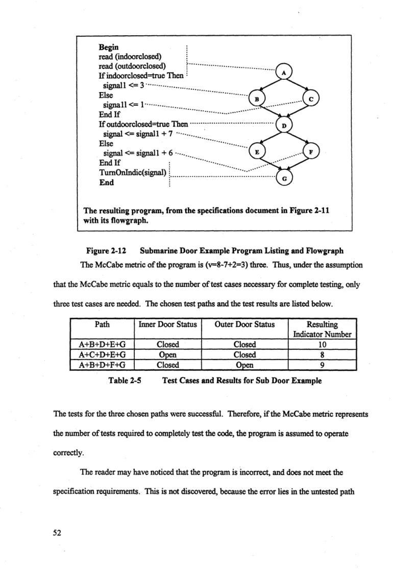
FIGURE 2-12 SUBMARINE DOOR EXAMPLE PROGRAM LISTING AND FLOWGRAPH ... 52

FIGURE 2-13 EXAMPLE FLOWGRAPH TO DEMONSTRATE ALTERED PATH TESTING METHODS .... 54

FIGURE 3-1 H ORRIBLE LOOPS...61

FIGURE 3-2 FOWGRAPH EXPANDED TO K ITERATIONS... 63

FIGURE 3-3 FLOWGRAPH EXPANSION: TRANSITIONAL VARIABLES...65

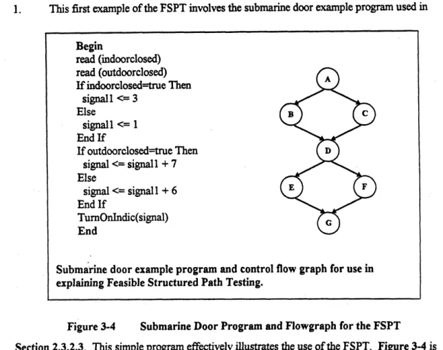
FIGURE 3-4 SUBMARINE DOOR PROGRAM AND FLOWGRAPH FOR THE FSPT...68

FIGURE 3-5 STEP THREE EXPANDED FLOWGRAPH: SUBMARINE DOOR EXAMPLE ... 69

FIGURE 3-6 THIRD STEP EXPANDED FLOWGRAPH: LOOPING EXAMPLE... 72

FIGURE 4-1 TYPE MAP (TMAP) EXPLANATION... 76

FIGURE 4-2 EXAM PLE TM AP ... 77

FIGURE 4-3 FUNCTION MAP (FMAP) EXPLANATION... 79

FIGURE 4-4 001 REUSABLE CONTROL STRUCTURES... 80

FIGURE 4-5 EXAM PLE FM AP ... 81

FIGURE -1 R PS TYPE M AP ... 85

FIGURE 5-2 HIGH LEVEL FMAP UPDATESTATE... 86

FIGURE 5-3 OPERATION CHECKGLOK ... 86

FIGURE 5-4 OPERATION UPDATEINDI FMAP ... 87

FIGURE 5-5 STRUCTURE SETINDIUPDATE FMAP... 88

FIGURE 5-6 OPERATION UPDATEGL FMAP... 89

FIGURE 5-7 STRUCTURE SETTRIPCHECK FMAP... 90

FIGURE 5-8 OPERATION UPDATEUPONTRIP FMAP... 91

FIGURE 5-9 ORDER OF TESTING THE RPS ... 93

FIGURE 5-10 UPDATEUPONTRIP FLOWGRAPH... 95

FIGURE 5-11 UPDATEUPONTRIP STEP 3 FLOWGRAPH ... 97

FIGURE 5-12 UPDATEGL FLOWGRAPH ... 100

FIGURE 5-13 UPDATEGL STEP 3 FLOWGRAPH ... 101

FIGURE 5-14 UPDATEINDI FLOWGRAPH ... 104

FIGURE 5-15 UPDATE_INDI STEP 3 FLOWGRAPH... 105

FIGURE 5-16 UPDATESTATE FLOWGRAPH... 107

FIGURE 5-17 SAMPLE INPUT TMAP TO OPERATION UPDATESTATE ... 108

FIGURE 5-18 SAMPLE OUTPUT TMAP FROM UPDATESTATE... 109

FIGURE 5-19 UPDATEGL WITH ERRORS... 111

FIGURE 5-20 UPDATEGL WITH AN ERROR STEP 3 FLOWGRAPH ... 112

List of Tables

TABLE 2-1 THE LINEARLY INDEPENDENT PATHS OF THE ATM CODE... 34

TABLE 2-2 PATH COVERAGE OF THE ATM CODE... 42

TABLE 2-3 BRANCH COVERAGE OF THE ATM CODE ... 42

TABLE 2-4 FEASABLE TEST PATHS OF ATM CODE ... 43

TABLE 2-5 TEST CASES AND RESULTS FOR SUB DOOR EXAMPLE ... 52

TABLE 3-1 LINERALY INDEPENDENT PATHS OF THE SUBMARINE DOOR EXAMPLE ... 69

TABLE 3-2 TESTED CASES: SUBMARINE DOOR EXAMPLE ... 70

TABLE 3-3 LOOPING PROGRAM FOR EXAMPLE THE FSPT...71

TABLE 3-4 LINEARLY INDEPENDENT PATHS OF THE LOOPING EXAMPLE... 73

TABLE 5-1 TEST PATHS: UPDATEUPON_TRIP ... 98

TABLE 5-2 TEST CASES: UPDATEUPONTRIP ... 98

TABLE 5-3 UPDATEUPONTRIP TEST RESULTS... 99

TABLE 5-4 TEST PATHS: UPDATEGL ... 102

TABLE 5-5 TEST CASES: UPDATEGL ... 102

TABLE 5-6 TEST RESULTS: UPDATEGL ... 103

TABLE 5-7 TEST PATHS: UPDATEUPONTRIP ... 105

TABLE 5-8 TEST CASES: UPDATEUPONTRIP ... 106

TABLE 5-9 TEST RESULTS: UPDATEUPON TRIP ... 106

TABLE 5-10 TEST PATHS: UPDATESTATE ... 107

TABLE 5-11 TEST CASES: UPDATESTATE ... 107

1. Introduction

1.1 General

Due to the difficulties of verification and validation (V& V), the nuclear power industry has lagged in the introduction of digital control software to regulate the safety systems of nuclear power plants. The (V& V) process includes testing the software against design specification performance requirements. Software designed for use in nuclear power plant safety systems should be completely tested to prove its correctness. Without a method of verifying a software system, the nuclear industry continues development without the advantages of modern digital control

technologies common to other industries.

Extensive methods have been developed to determine the reliability of the analog safety systems currently being utilized in nuclear power plants. The debate over the introduction of digital control software systems stems from the question of reliability. In order for digital control software to replace the current analog systems, the software must be proven to be as reliable. Given the complexity of the (V& V) process, this is a difficult task.

The development of highly reliable software systems has been of great interest to those operating large, complicated, and expensive systems that are traditionally prone to human error. Such systems include fly-by-wire aircraft and telecommunication systems. Due to the large size of these programs, it is considered impossible to completely test them. These programs are tested until the expected frequency of error detection is longer than the program's expected lifetime. This

method of testing does not offer an all together acceptable standard of reliability. The U.S. Nuclear Regulatory Commission (NRC) holds the nuclear industry to a higher standard.

This work seeks to develop, or find, an existing method for completely testing safety-critical software. Also, the work will, in the absence of a complete testing method, demonstrate the best method available. The method of choice will be tested on simple pieces of safety software. The art of software development will also be examined. The complexity of a piece of software corresponds with its testability. It is possible to design software that it is easily testable, or nearly impossible to test. This report examines methods for developing software that improve the ease of testability. This work leads to an improvement in nuclear power plant safety by paving the way for the use of modem digital technology.

1.2 Background

There are many ways in which softvare can contain errors, and many ways to test for those errors. The ultimate goal is to locate every error in a piece of safety-related software to allow for its use in a nuclear power plant. If safety-related software can be demonstrated as highly reliable with very little uncertainty, it would likely become an integral part of the nuclear power plants of the future. However, due to the nature of software systems, partial proofs with high uncertainty will be insufficient. Software errors, unlike hardware faults, are always present and waiting to be unearthed. Where hardware can be inspected to reveal faults, software must be tested against the specification document to demonstrate errors. Since undetected software errors often lie in rarely used sections of code, such as accident sequence responses, it is imperative that all the errors be detected in the (V& V) phase of software development.

In order to test a piece of software for errors, one must first understand the types of errors that can occur. Software faults can result from the following sources of error:

* Incorrect formulation of the program specifications.

" Operating system errors. " Environmental errors.

* Input / output errors.

" Programming errors, such as: " syntax errors

* logical errors

" numerical errors (division by zero, etc.)

There are many documented ways of searching for errors. The methods can be broken down into two main categories, black box and white box testing. Black Box testing treats the program as if it were a closed box. There is no examination of the code during the testing process. Test cases are generated purely from the specification document. The results of these test cases are

compared with a database of correct results to determine if the correct output was obtained. This database is commonly referred to as an oracle. The existence of an oracle is necessary for all types of testing. The test cases generated during white box testing result from an examination of the code structure. White box testing also requires an oracle to assure that the test results are correct.

Many other methods exist for improving software reliability. Some of these methods are not based on testing and include:

" Developing two different programs on two or more different operating environments from the same specifications. The two software systems are then compared to each other. Every differences between the two codes is a potential sources of error and must be addressed.

" The code is checked independently line by line for syntax and conceptual errors.

* Graphic oriented formal development languages are used to develop the code which is internally consistent and complete in capture of the specifications.

* Programs are modularized to decrease the complexity of the code. Small pieces of code are less prone to errors.

There are many sources of error in the software development process. Even using the most careful of development methods, errors pass into the final software code. It is necessary to test for these errors. Only when a complete test of the software against its specification document is completed can one be assured of correct performance.

1.3 Method of Investigation

The effort reflected in this work is the result of a literature search of all documents pertaining to software testing. The search covers a broad range of software testing methods and styles. The aim of the search is to identify, test, and possibly improve upon the most efficient and complete testing method currently documented in the literature. Methods for developing reliable software are also examined. The literature is discussed and summarized.

An examination of several simple safety-related programs is utilized to illustrate the effectiveness of chosen testing methods. Other examples are used to demonstrate the performance of other testing methods described in the literature.

1.4 Scope of the Work

There are many sources of software errors external to the software development process. This work focuses upon the testing of the software code for programming errors. The testing of the hardware, operating system, and environment are considered beyond the scope of this work and will not be included. While these types of errors are quite common in complicated software

systems, it is assumed that the environment in which the software operates is in working order. The benefits of designing simple and easily testable modular software is examined here. Poorman's work (Poor94) demonstrates the usefulness of the software complexity metric. The complexity metric offers a formal method of gauging the complexity of a piece of software. Using a metric, one can assure that sections of software code do not become overly cumbersome and difficult to test.

Although it is generally considered impossible to completely test a piece of complex software, this work demonstrates that if software is written simply and correctly it can be thoroughly tested. If the software specifications document is written incorrectly or incompletely, one can not assure correct software performance. The testing method described in this report requires the presence of an oracle. The development of an oracle is a topic deserving of a study

2. Literature Search

2.1 General

This section summarizes the literature search of software testing methods used as the starting block for this study. The literature search for the work reported here was broad in scope, yielding many possible methods for testing software code. The goal of the search was to identify all of the available testing methods, and assess the possibilities based upon completeness,

practicality, and overall usefulness. The research lead to many articles discussing reliable software development methods. Even though they do not directly relate to testing, these articles were given attention. A more reliable development process can only lead to less errors in the code which simplifies the testing process. Experience shows that in many cases software can not be completely tested, because of the over whelming number of test cases necessary. There are also hardware and user interaction concerns. Finally, there is the concern that the specifications document may include errors which can be passed on to the software. Since this study focuses only upon the complete testing of software code, other concerns, such as hardware and human interaction, have been eliminated from the search.

Thus, the search focuses on methods for testing software code and the development of coding practices which ease the testing process. The results of the search include two complete testing methods. One of these, exhaustive input testing, is applicable only in very simple theoretical cases making it incompatible with this study's requirements. The other method,

In programs which involve loops, the Strucutred Path Testing technique sacrifices completness for

timeliness, but is an excellent compromise which greatly improves program reliability.

The search begins with a review of previous research work done at MIT, the initial focus

being the work of Poorman (Poor94) and Arno (Arno94). Both use a cyclomatic metric based

testing schemes to yield complete testing results. The cyclomatic metric, also known as the

McCabe metric for its developer T. J. McCabe, is explained in detail later in this chapter. The use

of the cyclomatic metric is very helpful in gauging the difficulty of testing a piece of code. While

helpful in determining the minimum number of tests needed for certain types of code testing, the

McCabe metric based testing technique used by Poorman and Arno does not reliably provide a

complete code test. The McCabe metric testing method does not test every possible execution path

through the code. Using the standard control flowgraph, the McCabe metric testing technique used

by Poorman and Arno guarantees branch coverage. It is possible that untested paths contain

errors. The concepts of branch and path coverage as well as the control flowgraph are covered

later in Section 2. The McCabe metric based technique is explained and its limitations fully

demonstrated later in this chapter. Recall that the focus of our search is to locate a complete

testing method. The results of Poorman and Arno do not yield a complete testing method. Thus,

our search expands to examine all types of code testing methods in hopes of locating a complete

method.

2.2 Sofbvare Development Methods

In recent years, the use of formal methods to develop software has become widespread.

size. For small and simple programs the ad hoc approach will never be replaced. However, for safety critical software systems, it is necessary to have a highly reliable form of quality control.

The software development process begins with the establishment of a requirements or specification document and continues through the design, testing, and documentation stages (Poor94). While the main focus of the work reported here is upon the testing phase, the design phase is also examined in Section 2.2.2. The software design process has been studied here in hopes of identifying ways for decreasing the introduction of errors into the final testable piece of software, thus easing the testing process. A broad range of topics can be classified as software development methods and they are examined here.

In a report prepared for the Nuclear Regulatory Committee (NRC) concerning the preparation of a severe reactor accident computer code, Sandia National Laboratories described a method for the reliable management of a large software development project (Qual91). Described within the report, is the management plan for treating situations which may be encountered during

software development. Such procedures are essential with large projects dealing with many individuals. The main goal of the management plan is to deal with changes in the software as it is being developed. The document says little about the specific development of the software system, and focuses upon human interactions within a large programming team. While it is necessary to have methods for the administration of large software projects, such managerial details are beyond the scope of this study. The goal here is to develop methods which are specific to the coding process itself.

It has been demonstrated that the number of errors in a piece of code is related to the complexity of the section of code in question. A study was conducted by Lipow that demonstrated the existence of a non-linear relationship between the size of the program and the number of errors

or bugs, found within the code (Lipo82). He demonstrated that smaller programs had a much lower error rate than had larger programs. He found that as the number of lines of code increased to around 100 the number of errors per line grew at a linear rate. However, in larger programs (>

100 lines), the number of errors per line increased in a non linear fashion. He concluded that

shorter programs have an advantage over larger ones in terms of the amount of errors found per line. The practice of writing modular code takes advantage of these findings. However, in the literature there are many different ideas addressing when a program should be broken into modules. The differences stem from a general disagreement over how to measure the complexity of a piece of code. The question is: "How ... [does one] ... modularize a software system so the resulting modules are both testable and maintainable?" (McCa76)

The complexity of a piece of code is often measured by a software metric. A software metric is a number generated by a method or technique that supplies information about the complexity of the code in question. For his study, Lipow used the lines of code metric, which is equal to the number of lines of written code. The lines of code metric is utilized by several companies to govern the maximum allowable module size (Beiz90). This metric is the simplest, but can often underestimate the true complexity of the code in question. Consider a twenty five line program that consists of twenty five consecutive if . . then statements. This program contains 225 possible paths of execution. Merely measuring the number of lines of code is not enough to judge the complexity. Many other metrics have been developed to aid the programmer in deciding when to modularize.

These metrics are numerous and can be categorized as either linguistic metrics or structural metrics (Beiz90). A linguistic metric is based upon measuring various aspects of the program's text. For example, the basis of a linguistic metric could be the number of lines of written source code. The linguistic metric is based upon any aspect or combination of aspects of the physical text layout. The structural metric is based upon the structural relationship between program objects. The structural metric is usually based upon understanding the programs control flow graph. For example, a structural treatment may gauge the extent of recursive structures in the code by examining the flow paths shown in the control flow graph. Two of the most useful metrics Halstead's (a linguistic metric) and McCabe's (a structural metric) are discussed here. The explanation of McCabe's metric is prefaced by a review of the control flowgraph.

2.2.1.1 Halstead's Metric

Halstead's metric is the best established of all linguistic metrics (Beiz9O). Halstead developed the metric first by examining the patterns of errors in a large and diverse set of programs (Hals77). Halstead then took two simple linguistic measurements from each program, the number of program operators (e.g. keywords such as Repeat..Until and if..then), and the number of program operands (e.g. variables and data types).

nI = the number of distinct operators in the program.

n2= the number of distinct operands in the program.

These two measurements were then used in a formula derived from an empirical fit to the actual error data. The hope was that the number of errors in a program could be predicted with relative accuracy using the metric. The metric gives a value designated as H

which Halstead called the "program length." The "program length" H should not be confused with the number of lines of code in the program.

Halstead also defines two move parameters based on the total number of operator and operand appearances in the program text.

N1= Total operator count

N2= Total operand count Halstead also defines a new metric

N = N1 + N2 (2.2)

known as the actual Halstead length (Beiz90). Halstead's claim is that the value of H will be very close to the value of N. This has been confirmed by several studies. Thus, if the programs makeup is known it is possible to calculate an estimated length of the finished program, before it is written.

Halstead also developed a calculation to predict the number of errors present in a program (Beiz90). The formula

Errors

(NI

(2.3)

is based on the four values: ni, n2, N1, and N2.

For example, if a program has 75 data object and uses them 1300 times and 150 operators which are used 1200 times, then according to Equation 2.3 there should be

(1300+1200)log2(75+150)/3000 = 6.5 errors in the code.

Halstead's metric is very useful for the management of a large programming project, but is not such a useful tool with regard to completely testing that software. The metric does not supply the user with knowledge of the true number of errors, only an estimate. There is of course no way to have 6.5 errors in a piece or software. Thus the Halstead metric is a useful tool, but is unable to

help adequately with the complete testing process. One could use Halstead's error estimation metric as a gauge of when to stop testing the code (Poor94) (e.g. stop testing after the estimated number of errors are found). However, such a technique seems far from complete. Halstead's

metric is a useful tool for measuring and comparing the complexity of software codes being considered for the same job. The simplest code should be used. Although Halstead's metrics are useful, they do not facilitate the complete testing of a piece of software code, and is not used in this study.

2.2.1.2 The Control Flowgraph

Understanding the control flowgraph is central to understanding much of the literature on software testing. In general, the control flowgraph is a graphical representation of the control

structure of a program. Before the control flowgraph can be discussed it is first necessary to introduce some standard terminology. The following terms are used to describe various aspects of computer code:

Process Block

A section of code in which the statements are executed in order

from the entrance to the exit is known as a Process Block. Figure 2-1 Process Block Diagram

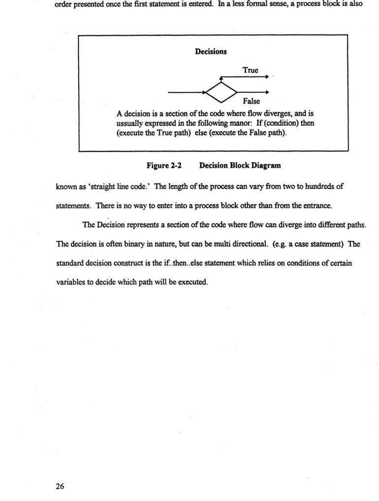
order presented once the first statement is entered. In a less formal sense, a process block is also

Figure 2-2 Decision Block Diagram

known as 'straight line code.' The length of the process can vary from two to hundreds of statements. There is no way to enter into a process block other than from the entrance.

The Decision represents a section of the code where flow can diverge into different paths. The decision is often binary in nature, but can be multi directional. (e.g. a case statement) The

standard decision construct is the if..then..else statement which relies on conditions of certain variables to decide which path will be executed.

26

Decisions

True

False

A decision is a section of the code where flow diverges, and is

ussually expressed in the following manor: If (condition) then (execute the True path) else (execute the False path).

Junctions

When program paths merge together, a Junction is formed.

Figure 2-3 Junction Diagram

The Junction is a piece of code where flow paths can merge together. For example, when the separate true and false paths end after an if..then statement, the flow can merge together again.

These merges are known as Junctions.

All programs can be broken down into some combination of these three elements. In some

cases statements can be both decisions and junctions, such as loop control statements. The terminology used above is taken from the flowchart concept. The flowchart has become outdated and is being replaced with the control flowgraph. The control flowgraph greatly simplifies the flowchart concept. There are only two types of components to the flowgraph: circles and lines. A circle is called a node and line a link. A node with more than one link entering is a junction and one with more than one leaving a decision. The node with only one link entering and one link exiting is a process node. All code structures can be expressed using the control flowgraph.

An example is used to illustrate the control flowgraph. For this example a written program must be examined. To facilitate this, a generic and simple "programming language" is adopted. The language used is based on that developed by Rapps and Weyuker in 1985

(Rapps85). Using this language should break down any language barriers other high level languages might cause. The following statement types are included in the language:

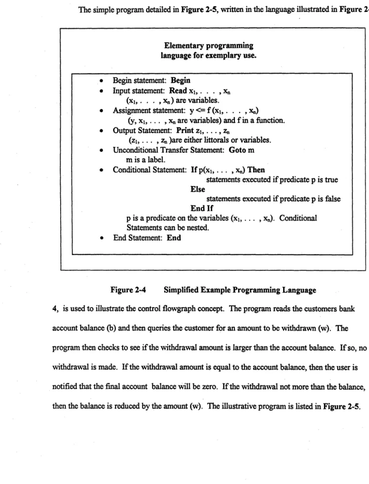
The simple program detailed in Figure 2-5, written in the language illustrated in Figure

2-* Begin statement: Begin

* Input statement: Read xi,. . . , (xI,. . , x.) are variables.

* Assignment statement: y <= f (x1,. . . , x.)

(y, xj, . .. , xn are variables) and f in a function. * Output Statement: Print zi, . . ., z.

(zi, . . . , zn )are either littorals or variables. * Unconditional Transfer Statement: Goto m

m is a label.

* Conditional Statement: If p(xi,... , x.) Then

statements executed if predicate p is true Else

statements executed if predicate p is false End If

p is a predicate on the variables (xi, ... , x.). Conditional

Statements can be nested. * End Statement: End

Figure 2-4 Simplified Example Programming Language

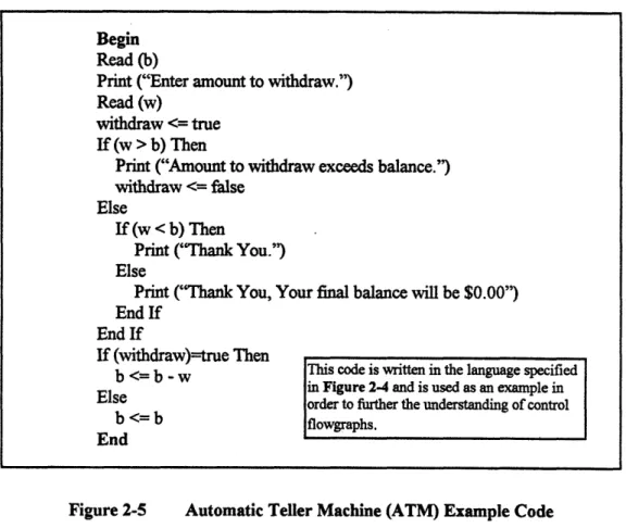
4, is used to illustrate the control flowgraph concept. The program reads the customers bank account balance (b) and then queries the customer for an amount to be withdrawn (w). The program then checks to see if the withdrawal amount is larger than the account balance. If so, no withdrawal is made. If the withdrawal amount is equal to the account balance, then the user is notified that the final account balance will be zero. If the withdrawal not more than the balance, then the balance is reduced by the amount (w). The illustrative program is listed in Figure 2-5.

28

Elementary programming language for exemplary use.

Begin Read (b)

Print ("Enter amount to withdraw.") Read (w)

withdraw <= true

If (w > b) Then

Print ("Amount to withdraw exceeds balance.")

withdraw <= false

Else

If (w < b) Then

Print ("Thank You.") Else

Print ("Thank You, Your final balance will be $0.00") End If

End If

If (withdraw)=true Then

b

b

in Figure 2-4 and is used as an example in

Else _{order to further the understanding of control}

b <= b flowgraphs.

End

Figure 2-5 Automatic Teller Machine (ATM) Example Code

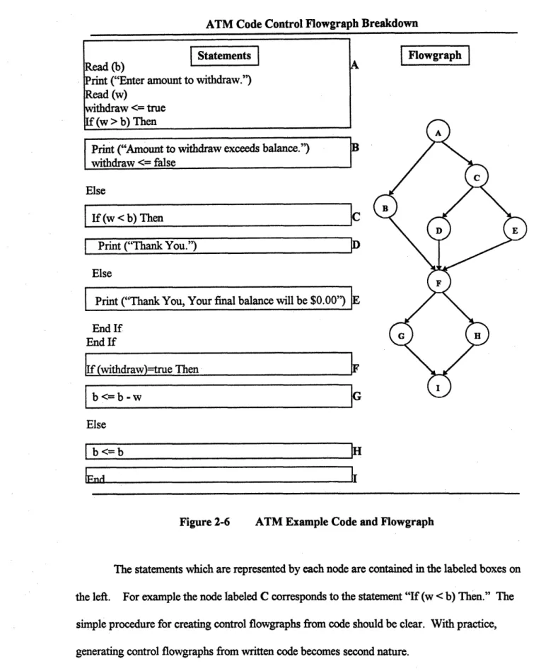
The simple program above can be broken down into its control flowgraph. Figure 2-6 illustrates the control flowgraph.

ATM Code Control Flowgraph Breakdown

Print ("Amount to withdraw exceeds balance.")

withdraw <= false

Else

If (w < b) Then

A

1C

I

Print ("Thank You, Your final balance will be $0.00") E End If End If If (withdraw)=true Then b <= b -w F G Else

I

Figure 2-6 ATM Example Code and Flowgraph

The statements which are represented by each node are contained in the labeled boxes on the left. For example the node labeled C corresponds to the statement "If (w < b) Then." The simple procedure for creating control flowgraphs from code should be clear. With practice, generating control flowgraphs from written code becomes second nature.

Read (b) [tents]

Print ("Enter amount to withdraw.") Read (w) withdraw <= true If (w > b) Then Flowgraph A C B D E F G H I

Many terms used in software engineering relate to the control flowgraph (Rapps85). The links on the control flowgraph are also known as edges. An edge is a connection between nodes. An edge from node] to node k is given the notation (f, k). Node] designated as the predecessor of node k, and node k the successor to]. There can be only one edge between any two distinct nodes. The first node of a program is known as the start node, and has no predecessors while the last node is known as the exit node and has no successors.

A path orflowpath is a finite sequence of nodes connected by edges. A path is designated by a sequence of nodes. For instance, a possible path through the ATM Code is Path 1 =

(A+B+F+G+I). Path 1 is a complete path because the first node is the start node and the last node the exit node. Path 1 is also a loop-free path because none of its nodes are repeated. If any node

in a path is repeated, the path contains a looping structure. It is possible that such a path could contain an infinite amount of nodes. Such a path never reaches an exit node and is the result of a

syntactically endless loop. There is no possible escape from such loops, and they often result from

program errors.

The control flowgraph, or flowgraph as it is termed hereafter, is the foundation of structural metric analysis. This section should be reviewed if questions remain on the use and construction of flowgraphs.

2.2.1.3 McCabe's Mefric

The McCabe's metric is a structure-based metric developed by Thomas J. McCabe (McCa76). McCabe noted that many software engineering companies had trouble deciding how to modularize there software systems. Many used the length-of-code metric, which seemed illogical

to McCabe. Some programs are much more complex that others of the same length. McCabe hoped that his metric would give a more accurate measure of program complexity.

The calculation of McCabe's metric is a simple process. The McCabe metric is derived from the flowgraph of the software in question. McCabe defines his metric v as

v= e-n+2p (2.4)

where

e is the number of edges or links, n is the number of nodes,

p is the number of connected flowgraph components.

Edges and nodes have been explained previously, but the value p may be unclear. Consider the following example (Figure 2-7 consisting of a main program (M) and two subroutines (A and B). The flowgraph has three detached sections and thus the value of p is equal to three.

An Illustration of the McCabe Metric

M: A: B:

A

B

Figure 2-7 McCabe Metric Example Flowgraphs

Let us calculate the value of the McCabe's metric for each individual section in the illustration. The main program M contains three edges and four nodes in only one section. The metric for M takes the value

The McCabe metric values for sections A and B separately are

v(A)=6-5+2(1)=3 ,and (2.6)

v(B)= 3 -3 +2(l)= 2 . (2.7)

If A and B are considered sub operations of the main program M, then the value of the McCabe metric of M including A and B is

v(MuAuB) = 12 -12+2(3)= 6 . (2.9)

Notice that in this case v(MuAuB) is equal to the sum of v(M), v(A), and v(B). In general, the value of the complexity metric of a number of connected flowgraphs is the same as the sum of their

individual complexity metric values (McCa76).

McCabe's metric is based upon a calculation of the number of linearly independent paths through the flowgraph in question. The complexity value 'v' is equivalent to that number. We can see this in the example above. For instance, there are clearly only three paths from the start node to the exit node in subroutine A, and the value of v(A) is equal to three. Suppose that we examine the flowgraph from the ATM code in Figure 2-4. This flowgraph has a McCabe metric value of four, as shown by the calculation

v(ATM)=11-9+2=4 . (2.9)

Inspection of the corresponding flowgraph reveals six different paths leading from the start node A to the exit node I. Recall that the McCabe metric gives the number of independent paths from start to exit. In the case of the ATM code, two of the six paths are linearly dependent upon the other four. Although any four of the six paths can be selected as the independent ones, it is useful to have a standard procedure.

A procedure for selecting the independent paths is documented by Poorman (Poor94).

First a basepath must be selected. In order to facilitate the ease of selecting subsequent paths, it is convenient to select the path the with most nodes as the basepath. However, any path can serve

this purpose. In the ATM example, the path (A+C+D+E+G+I) is selected as the basepath. The next step is to locate the first node along the basepath which contains a conditional split, and to

follow the alternate path, rejoining the basepath as soon as possible. This path is said to be independent. If the first alternate path contains a conditional split before rejoining the basepath, this second path is followed rejoining the first alternate or the basepath as quickly as possible. This process is repeated until all of the branches of the first alternate path have been exercised, and have rejoined the base path. In our example, by following the alternate route from the conditional

split at A, the next independent path would (A+B+F+G+I).

After the set of alternate paths has been exhausted, the basepath is followed to the second conditional split where the process is repeated. The second conditional split is exhausted of alternate paths and the process continues until there are no longer any new paths to follow. The resulting set of paths should be equal in number to the McCabe metric. The set of paths is also linearly independent. Thus, any other path through the flowgraph can be equated to some linear combination of the independent paths. Let us continue the process of finding the independent paths in the ATM example. At node C the alternate path (A+C+E+F+G+I) is found and at node F, path (A+C+D+F+H+I) is found. Thus the complete set of independent paths is presented in Table

A The lineraly independent paths of the flowgraph illustrated in

Figure 2.6 are presented in Table 2-1. The flowgraph is

C printed to the left for the readers convinience.

D E

F

Table 2-1

T

Path Number Flow Path

1 A+C+D+F+G+I

2 A+B+F+G+I

3 A+C+E+F+G+I

2-1.

Note that there are two other paths through the flowgraph which are not included in the list above. These paths, path 5 (A+B+F+H+I) and path 6 (A+C+E+F+H+I) are dependent paths. They can be represented as a linear combination of the other four paths. Path 5 = Path 2+ Path 4 - Path 1:

Path 5 = (A+B+F+H+I) = (A+B+F+G+I) + (A+C+D+F+H+I) -(A+C+D+F+G+I) .

Likewise, path 6 can be represented as a linear combination of paths one through four.

Path 6= (A+C+E+F+H+I) = (A+C+E+F+G+I) -(A+C+D+F+G+I) + (A+C+D+F+H+I) .

McCabe demonstrated that the value of 'v' closely correlates to the number of errors present in a piece of code. As the value of the complexity metric v increases, the number of errors in the code increases as well. McCabe also noted that, in general, longer programs have low complexity and smaller ones have high complexity levels. This, he felt made program length modularization techniques highly inadequate. Instead, McCabe suggested that every module that had a metric value higher than ten should be further modularized. This he concluded would limit programming errors, and would result in code which is more easily tested.

The basics of the McCabe metric should now be understood by the reader. For a more in depth study of the topic see McCabe's paper "A Complexity Measure" (McCa76). The McCabe metric gives a method of measuring the structural complexity of a piece of code in a standard way. This allows one to set criteria for code modularization. The McCabe metric also gives the user a method for locating the independent paths through a flowgraph. Work has been done which utilizes the McCabe metric as the basis of a structural testing strategy. This testing method is discussed in Section 2.3.2. Used as either a testing aid or a gauge for program modularization, the McCabe metric is a useful tool for a software engineer.

2.2.2 Formal Development Methods

The use of formal development methods has recently become very prevalent in software development. Formal development methods are replacing the ad hoc methods previously used in software development. With the use of formal development methods, strong feedback is

incorporated between the different elements of the design process. The use of formal methods improves the development process in two ways, according to Ouyang (Ouya95):

A complete and unambiguous specification is developed in a form which facilitates

mathematical validation.

* Verification of the software during the production process is much more effective. The formal development method provides a mathematically based specification which describes the concept of the program. This mathematical basis provides an excellent foundation for verification and validation of the code. The use of a formal method has been shown greatly to improve the software development process. The formal method requires an increase in time spent on the early stages of a project, as the specifications are the main focus of the formal method. This extra time is later recovered over in the lifetime of the software. When using informal methods, much of the time spent developing software is devoted during the final stages of validation and verification. Because of this, much of the software must be reengineered. The use of a formal method greatly reduces the number of errors which are passed to the final testable code.

Ouyang's work includes a deep description of the many formal development methods currently in use. By comparing the various development methods, Ouyang concluded that the

DBTF (Development Before The Fact) formal method was the most effective among those available currently. DBTF is marketed by Hamilton Technology Inc. of Cambridge, Ma. (Hami92a) The application of the DBTF method is aided by a CASE Tool Suite known as the

001 System. The 001 System is explained in this report. For a closer examination of the subject

of the formal development methods, one should review Ouyang's work.

2.3 Software Code Testing Methods

The main emphasis of the literature search of this report is upon code testing methods. The goal is to find the most efficient, and complete method possible. In order to choose this method, the literature is extensively reviewed, and each method is rated for completeness and general usefulness. In the end, the most complete methods are incorporated into a formal testing method. This formal method is then tested on several software codes.

A search of the literature of code testing reveals many different testing strategies. Some of

these methods are specific to certain program types or programming languages and are ignored due to their lack of generality. The goal of the study reported here is to find a method which is useful

in general, and not in specific cases only. Many of the methods found, fit this criteria. Although the methods are quite diverse, they can be broken down into two categories: black box testing and

white box testing. Black box methods are based purely upon the specification document of the

program in question. The code is treated as a closed box and is never examined. In white box testing, the code is examined, and tests are formulated based on the some aspect of the code itself.

Black box testing methods are examined first.

2.3.1 Black Box methods

Black box testing methods, also calledfunctional testing methods, derive test cases from the specifications and not the code itself. The tester is not concerned with the mechanism which

generates an output, only that the output is correct for the given input set (Myers79.) Simple programs are often tested with black box methods. For example, a simple program's specification document might indicate that two numbers (A and B) be taken from user input and their sum (A+B) be displayed on the screen. To test this simple piece of code functionally, an input set is chosen which represents the typical use of the code. The tester may wish to input several

combinations of A and B. For instance the cases where A is equal to B, A is greater than B ,and A is less than B could constitute a test set. The tester may wish to use input data values which are more likely to cause errors. For instance letters of the alphabet could be entered instead of numbers. If all of these cases execute properly, the code is found to be satisfactorily tested functionally. However, if one of the functional test cases yields an incorrect result, the code must be examined for the error. Due to the nature of the strategy, black box testing is also known as

input / output testing.

Recall that the focus of this search is to locate a complete, yet practical testing method. The only complete black box method is known as exhaustive input testing. For the example above, every possible combination of the two numbers would be tested, resulting in an infinitely large test set. Exhaustive input testing is very impractical. If any one of the input variables is a rational number, an infinite amount of test cases must be considered. Despite the apparent impracticality of complete black box testing, these methods should be mentioned. They are examined here as a possible compliment to another more useful testing method. It may be possible to use them in conjuncture with other testing methods to achieve a more complete result.

Myers identifies a method for decreasing the number of tests needed in the input / output testing process. This method is called equivalence partitioning, and deals directly with the specification document to decrease the number of test cases needed. Because of the unfeasibility of exhaustive input testing, one is limited to a small subset of the allowable input values. With the

equivalence partitioning method, this small subset is put to the greatest use possible. There are two considerations when developing test cases. The first is that the test case reduces the total number of tests needed by more than one. The second is that the test covers a large range of other test cases; i.e. it should test for more than one error type simultaneously (Myers79). Test cases are developed from each condition given by the specification document. Myers gives several rules for choosing test cases from the specifications. The process is a very subjective one with only a few loose

guidlines. The testing of erroneous input values is stressed. Equivalence partitioning testing is a heuristic testing method, and is far from complete. For a more complete reference, one should review Myers.

Black box testing methods can be very useful, as they simulate the actual usage of the program. The program's targeted user will not examine the internal workings of the code during each usage. Black box methods will always be useful in testing small pieces of code designed for a simple and specific tasks. Exhaustive input testing is the only known complete black box testing method, and is very impractical. Functional testing methods may not offer a viable complete testing alternative, but could be used in conjunction with other methods of testing to achieve a useful result, and thus they are mentioned here.

Black box testing methods represent just one of the many testing schemes in the literature.

All of the alternatives must be considered before a decision can be made as to which one is the

most effective. While, it is possible that black box methods can be used in parallel with other methods to achieve an effective yet incomplete result, the heuristic approach which is so

fundamental to black box methods makes them a poor candidate for use in the work reported here.

White box testing methods generate test sets by examining the inner workings of the program in question. White box testing is also known as structural testing due to the basis of the method upon the code structure. Many types of structural testing methods exist. This survey

reviews these numerous methods in order to decide which one is the most satisfactory for the job of complete testing. Since we can not be certain of finding a complete testing method, many

incomplete testing methods are examined here. These incomplete methods may be used in conjuncture with other methods or as the basis of a new method to improve software reliability.

2.3.2.1 Basic Structural Testing Methods

To understand the concept of structural testing, three testing methods must become familiar. These techniques are statement, branch, and path testing methods, and they form the base of understanding most other forms of structural testing methods. These testing techniques are said to result in a certain coverage of the code.

* Statement coverage (known as C1) is a testing method which assures that every statement of the code has been tested. In other words, the test set selected results in the execution of every

statement in the code. (Ntaf88)

* Branch coverage (known as C₂) is achieved by testing every transfer of control from one

program statement to the next. To attain complete branch coverage, every direction at every decision node must be executed at least once by a test case (Howd8 1). Statement coverage is included in C2.

* Path coverage (known as C.) is attained by executing every possible control path through the

Statement coverage is the least rigorous structural testing method. It is often possible to achieve statement coverage with relatively few test cases, even for a large piece of code. At the end of the test campaign, the tester knows that all of the statements in the code are executable, and that the program has yielded some correct results. However, the program tester can not concluded that the code is error free. Complete statement coverage is a far too limited a testing criterion to be used to indicate successfully complete testing.

Branch and path testing are very fundamental concepts to the study of structural testing metrics. Paths have been introduced previously in the description of control flowgraphs (Section

2.2.1.3). Recall that a complete path is a sequence of nodes starting with the entrance node and

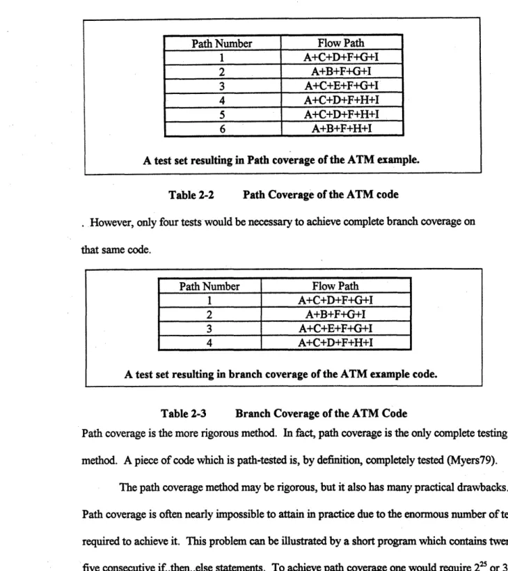
finishing with the exit node of a program. Path testing involves testing every possible path through the flowgraph. This method can result in many tests. In the case of the ATM example code, recall that there are six paths through the code. Recall Figure 2-6, the flowgraph of the ATM code. To achieve path coverage, the six paths are those summarized in Table 2-2.

A test set resulting in Path coverage of the ATM example.

Table 2-2 Path Coverage of the ATM code

However, only four tests would be necessary to achieve complete branch coverage on that same code.

Path Number Flow Path

1 A+C+D+F+G+I

2 A+B+F+G+I

3 A+C+E+F+G+I

4 A+C+D+F+H+I

A test set resulting in branch coverage of the ATM example code.

Table 2-3 Branch Coverage of the ATM Code

Path coverage is the more rigorous method. In fact, path coverage is the only complete testing method. A piece of code which is path-tested is, by definition, completely tested (Myers79).

The path coverage method may be rigorous, but it also has many practical drawbacks. Path coverage is often nearly impossible to attain in practice due to the enormous number of tests required to achieve it. This problem can be illustrated by a short program which contains twenty five consecutive if..then..else statements. To achieve path coverage one would require 225 or 33.5 million test cases. Branch coverage, however, could be achieved with as little as two tests, one for all of the true branches and one for all of the false branches. It may not be possible to formulate such perfect test cases in practice, as some paths may be infeasible.

Path Number Flow Path

I A+C+D+F+G+I 2 A+B+F+G+I 3 A+C+E+F+G+I 4 A+C+D+F+H+I 5 A+C+D+F+H+I 6 A+B+F+H+I

An infeasible test path can result from either branch or path coverage analysis. The reader may have noticed already that of the six paths in Table 2-2, only three of them are executable. Those paths are shown in Table 2-4.

Path Number Flow Path

1 A+C+D+F+G+l

2 A+B+F+H+I

3 A+C+E+F+G+I

Table 2-4 Feasable test Paths of ATM Code

For every test case, a set of input variables must be determined which will cause that flowpath to be followed. In the ATM code example, the input variables are "b" and "w". An analysis of the

code reveals that the edge of node A divides the input variables into two distinct regions,

(w > b) and (w 5 b). The edge of node C further divides the input variables into the three regions

(w > b), (w < b), and (w = b). One can also notice that if either node D or node E is reached, then

the exit sequence will be (F+G+I). If node B is reached, then the exit sequence will be (F+H+I). Thus, three of the possible paths through the code are infeasible, meaning that no input variable set can be identified which will cause their execution. The possibility of infeasible paths adds to the time consuming nature of path testing. Infeasible paths can also be a nuisance when branch testing.

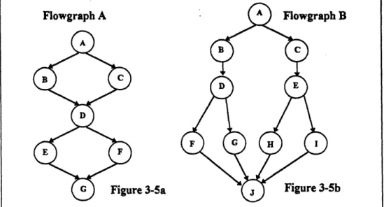
Looping path structures add great complexity to the process of software testing. Looping structures are the most difficult to test completely. Any type of recursion can result in an

exponential growth in the number of paths in a piece of code. For example, consider Figure 2-8 depicting a section of code containing a looping structure which executes "n" times through. There are three possible paths for each pass, or iteration through the loop.

For one iteration (n=1)

A

there are three paths, a B

manageable number.

D E However, the number of

test paths increases very F

quickly as the value of

G _{n increases, as 3". Ten}

Example Program to illustrate the relationship between iterations result in looping structures and structural testing techniques.

59049 paths, and 100 Figure 2-8 Example Looping Program Flowgraph iterations lead to

5.15* 1 4 paths. Path testing becomes very infeasible as the number of iterations increases. In fact, for even 20 iterations a tester would have to execute one test every second for 100 years to complete the testing process. Since software is often outdated in a matter of years, it is necessary to find a more accommodating testing process.

"Branch testing ... is usually considered to be a minimal testing requirement (Ntaf8)." This statement implies that errors can and do pass through branch coverage. Howden cited three empirical studies which showed that many errors are undetected by branch coverage (Howd8 1). A compromise must be found between the minimal approach of the branch coverage method and the infeasible, but complete path coverage method. The goal of this report is to locate a complete, and accommodating testing method. Path coverage is a complete testing method, but is not

accommodating in most cases. Let us examine the other types of structural methods in the literature in hopes of finding a compromise.

2.3.2.2 Data-Flow Methods

Data-Flow testing methods are common in the literature and represent a possible

compromise to unfeasibility of complete path testing. There are many types of data-flow methods. Only the most useful methods are summarized in this report. To understand data-flow testing methods, one must be familiar with several concepts which are explained below.

Data-flow testing works with the flowgraph to support a search for data-flow anomalies. Data-flow testing can lead to a selection of tests which represent a compromise between the rigor of path testing and the minimal approach of branch testing (Biez90). An extensive literature exists concerning the subject of data-flow testing. Much of this work was lead by Rapps and Weyuker

(Rapps85). Their premise behind the idea of data-flow testing is a simple one. Their statement, as

quoted by Biezure (Biez90), that ". ..one should not feel confident about a program without

having seen the effect of using the value produced by each and every computation," has truth to it. Data-flow testing has its origins in the black box testing technique of exhaustive input testing. In theory, every possible input value could be tested in order to satisfy the complete test

criteria, but as we have seen, this is impossible for all but the simplest of codes. Data-flow testing is an intelligent method for selecting a small subset of the input domain for testing purposes (ie. for equivalence partition testing). One hopes that the selected subset reveals all of the errors in the program. In practice, such a subset is difficult, if not impossible to locate (Rapps85). However, systematically locating as complete a test set as possible is the goal.

For every testing method other than complete path testing, one must assume that the errors located in the code, also known as bugs, can be detected by the testing method of choice. In data-flow testing, one must assume that the program bugs are a result of the incorrect use of data

objects. For instance, if the program's control structure is incorrect, data flow testing assumes that this error is refected in the data objects. This is a key assumption.

Comprehending the terminology of data-flow testing is very important to understanding the literature. Data-flow testing examines the process through which input data is transformed and processed in order to achieve the end result of the program. A data object is any type or variable

which can be used by the program to alter either other program variables or the program's control flow. Data objects can exist and function in a number of ways as defined by the following symbols (Biez9O).

" d or def- defined or initialized.

* k -killed or destroyed. " u -used in some manner.

" c -used in a calculation.

* p -used in a predicate. A variable used as a predicate controls the execution path of the program. (ie. X is a predicate in the statement "IF X-true THEN Goto A ELSE Goto B")

As data objects flow through a program, their states and uses can be traced using the symbols above. For instance, a data object could be defined, used in a calculation, and then destroyed. Such a combination of events would be denoted as dck. Some combinations of symbols represent normal data-flow situations, while others represent bugs. For instance the combination

du is allowed and frequently encountered. The data object is first defined, and then used.

However, if the combination ku ever were to occur in a program, an error would be indicated, since

impossible. With these symbols in mind, data-flow testing techniques can be thoroughly understood.

Rapps and Weyuker introduce a family of path selection criteria, based upon data flow analysis (Rapps85). In order to understand the notation used to describe a family of paths, one must first grasp the concept of a def-clear path. A def-clear path, which stands for definition clear path, is a path which does not contain a definition of a particular variable (call it x) in any of its interior statements. The following notation is given in further explanation of the concept of def-clear paths. A path (i, nj , .. . , n. ,

j)

Many types of test path selection criteria are introduced by Rapps and Weyuker, however, the most complete set of selection criteria corresponds to the all du-paths method. A du-path (n,, .

.. , _{ni, nk) is defined, with respect to a variable x, as meeting one of the following criteria.} * nk is a c-use of x and path (ni, . . . , nj, nk) is a simple and def-clear path with respect to x.

* (nj, nk) contains a p-use of x, and the path (ni, . . ., nj) is both def-clear with respect to x and loop free.

As well, the node ni must contain a definition use of the variable x. With the criteria in mind, one can define the test strategy governed by the all du-paths method. Simply put, the all du-paths method includes all paths which contain a du-path for every variable in the code. This is best illustrated by an example. The following example program is written in the language illustrated in Figure 2-4.