MAR 2 8 1969 )
COMMUNICATION UTILIZING FEEDBACK CHANNELS
by
THEODORE JOSEPH CRUISE
S.B., Massachusetts Institute of Technology
(1965)
S.M., Massachusetts Institute of Technology
(1966)
E.E., Massachusetts Institute
(1966)
of Technology
SUBMITTED IN PARTIAL FULFILLMENT OF E REQUIREMENTS FOR THE DEGREE OF
DOCTOR OF PHILOSOPHY
at the
MASSACHUSETTS INSTITUTE OF TECHNOLOGY January, 1969
Signature of Author
Department of Electrical E ineering, January 24, 1969
Certified by _ _ _ :_
Thesis Supervisor Accepted by
-.
-Chairman, Departmental Committee on Graduate Students
by
THEODORE JOSEPH CRUISE
Submitted to the Department of Electrical Engineering on January 24, 1969 in partial fulfillment of the requirements for the degree of Doctor of Philosophy.
ABSTRACT
Communication at essentially error-free rates approaching channel capacity has always involved complex signalling systems. Recently it has been noted that this complexity can be removed at
the expense of a noiseless feedback channel from the receiver back to the transmitted. Even simple linear modulation.schemes with feedback can signal at error-free information rates approaching channel capacity for a white noise forward channel. Such feedback systems and their characteristics have been analyzed for both digital and analog communications problems. The optimum linear feedback system is given for both situations.
The addition of feedback channel noise makes the communications model more realistic and has also been studied. The optimum linear system remains undetermined for noisy feedback; a class of suboptimal feedback systems yield asymptotically optimal noisy feedback systems and have been studied. The results indicate that linear feedback systems in the presence of feedback noise do provide some perfor-mance improvement, but not nearly as much improvement as noiseless feedback.
Also included is the derivation of the channel capacity of a white noise channel with a mean square bandwidth constraint on the transmitted signal. This result is then used to compare angle modulation performance to the rate-distortion bound.
THESIS SUPERVISOR: Harry L. Van Trees
I wish to thank Professor Harry L. Van Trees for his continued assistance during my thesis research and throughout my years
at M.I.T.
I am also indebted to Professors Robert G. Gallager and Donald L. Snyder who served on my thesis committee.
Elaine Imbornone did an excellent job of typing this thesis. This work was supported by a National Science Foundation Fellowship.
-3-Chapter 1 - Introduction to Feedback Communication 7
1.1 General Feedback Communication System 9
1.2 Summary of Previous Study of Feedback Communications 12
1.3 Outline of Thesis 21
Chapter 2 - Noiseless Feedback -- Digital 23
2.1 Definition of Noiseless Feedback System 23 2.2 Stochastic Optimal Control and Dynamic
Programming: Formulation 28
2.3 Solution of Noiseless Feedback System 32
2.4 Evaluation of the Performance of Feedback System 38 2.5 Probability of Error for Linear Coding of Messages 43 2.6 Comparison of Feedback System Performance with
Butman's Results 47
2.7 Performance of Linear Receiver Without Feedback 48 2.8 Operational Characteristics of Feedback Systems 53
Chapter 3 - Noiseless Feedback -- Analog 62
3.1 Application of Feedback to Arbitrary Nofeedback Systems 64
3.2 Parameter Estimation 68
3.3 Rate-Distortion Bound -- Parameter 72
3.4 Rate-Distortion Bound -- Process, Finite Interval 75 3.5 Rate-Distortion Bound -- Stationary Process 79 3.6 Kalman Filtering with Noiseless Feedback 92
Chapter 4 - Noisy Feedback Systems 98
4.1 Discrete-Time Solution of Noisy Feedback 99
4.2 MSE Feedback System Formulation 112
4.3 Solution for a Constant Variance Estimate 118 4.4 Approximate Performance of Feedback Systems with Delay 124
4.5 Additive White Feedback Noise 129
4.6 Numerical Results for Additive Feedback Noise 133
4.7 Comments on Noisy Feedback Systems 143
Chapter 5 - Summary and Extensions 147
5.1 Summary 147
5.2 Related Topics in Feedback Systems 152
5.3 Suggestions for Future Research 154
-4-Chapter 6 - Angle Modulation System Performance Relative
to the Rate-Distortion Bound 156
6.1 rms Bandlimited Channel Capacity 156
6.2 Rate-Distortion Bound for rms Bandlimited Channels 161 6.3 Comparison of Angle Modulation Systems for
Butterworth Message Spectra 165
References 169
Introduction to Feedback Communication
In the design of communications systems much effort is devoted to designing systems which perform as well as possible or as well as needed in a particular application. For example, a system operating over a white noise channel has an untimate error-free information rate attainable given by channel capacity; however, systems which signal at rates approaching channel capacity tend to be very complex and involve coding for useful system performance
(see Wozencraft and Jacobs [20]). In all practical applications some errors are allowed and a system must be designed to attain the specified performance. If the performance desired is not too
severe, a simple system will achieve the desired performance. More often, a simple system is not adequate and the complexities of coding (or other complexities) are necessary to achieve the desired performance. For the most part this thesis is concerned with this
latter problem, achieving some specified performance when a simple signalling scheme is not adequate.
Introducing coding complexities will always improve the system performance, but the cost of the coding-decoding apparatus may
be great. Recently several authors[ 4'7'9 ] have studied the utilization of a feedback link as a means of improving communication over the
forward channel. The advantage of such a feedback system is that performance comparable to coding (without feedback) is attainable without the complexities of coding; the main disadvantage, of course,
-7-is the addition of the feedback channel (an extra transmitter, receiver, etc.). A feedback channel, then, offers an alter-nate approach (to coding) to the system designer as a means of
improving the performance over the forward channel. Whether or not a feedback system is less expensive (than coding, say) depends on the application. Strictly speaking, feedback systems without coding (the topic of this thesis) should be compared with feedback systems with coding as far as performance and complexity is concerned. Unfortunately such results for coded feedback systems have not yet appeared in the literature.
Another advantage of feedback systems is that frequently a simple system with feedback will perform better than a complex coded system without feedback. In other applications where space and/or power may be at a minimum (e.g., in satellite
communication) feedback may offer the only solution to system improvement. Feedback can also be added to a completed nofeed-back system to improve its performance; even a coded system could be improved (with slight modification) by adding feedback.
The application of feedback can take many forms and consequently give differing levels of system improvement. In a coded system, for example, feedback might only be used to inform the transmitter of each bit received; the transmitter would then alter the trans-mitted signal according to the incorrect bits received. A more complicated feedback system would continuously inform the trans-mitter of the "state" of the receiver throughout the baud interval. This second system clearly uses more feedback information and would
be expected to offer more improvement than the first. Green[1 ] distinguishes between these two applications of feedback;
the first is called post-decision feedback and the second pre-decision feedback. Obviously post-pre-decision feedback will not give more improvement than pre-decision feedback; but then, it will also be less expensive in terms of complexity.
Thus far, discussion has been limited to digital or coded systems which transmit a single bit or more generally one of a discrete set of messages. Another application of feedback is to analog communications systems. The distinction between analog and digital communication is mainly the distinction between systems with a fidelity criterion (e.g., mean square error) and those with a probability of error (P ) criterion. Such applications to analog systems are also of interest and are treated in this thesis. Analog communication involves no decisions, but uses a continuous-time or pre-decision feedback for lack of a better word. This thesis is primarily concerned with all types of pre-decision or continuous-time feedback.
1.1 General Feedback Communication System
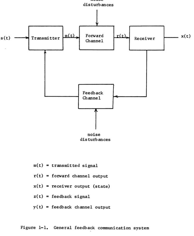
In Figure 1-1 a block diagram of a general feedback communication system is shown. The information to be conveyed over the forward channel can take any form (digital or analog) depending on the application. For example, the channel might be used to transmit a single bit in T seconds, 20 bits in T seconds, a single bit sequentially, the value of a random variable, or a segment of a
noise disturbances
noise disturbances
- transmitted signal
= forward channel output
= receiver output (state)
= feedback signal
= feedback channel output
Figure 1-1. General feedback communication system
s(t)
x(t)m(t)
r(t) x(t) z(t) y(t)random process. At the transmitter the signal s(t) which contains the message is combined with the feedback signal y(t) to generate the transmitted signal m(t). The forward channel could be an additive white noise channel or could contain more complicated disturbances; the results of this thesis are concerned primarily with a white noise forward channel.
The output of the forward channel r(t) is the input to the receiver. The receiver attempts to recover the message from the observed r(t) and also generates the return signal z(t), the input to the feedback channel. The feedback signal z(t) is corrupted by the feedback channel disturbances which could be additive noise, delay, or other types of interference. In many cases this feedback channel will be assumed to be noise-less and without delay. In other words y(t) = z(t).
Typically there are realistic constraints imposed on the system structure or system signals. The transmitted signal m(t) must have a power (peak and/or average) constraint and similarly for z(t) if the feedback channel is noisy. Trans-mitted signal bandwidth constraints might also be imposed. Given the necessary system constraints, the system must be
designed to maximize the overall performance whether the criter-ion be probability of error for digital systems or mean square error for analog systems.
Although the signals shown in Figure 1-1 are functions of the continuous variable time, most authors who have studied feedback systems previously have studied discrete-time forms of the continuous-time system of Figure 1-1. For the
discrete-time version the transmitted signal m(t) becomes m (a function of the integer k) where k represents the k-th sample in time or the k-th coordinate of some other expansion. Depending on the expansion employed, such discrete systems may or may not be easily implemented in practice. Even from an analytical point of view such discrete formulations are not always tract-able. The analytical comparison of the two analysis procedures is the difference between sums and integrals, difference equations and differential equations. This thesis will treat
continuous-time systems except for the following discussion of previous investigations. Most authors subsequently apply their discrete results to continuous-time systems; hence, by always dealing
with continuous-time signals such limiting procedures are avoided.
1.2 Summary of Previous Study of Feedback Communications One of the earliest summaries of feedback communications systems is given by Green [1]. Besides discussing some practical applications of the use of feedback, Green includes a paper by Elias [2] which describes a pre-decision feedback system. Elias describes a system which is able to transmit at the channel capacity of a white noise channel of bandwidth W = k W (W = source
width, k = integer) by utilizing a noiseless feedback channel of the same bandwidth. Shannon [5] has shown that even the availability of noiseless feedback does not alter the ultimate error-free transmission rate of the forward channel; hence, throughout this thesis feedback will never improve the ultimate rate of channel capacity, but perhaps make operation at rates approaching capacity easier to achieve.
Elias achieves channel capacity by breaking utp the wide-band channel into k separate channels interconnected with k-l noiseless feedback channels. For Elias operating at channel capacity implies that the suitably defined output signal-to-noise ratio is at the maximum value prescribed by channel
capacity. Such a system is said to achieve the rate-distortion bound on mean square error for analog systems although Elias omits reference to the rate-distortion bound. Elias [3] has extended his work to networks of Gaussian channels.
Schalkwijk and Kailath [4] have adapted a stochastic
approximation procedure to form a noiseless feedback scheme which can operate at error-free rates up to the ultimate rate given by the forward channel capacity. In their system a message space is defined and a probability of error (Pe) calculated. For message
e
rates less than channel capacity Pe tends to 0 in the limit as the number of messages and the length of the signalling interval increase. Such behavior is usually what is meant when a digital
Schalkwijk and Kailath consider a discrete time system operating over a T second interval with TN seconds between samples. The
message alphabet of M signals consists of M equally spaced numbers e. in the interval [-.5,.5]. The receiver decodes the received signal after T seconds to the 0I which is closest to the final value of the receiver output x. The receiver output x is
fed-back to the transmitter at each time instant over the noiseless feedback channel. The transmitter attempts to drive the receiver output state xk to the desired message point (a particular member of the M ei.'s) by transmitting at the k-th instant
1
mk = (Xk - 0) (1.1)
The assumed receiver structure is linear and satisfies the difference equation
X
1(M + nx
= 0
(1.2)
Xk+l
=
x
k-
kk
=n)
where
= constant
nk = additive noise at k-th time instant
E[nknj] = N/2 6kj
The constants and N are adjusted so that the average power constraint
N
P 1 [ 2 (x -) 2 ] (1.3)
ave T iO i
holds and P is minimized.
The performance of this system is shown to have a P which
e
tends to 0 at information rates less than
C = P ave/N nats/sec (1.4)
ave o
as T, , and N all go to infinity in a prescribed manner. C is
the channel capacity for the infinite bandwidth forward channel with or without feedback. The information rate R. in nats/sec is
defined as
1
R = In (M) (1.5)
For finite values of T, M, and N Schalkwijk and Kailath's system gives a lower P than that obtained for block coding
e
(without feedback). In other words even though both systems have a P which approaches 0, the feedback scheme approaches 0 much more
e
rapidly. The feedback system is also structurally simpler and
does not involve complex coding-decoding algorithms for the messages. Schalkwijk [6] in a companion paper shows how to modify the wideband scheme for use over bandlimited channels. A bandlimited channel for bandwidth W implies that (for the above scheme)
C
N 2 T (1.6)
C
and that a (in Equation 1.2) becomes a function of k (time). The modified system then achieves error-free transmission (in the limit)
at rates u to the bandlimited channel capacity
P
CW = W ln(l + ave (1.7)
c NW
An important assumption of'these two papers is noiseless feedback. In a practical situation there always exists some noise in any system. Both of the above papers calculate the performance of the feedback systems if noise is inserted. The performance exhibits a sharp threshold at the point where the feedback noise dominates the overall system performance. No matter how small the feedback noise is (relative to the forward channel noise), eventually P tends to 1 as M, N, and T tend
e
to infinity. The conclusion is that the feedback systems described by Schalkwijk and Kailath cannot achieve channel capacity if
the slightest amount of feedback noise is present. In a practical situation where P need not be 0 the feedback noise might or
e
might not be small enough for satisfactory operation of the feed-back system. No attempt was made by Schalkwijk and Kailath to take into account in system design possible feedback noise.
Omura [7,8] considers the identical discrete-time problem from a different viewpoint. Assuming an arbitrary one-state recursive filter at the receiver, Omura proceeds to determine the best transmitted signal for that receiver (given the receiver
state is fedback) and then to optimize over the arbitrary one-state filter. His arbitrary filter is described by
Xk+l Xk + kXk gk (k + nk)
(1.8)
xo=0
where {k } and {gk} are free parameters to be determined. mk is the transmitted signal which depends on the noiseless feedback signal xk-1 and the message point ; the exact dependence of the transmitted signal on these two inputs is optimally determined. The optimization for {mk}, {k }, and {gk} can be formulated using dynamic programming and then solved.
The optimal transmitter structure is linear (of the same form as Equation 1.1). For any arbitrary set {k} the optimization yields a particular set {gk} such that all of these systems have identical performance. Omura's system differs slightly from Schalkwijk and Kailath's in that Omura's has a constant average power
E[mk = (Omura) (1.9)
ave
whereas Schalkwijk and Kailath have a time-varying instantaneous average power
V
d2] 1 (Schalkwijk) (1.10)
E[mk2 I
Both, of course, satisfy the average power constraint Equation 1.3, but in different ways. Both systems have similar (but not identical) performance; Omura's performs better for finite T, , and N.
Turin 9,10] and Horstein [11] consider a different system utilizing feedback. They are concerned with transmitting a single bit (or equivalently one of two hypotheses) sequentially or
non-sequentially. Thus far only nonsequential systems have been mentioned. The receiver of the sequential system computes the likelihood ratio
of the two hypotheses, H+ and H ; the ratio is also fedback to the
transmitter over a noiseless feedback link. For sequential operation the system is allowed to continue until the likelihood ratio at the output of the receiver reaches one of the two
thresholds, Y+ and Y. The time required for each bit to be determined at the receiver will fluctuate, necessitating some data storage capabilities. If the system is operated nonsequen-tially, the receiver chooses the most likely hypothesis at the end of the fixed transmission interval.
For Turin and Horstein the receiver (likelihood ratio computer) is fixed and the optimal transmitted signal to be determined. In particular they require the transmitted signal to be of the form
m+(x,t) = ± U (x)a(t) (1.11)
where x = likelihood ratio receiver output.
The signal transmitted under either hypothesis is the product of a time function a(t) and a weighting U(x) due to the current state of the receiver. A peak-to-average power ratio is defined
a= Ppeak /P (1.12)
peak ave
and a peak power constraint is applied by varying . Turin considers
a=l and a>-log2(Pe) = a'. Horstein considers the remaining values
of a.
For a tending to infinity (i.e., no peak power constraint) the sequential system can operate up to an average error-free rate
given by channel capacity. For a given (nonzero) P and average
e
time/decision T the sequential system has an average power advantage of
= -log2(Pe) (1.13)
over the same system without feedback. Such a system without feedback would be equivalent to a nonsequential matched-filter likelihood ratio computer at the receiver.
For a finite peak power constraint it is impossible to operate the system at any nonzero rate with P =0. Without allowing an
e
infinite peak power neither Turin and Horstein nor Schalkwijk and Kailath can achieve channel capacity; Omura's scheme, however, does not require an infinite peak power.
Kashyap [21] has considered a system similar to Schalkwijk and Kailath't
s, but with noise in the feedback channel. Kashyap's result is that nonzero error-free information rates are possible for rates less than some R <C. Unfortunately his technique requires
c
an increasing average power in the feedback channel as T, M, and N increase. Basically the transmitted power in the feedback signal is allowed to become infinite so that the feedback link is really noiseless in the limit and nonzero rates can be achieved. That he could only achieve a rate R <C must be attributed to
c
his not letting the feedback channel power get large enough fast enough.
Kramer [22] has adapted feedback to an orthogonal signalling system. Orthogonal signalling systems (unlike the linear signalling systems treated thus far) will operate at rates up to channel
capacity without errors without feedback. The addition of feed-back cannot improve on this error-free rate, but it does improve
on P for finite T, M, and N. In fact it is not surprising
e
that orthogonal signalling with feedback is much superior to linear signalling with feedback. Of course, the orthogonal system would be somewhat more complex in terms of transmitter-receiver implementation. For the most part this thesis is not concerned with the addition of feedback to already complex systems; the main advantage of feedback appears to be a saving in complexity at the expense of a feedback channel. However, for some channels (e.g., fading) orthogonal signalling is almost a necessity for satisfactory performance.
Kramer also considers noisy feedback, but like Kashyap, lets the feedback channel power approach infinity so that the noise in the feedback link "disappears" allowing capacity to be achieved in the same manner as his noiseless system.
Butman [23,24] has formulated the general linear feedback problem similar to Omura's. Butman assumes a linear transmitter as well as receiver and optimizes over these two linear filters; here a linear receiver is assumed (as with Omura) and the optimal transmitter is shown to be linear. For noiseless feedback Butman's discrete-time system performs better than Omura's, but Omura's
system can be made equivalent to Butman's in performance by removing some of Omura's approximations. For noisy feedback Butman-has
some results for suboptimal systems; analytic solution for the optimal system seems impossible. Unfortunately his partial results
cannot be extended to the continuous-time systems treated in this thesis. Butman, however, did impose a finite average power
constraint on the feedback transmitter and thereby formulated a realistic problem of interest which others have failed to do.
1.3 Outline of Thesis
In the remainder of this thesis noiseless and noisy feedback systems are studied employing a continuous-time formulation of the problem. The primary concern is not so much with achieving capacity of the forward channel, but with minimizing either the probability of error (P ) or the mean square error for finite time
e
problems.
Chapter 2 treats the continuous version of Omura's problem with noiseless feedback. Also investigated are the physical characteristics (peak power, bandwidth, etc.) of such noiseless feedback systems.
Chapter 3 treats the topic of analog signalling over noise-less feedback systems. This is a new application of feedback and has not been studied before.
Chapter 4 treats the digital problem in Chapter 2 when there is noise in the feedback link. The results are primarily approximate since analytic solution seems impossible. Nevertheless, such
partial results are most useful in systems engineering since the optimal systems (if they could be determined) appear to be not much better than some of the sub-optimum systems studied. Noiseless feedback systems turn out to be very sensitive to the noiseless assumption: noiseless feedback can be viewed almost as a singular
-22-system achieving dramatic performance improvement. The addition of noise in the feedback link which makes the sstem more
realistic also cuts down the performance improvement.
Chapter 5 deals with extensions of this work and suggestions for future study.
Chapter 6 contains some results unrelated to feedback systems. They are included for completeness since the results were obtained during my graduate research.
Noiseless Feedback -- Digital
In this chapter a noiseless feedback system will be developed and its performance calculated. The system development is
similar to that of Omura [7,8], but the analysis is in terms of a continuous-time variable t instead of a discrete variable k. The mathematics necessary for this formulation involves stochastic differential equations, dynamic programming, and stochastic optimal control theory. No attempt will be made to prove the necessary results from these areas; the reader is directed to the references for further information.
2.1 Definition of Noiseless Feedback System
The receiver structure is assumed to be a simple linear system described by a first order differential equation. The motivation for such a receiver structure is primarily the
simplicity and practicality; the prospect of actually having to build the system if it will work satisfactorily is not an
unpleasant one. Also, under the Gaussian noise assumption the linear system will turn out to be optimal.
The receiver (by assumption) is an arbitrary one-state
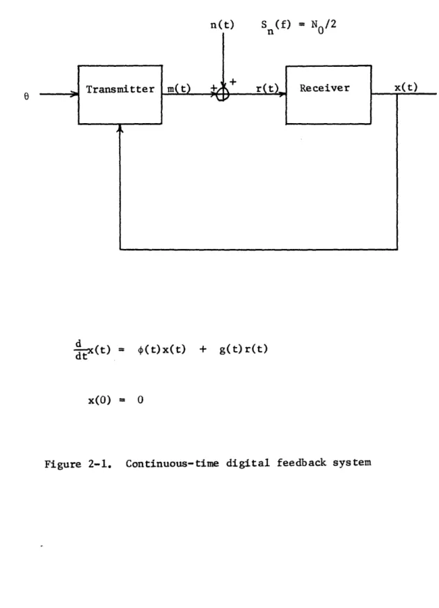
linear filter operating on the received signal r(t) in the interval O<t<T. The state equation is
d_ x(t) = (t) x(t) + g(t) r(t) (2.1)
dt
-23-where (t) and g(t) are to e selected in an optimal manner.
A more general linear receiver would be one of higher dimensional state, but the analysis for the one-state system indicates that extra states in the receiver will not improve the system perform-mance; hence, the assumption of a one state receiver does not reduce the ultimate system performance.
The forward channel is an additive Gaussian white noise channel as indicated in Figure 2-1. The feedback channel is noiseless and allows the transmitter to know the state, x(t), of
the receiver.
The digital signalling problem consists of transmitting one of M equiprobable messages from the transmitter to the receiver with a minimum probability of error. Assume that the M messages are mapped to M equally spaced points in the unit interval
i-l
[-.5,.5]. The random variable takes on the value -. 5 + (i=1,M) depending on which message is transmitted. For this system of coding the transmitter conveys the value of a random variable which can be mapped back to the actual message if desired.
The performance criterion for the system is the probability of error (Pe), and ideally this criterion is to be minimized. Unfortunately this criterion is not tractable for selecting the best transmitter structure minimizing P . Instead a quadratic
e
criterion is used to optimally select the transmitter structure; the system is designed to minimize the mean square error in
n(t)
S (f) = Nn/2
d
dx(t)
=
~(t)x(t) + g(t)r(t)
x(O) =
Figure 2-1.
Continuous-time digital
feedback system
Several comments about this criterion are appropriate. If the transmitter is assumed linear, forming the minimum variance estimate of at the receiver (and decoding to the nearest message point) is equivalent to minimizing Pe ; hence, the solution
obtained shortly is the minimum P system when the transmitter
e
is constrained to be linear. As will be shown, the best trans-mitter structure for minimizing the quadratic criterion is
linear anyway. In Chapter 3 analog estimation problems are treated; for these problems the criterion is truly a mean square error one so that the results of this chapter are directly applicable.
Besides the message point , the transmitter has available x(t), the current state of the receiver. This information is
transmitted continuously back to the transmitter over the noise-less (and delaynoise-less) feedback link. Knowledge of the state x(t) is sufficient to specify completely all characteristics of the operation of the receiver; hence, any other information
supplied over the feedback channel would be redundant. Actually the transmitter also has available the past values of x(t)
(i.e., x(T) for O<_T<t), but these values turn out to be
un-necessary. The general structure of the transmitter is arbitrary with m(t) = f(e,x(t),t); the optimization implies that f( , , ) is actually linear in the first two arguments.
In the formulation the functions (t) and g(t) which
determine the receiver are completely free. In a practical system one or both of these functions might already be specified as part
of the system or by cost considerations. Here these two
functions will be assumed unconstrained.
If the receiver state at t=T is to be the minimum mean
square error estimate of , the quadratic criterion to be
minimized is
2 2
a = E[ (x(T)-O) ] = minimum (2.2)
with the expectation over the forward channel noise and over
O (the message space).
One further constraint remains, that of transmitted power or energy. The transmitted signal m(t) is unspecified, but
it must satisfy
T 2
f dt E[m (t)] < 0 = P Tave (2.3)
0- ave
0
as an appropriate transmitter energy constraint. The expectation is over the channel noise and the message space. A constraint on the feedback channel energy has no meaning when the channel
is noiseless.
The constraint in Euation 2.3 is only on the average
energy used. During any particular T second interval the actual energy used can be more or less than the average EO. Thus,
the transmitter must be able to exceed a transmitted energy of E in T seconds frequently. The average over many intervals
0
(messages), however, is E0.
Summarizing the problem just formulated, the performance
2.
a in Equation 2.2 is to be minimized subject to the energy constraint in Equation 2.3. The minimization is over the trans-mitter structure m(t) and the free receiver functions (t) and
g(t).
2.2 Stochastic Optimal Control and Dynamic Programming: Formulation Having specified the problem in the previous section,
the solution technique follows by relating the problem to the work of Kushner [12,13]. First of all, some interpretation must be given to systems specified by differential equations with a white noise driving term as in Equation 2.1. Such
stochastic differential equations are subject to interpretation according to how one evaluates the limiting forms of difference equations. The two principle interpretations are those of Ito [18] and Stratonovich [19]; the only difference between
the two is the meaning of white noise. For this problem, though, the two interpretations are equivalent since the differential equations are linear.
Kushner [12,13] using the Ito interpretation has formulated the stochastic optimal control problem in dynamic programming. Technically Ito differential equations need to be expressed in terms of differentials rather than derivations; throughout this thesis derivative notation will be used for simplicity. Continuing with Kushner's formulation, let the stochastic system to be
controlled by specified by a nonlinear vector state equation
d
x = f(xut) + (t)(2.4)
where (t) is vector white noise with covariance matrix
For the communications problem here the state equation is Equation 2.1 or
dt x(t) = (t) x(t) + g(t)[m(t) + n(t)] (2.6)
The white noise i(t) in Equation 2.4 corresponds to g(t)n(t) in Equation 2.6, the covariance function of the latter being
N
0 2
E[g(t)n(t)g(u)n(u)] = g (t) 6(t-u) (2.7)
The ptimal control problem for Kushner is to determine the control u within some control set in the interval of operation [,T] which minimizes the cost functional
T
J = E[f dt L(x,u) + K(x(T))
1
(2.8)0
which contains an integral cost plus a terminal cost. The
notation E[ is the expectation conditioned on all the inform-ation which is available to the controller u. The control
variables in the feedback communication problem are m(t),
¢(t), and g(t). (t) and g(t) are simply functions of time, but m(t) is more complicated because it can depend on the feedback
signal x(t). The solution proceeds first by determining m(t) (the transmitter structure); then the problem is no longer stochastic control and (t) and g(t) can be found by ordinary means. Therefore, identifying Kushner's control u with m(t),
within the control set -<m(t)<- in the interval [n,T] wrhich
minimizes
T
J = E[ X f dt m (t) + (x(T)-O- ] (2.9)
0
The constant X is a Lagrange multiplier necessary to impose the average energy constraint in Equation 2.3.
This optimal control problem of Kushner differs from the ordinary (deterministic) optimal control problem by the white noise term in the state equation and the exDectation E[ .
Deterministic optimal control can be treated by dynamic programming techniques of other techniques derived from Pontryagin [25];
stochastic optimal control cannot be formulated with Pontryagin's method due to the nondeterministic nature of the system state equation.
For the above stochastic problem dynamic programming defines an optimal value cost function
T
V(x,t) = min E [ f dt (x,u) + K(x(T)) ] (2.10)
t
V(x,t) is the minimum cost of starting in state x at time t
and proceeding to the end of the interval. Kushner [12]
shows that the function V(x,t) must satisfy the partial differ-ential equation
0 = min E*{ aX + <V, f> + L(x,u)
~t
DX'-u£
+ Tr[S(t) -- ]} (2.11)
where ordinary matrix notation has been employed to simplify the equation. The boundary condition for the partial differ-ential equation is
V(x,T) = K(x(T)) (2.12)
The solution of Equation 2.11 for V(x,t) and u is not easy. No general techniques are known for solving such systems just as similar techniques are not available for deterministic control problems.
Proceeding with the parallel development of the communic-ations problem, define the cost functional
T 2 2
V(x,t) = min E[ f dt m (t) + (x(T)-0)2 ] (2.13)
m(t) t
It follows from above that V(x,t) satisfies
0 = min E* { V + av [(t)x(t)(t)+gt)m(t)]
m(t)
2 N02 a2v
+
X
m(t) +
-g
(t)
} (2.14) axsubject to the boundary condition
V(x,T) = (x-e)2 (2.15)
Note that the quantity of interest (J in Equation 2.9) is
Observe that although the control m(t) is written with
only a time argument, the control is actually a function of
t, x(t), and . This will become apparent when E*[ ] is evaluated. Also Equation 2.15 implies that 0 is fixed and known. Later the results will be averaged over to obtain
the system performance.
2.3 Solution of Noiseless Feedback System
In this section the solution to the stochastic optimal
control problem will be found to determine the dependence
of m(t) on x(t) and 0. Following this, the functions (t) and
g(t) will be optimized to complete the system.
The conditional expectation E[ ] is conditioned on the fact that the transmitter knows x(t); hence, E[x] = x. Inserting this fact in Equation 2.14 allows E[ ] to be evaluated, leaving ~V ~V = min { + x[(t)x(t)+g(t)m(t) + m2(t)
m(t)
N
2
N0 2 - } (2.16) +-g (t) 2 4 ~The minimization over m(t) is just a minimization of a quadratic form in m(t) (for a fixed t). Evaluating Equation 2.16 at its minimum gives
2 2
0 = t - g (t) -2 2W
.L
+ x ~(t)x(t) (2.17)where the minimizing choice of m(t) is
m(t) = _g(t) [;V (2.18)
Equation 2.18 expresses m(t) in terms of the as yet unknown V(x,t).
Several comments can be made at this point relating stochastic optimal control and deterministic optimal control. In this problem the optimal control m(t) is not affected directly by the noise term in Equation 2.16, namely,
2 2 2
(N0/4)g (t);2V/Bx is independent of m(t). Thus, the solution for m = m(x,t) is the same as would be obtained with no noise present; this problem corresponds to optimal control of linear
systems treated similarly in Athans and Falb [14]. In general the addition of the noise term in Equation 2.15 is the only difference in the dynamic programming formulation of stochastic problems. For many problems the solution to the deterministic problem will also be the solution to the stochastic problem
if the control is given as a function of the state, not just
a function of time. The techniques of Pontryagin are not applicable to stochastic problems since they do not explicitly obtain the control as a function of state.
Returning to the partial differential equation for V(x,t) in Equation 2.17, the solution is not at all obvious for this or most other partial differential systems. -Since there is a
-34-quadratic cost imbedded in the problem, it is perhaps not unreasonable to expect that V(x,t) is also a uadratic form.
Therefore, try a solution of the form
9
V(x,t) = P(t) [x- y(t)] - + r(t) (2.19)
where P(t), y(t), and r(t) need to be determined. Inserting
the above expression for V(x,t) into Equation 2.17 and equating
2) 0
the coefficients in front of x , x, and x to zero, there
result differential equations which P(t), y(t), and r(t) must satisfy if V(x,t) in Equation 2.19 is to be the solution. The differential equations and boundary conditions for these three functions are
2 2
d 2 (t)p2 (t
d d P(t) P(t) = (t)P (t) - 2p(t)P(t) P(T) = 1 (2.20)
d- y(t) = t)y(t) y(T) = (2.21)
d N
0 2
d r(t) = - No g (t)P(t) r(T) = 0 (2.22)
By solving these three equations, V(x,t) is determined by Equation 2.19, implying that m(t) is (from Equation 2.18)
m(t) - g((t) (x(t) - (t) (2.23)
which is the desired optimal transmitter structure. Observe
that Equations 2.20-22 are easily solved numerically by integrating backwards from tT where the boundary conditions are given.
Actually in this problem the equations can be integrated analytically. Starting with Equation 2.21, define
t
P(t,T) = exp[ f dv (v)] (2.24)
T
as the transition function of Equation 2.21. Applying the
boundary condition on y(t) gives
0
y(t) = 0 (t,T) = ~(Tt) (2.25)
as the solution for y(t) in the interval. y(t) represents a
type of tracking function for the transmitter; whenever x(t) (the feedback signal) happens to equal y(t), the transmitted signal m(t) is zero. y(t) is that value of x which will cause
the receiver to "relax" to x(T) = 0 with no further input
starting at state x = y(t) at time t. The additive channel
noise will always disturb the receiver state so that the trans-mitted signal will never be zero for any measurable length of
time.
Equation 2.20 is a Ricatti equation for P(t) (without a
driving term). The solution can be written
2
P(t) = (T,t) (2.26)
1 T 2 2
1 + f dT g (T)D (T,T) t
by employing the boundary condition. Finally the solution of Equation (2.22) yields
-36-N0 2
r(t) =- X ln[P(t)D (t,T)] (2.27)
Now that V(x,t) has been determined the initial point V(0,0) can be evaluated to give the original functional as
T 2 2
V(0,0) = min E*{ f dt m (t) + (x(T)-e)
m(t) 0 = P(0)y(O)2 + r(0) N = es- . 2 A ln(s0) (2.28) where s is defined as sO - P(0) 2 (0,T) (2.29)
The overall minimum cost (minimum over the transmitter structure only is only a function of
T 2 2
+
f
dT g (T)' (T,T) (2.30)~0
and N/2, , and . Recall that is assumed known until the average over e is taken later.
The next step in the optimization is to determine g(t) and ¢(t) by minimizing the cost in Equation 2.28 over all possible g(t) and (t). Assuming no constraints on these functions, from Equation 2.30 g(t) and (t) (or equivalently (T,t)) enter together
in the cost. Therefore, either g(t) or (T,t) can be set to
1 without any loss in generality. Set tD(T,t) = 1 (which
implies (t) = 0) as the choice leaving the above equation
as
T
L
1+1
fdT
g(T)
(2.31)
so
0 0Setting (t) = 0 implies that the receiver structure is only a
multiplication (or correlation) of the received signal by g(t) and integration of the product; the arbitrary memory allowed origina±lly is not needea. qulva±ently trhe multiplicative function could be set to unity and the receiver structure would only involve the memory term (t). Also one could keep both
g(t) and (t) if, say, (t) is a given fixed part of the receiver.
All of these variations of the receiver have the same overall performance if their values of s in Equation 2.30 are identical.
If a higher state receiver had been assumed initially, the unnecessary redundancy of the extra states would appear at this
point in the analysis.
Reverting to ¢(t) = 0 and s given by Equation 2.31, V(0,0) is still a functional of the arbitrary function g(t). The optimal g(t) can be found by ordinary calculus of variations. Perturbing Equation 2.28 gives
2 0
0 =V(O,O) = [e- - 2s ] 6s (2.32)
s
0The right hand side is zero if
s
0= 0 or if the bracketed term
is 0. 6s = 0 implies that g(t) = 0 which is an impossible
-38-solution; therefore; setting the bracketed term to 0 implies
N X N0 s = (2.33) 2 2e or T 2
f
d g (t) 2 = X = constant (2.34) 0 T Nwhich is the only restriction on the optimal g(t). Note that no solution for g(t) came out of the perturbation, only the above constraint on the integrated square of g(t). This singular solution implies that there are an infinite number of possibil-ities for g(t), all of which have some performance as long as Equation 2.34 holds.
At this point there are still several steps remaining to obtain the overall system structure. The multiplier needs to be determined such that the average transmitted energy is Eo0. This averaging involves averaging over also. However, the
transmitter structure has been determined as
m(t)
MW
= - g(t)P(t)%
(x(t)WO
- )(
(2.35)(23)
where P(t) is known (Equation 2.26), X is an unknown constant to be determined, and g(t) s (almost) arbitrary. The transmitter
sends a multiple of the instantaneous error between the receiver state x(t) and the desired state .
2.4 Evaluation of the Performance of Feedback System
feedback problem in terms of te (almost) arbitrary g(t)
and the constants X and . Frequently in optimization
problems the solution for the optimum is relatively straight-forward, but the actual evaluation of the performance is more difficult; this problem is no exception.
Using the optimal transmitter structure in Equation 2.35, the state equation of the overall system (Equation 2.6)
2
d _ g (t)P(t) (x(t) - 0) + g(t)n(t) (2.36)
x(O) = 0
for (t) = 0. Define the instantaneous error given 0 as
2
K(t) - E[(x(t)-0)2 ] (2.37)
The differential equation for K(t) is
NO
dK(t) 2(t)P (t) + (t) (2.38)
K(0) = 2
Therefore, the conditional performance (mean square error) of
the feedback system is the final value of K(t), namely
-40-To relate this performance to the energy used, define
it
E0(t) - f dT E[m (T)1 (2.40)
0 0
as the energy used after t seconds. In differential equation form
2 2
d g(P K(t)= (t)2.41)
dt E
0E0(0) = 0
The remaining differential equation to specify the performance calculation is that for P(t) given in Equation 2.20 (for
4(t)=0). In order to have all boundary conditions at t=0, integrating backwards in Equation 2.20 gives
0
P(0) = s = (2.42)
() 22
2e2
Solution of the three equations for K(t), E(t), and P(t) can take many forms. Since g(t) is arbitrary except for the integral square constraint in Euation 2.34, a fixed g(t) could be selected and the equations integrated numerically or
analy-tically. For this problem analytical integration of these
equations for an arbitrary g(t) is possible; this procedure
was the original solution technique.
In view of the answer obtained, the following derivation
-41-2
a fixed known 0. ultiplying Equation 2.38 by P (t) and rearranging terms yields
dK 2 3(t) N 2 2
dt P (t) +
2
(P
(t)
(2.43)Inserting the expression for dP/dt gives
N
dt (2.44)
Integrating and using the initial conditions implies
K(t)P2 (t) = 2 X P(t) (2.45)
which further implies that Equation 2.41 can be written
d NC 1 d
d-
E0K(t)
- K(t)
(2.46)Now the energy and performance are directly related; integrating gives
K(t) = exp[-2En(t)/NC]
If is chosen properly, then E(T) = E and
2 = 62 exp[-2E0/N0]
lo
(2.47)
as the conditional performance in terms of the allowed energy. The absolute performance is obtained by averaging over 0
(the message space) to give the value of the minimum of
Equation 2.2 as
2 2
O = E[ ] exp[-2E0/N 0 (2.49)
Unfortunately the solution leading to Equation 2.40 does not contain some of the details of the system structure, such
as the value of X and the constraint on g(t). The most direct
(although cumbersome) way to obtain the value of is to integrate Equation 2.41, equate E(T) to E0, and evaluate
as
2 2
2 E[
2
]
=2
E[E
2
]
% 2 N0 exp[-2E0/N] = 2 No (2.50)
which implies the only constraint on g(t) is
T 2 2 E[62
f dt g (t) = (1 - exp[-2E 0/N0]) (2.51)
0 NO
Observe that the parameter which was defined in Equation 2.29 is te fractional mean square error (or normalized mean souare error)
2 .,~~~~~~~~~~~~~~~~~~C
2 sO = exp[-2E0/N0] (2.52)
The performance in Equation 2.52 is the fractional mean square error for estimating any random variable 0 since the robabilitv
density of has not entered the analysis. Implicitly 0 has a zero mean and a finite variance.
2.5 Probability of Error for Linear Coding of Messages In Section 2.1 the mapping from the message space (M equiprobable messages) to the random variable was outlined. Here this mapping will be used to calculate the probability of error (Pe) for the digital signalling scheme.
The receiver decodes the terminal state x(T) into which-ever message is most probable. For M equiprobable messages
the output space for x(T) (the values X(T) may take) can be broken into uniform width cells (except for the end cells near .5) corresponding to the M possible messages. If x(T) falls into the i-th cell, i is the most probable value
of and the i-th message is the most probable message.
Assume that a particular 8. is sent. The probability of
1
error given 0. sent is approximately the average (over all
1
messages) P of the whole system; the only difference is that
e
the endpoint messages Oi + .5 have slightly lower conditional
probability of error. Henceforth, this conditional P given
e
8i sent will be treated as the average P for the system; it is
i e
negligibly higher than the true average P.
e
For a particular 0. if n(t) is Gaussian, then x(T) is a
1
Gaussian random variable. From the previous section given
i then
E(x(T)-0i) ] 8ei so i exp[-2E0/No] (2.53)
By appropriate manipulation of the system differential equations
the mean value of the difference is
E[(x(T)-ei)] = -
e
(2.54).~~~~~~~~~~
0
which implies that x(T) is a biased estimate of 0i . Combining
ig
the above two equations gives the variance of the Gaussian random variable x(T) as
!~~~~~~~~~~
Var[x(T)1 Vat ] = ei s( - s) (2.55)
[(!
:1
On the average the variance is
22
Var[x(T)] = E[0 ] s0(l - so) 1 (2.56)
Although the Var[x(T)] really is not the same for each i, for purposes of analysis it will be assumed to be the constant
2 2
C above. Another approach would be to upper bound Oi by its
maximum value of .25 to remove the i dependence. The resulting P would be an upper bound not significantly different from P
e e
calculated using 2l.
The transmitter message space [-.5,.5] is compressed by
a bias factor (1 - s) at the receiver; thus, whereas the
message points are /(M-l) apart at the transmitter, they are only (-s 0)/(M-1) apart in the receiver space. If 0. is
1
(l-s0 )( i 0 i -2(M-1)' 2(M-1l)) < <i x(T) < ( + 2(M-))(1-S )
2
(M-
1) (lo
(257
(2.57) The probability of error is the probability of exceeding theabove cell and can be written
P = P - 2 e e
i
f
1-s0 2M-2 dz exp[-z2/2ao] 0o Q(v) = f dz 1 exp[-z2/2] V 7~-2 7 P becomes e P = 2 Q( e 1 2I( _ 1)l/2 2(M-l) E8A 2] ° or using Equation 2.52 1 2(M-1) E0I
(exp[2Eo/N0] - 1)1/2) (2.61)If the variance E[0 ] is approximated by the variance of a
random variable with uniform density in the interval [-.5,.5], then E[02] =1/12 and P can be evaluated. A better choice for E ]
e
would be the actual variance of 0 for the message space assumed; this is done in the next section.
Defining (2.58) (2.59) (2.60) P = 2 Q( e I I i I 1i Iii i I I i i i I i I II I i i .i I
-1
-A comparison of P above with that obtained b Omura shows
e
that Omura assumes E[02 ] = 1/12 and that, if the bias (-s)
can be ignored, his discrete system has the same P when
e
evaluated in the continuous-time limit. The bias can only be ignored for large signal-to-noise ratios (2E/N ); mura
j 0
fails to note this fact.
Schalkwijk and Kailath's system output is an unbiased estimate of (by their arbitrary choice) and has no such restrictions. Their performance, however, is inferior in the limit. If Schalkwijk and Kailath allowed a biased estimate to be fedback and optimized their system, better performance could be obtained. Recall, however, that they make no optimiz-ation attempts in their applicoptimiz-ation of a stochastic approximoptimiz-ation theorem.
As noted by Omura, Schalkwijk, and Kailath, P goes to
e
zero in a doubly exponential manner for feedback systems. To relate this P to channel capacity, using Equations 1.4 and
e
1.5 to define capacity and rate, the probability of error is (approximately)
i
2]-1/2
P = 2 Q( E exp[(C-R)T] ) (2.62)
e
which is Omura's result for unbiased artitioning (P when the
e
bias is ignored). A nofeedback system employing block orthogonal coding also has a P which goes to zero (for increasing T and
and R<C), but the error is only singly exponential in T. The doubly exponential dependence of the feedback systems implies that for finite T the feedback system will have a lower P than the block orthogonal system without feedback.
e
Schalkwijk and Kailath [4] have some curves which indicate the improvement of the feedback system over the block ortho-gonal system.
As noted earlier, Schalkwijk and Kailath do not use a biased system. From their paper the P obtained by them is
e
P = 2(½ E[02]-1/2 exp[(C-R)T] .454 )(2.63)
e2
which is different from Equation (2.62) by the factor .454. For finite T their system will perform substantially worse
than the feedback scheme of this chapter. For example, if
e
the continuous-time feedback system has an error P = 101, -2
the unbiased system (Equation 2.63) would have Pe = 10 for
e
the same C, T, and R. This difference is a consequence of
the fact that feedback signal of Schalkwijk and Kailath is an unbiased estimate of .
2.6 Comparison of Feedback System Performance with Butman's Results Butman [23] assumes a general linear receiver and linear
transmitter for the discrete-time feedback problem. His solution for the optimal linear system has the same limiting (discrete to
continuous) performance as Equation 2.61. This result is further verification of the fact that the simple one-state receiver
assumed in this chapter performs as well as any higher dimensional arbitrary linear receiver.
To rewrite Equation 2.61 so that it conforms to Butman's result requires only the evaluation of E[0 2 ]. For the random variable as described in Section 2.1, the variance is
E[] 12(M-) (2.64)
12(M-1)
which for large M is 1/12. Inserting the above expression for E[e2] into Equation 2.61 gives
3(exp[2E0/N0] - 1) 1/2
P 2 Q([ 2 ] ) (2.65)
e
M - 1
which is Butman's result in the continuous-time limit.
2.7 Performance of Linear Receiver without Feedback
Some idea of the advantage and improvement of the feedback system can be gained by examining the same problem without the feedback link. Given a linear receiver, energy constraint, and cost function (Equation 2.13), determine the best transmitter
structure and optimal receiver parameters for minimizing the
cost. The solution follows using ordinary calculus of variations. The best transmitter structure is linear in , that is,
where h(t) is arbitrary except for energy normalization. The linear receiver is "matched" to the waveform li(t). Rather than demonstrate the approach just outlined for obtaining the solution to the nofeedback problem, the preceding results of the noiseless feedback system can be extended to the nofeed-back problem, the preceding results of the noiseless feednofeed-back system can be extended to the nofeedback system.
The solution assuming no feedback implies that F,[ ] is a different conditional expectation. E*[ ] is conditional on the information available at the transmitter; now, without a feedback channel, there are no conditions, namely
E*[x(t)] = x(t) = mean of x(t) (2.67)
replaces the previous definition of E*( ]. Equation 2.16 now becomes
0 = min {E*[aV] + g(t)m(t) E[aV] + ¢(t) E*[x(t) x3V]
m(t)
at~N
ax
axv
N
+ Xm2(t) +4 g (t) *
g (t)
a 2 (2.68)~ax
2The minimization over m(t) roceeds as before giving
m(t) = g(t) E*[V (2.69)
I~~~~~~~~~~~~~
0
E*3V ) E*2v + (t) E*[x(t) a
0
E t~~ 4X
E
x
3]
~02
2av
+ - g2(t) E[ 2 (2.70)
x2
which correspond to Equation 2.18 and 2.17 respectively. The same quadratic form solution will satisfy Equation 2.70 with exactly the same P(t), y(t), and r(t); however, the E* operation removes the variable x and leaves Equation 2.70 as an ordinary differential equation. V(x,t) has no meaning any more since x is not available to the transmitter. The transmitter structure
implied by Equation 2.69, however, is the optimal one which minimizes Equation 2.9.
Inserting the quadratic form for V(x,t) into Equation 2.69 gives
M(t) = g(t)P(t) (x(t) - e0(t,T)) (2.71)
as the optimal transmitter structure. At this point in the feedback problem the optimization for g(t) and (t) was carried out by minimizing V(0,0). Here, using the above definition for m(t), the performance and energy of the system can be calculated
to form the functional equivalent to V(0,0) for minimization. The mean value x(t) satisfies
2 2
d x(t)= [(t) g (t)P(t) + (t,T)
x(0) = 0 (2.72)
which follows from Equations 2.1 and 2.71. By solving this equation for x(t) and using it in the expression for m(t), the overall performance of the nofeedhack system can be
evaluated as
XE = 0 22(s s) (2.73)
2 22N 201 1] - (2.74)
E[(x(T)-e) - s + -X - (2.74)
with exactly the same definition of s as before (Equation 2.31).
Forming the function J in Equation 2.9 in order to optimize
over d(t) and g(t) gives
J = E[(x(T)-6) ] + XE
0
2
8 +
-
T(2.75)X[- -1]
2 s0
The dependence of J on ¢(t) and g(t) is again only through
s0; hence, one can take (t) = 0 without loss of generality.
Using calculus of variations to determine g(t), the perturbation
of J is
NX
6J = 0 = [ - 0 ] s (2.76)
2s2
0
For a meaningful solution the bracketed term must be 0 so that
so = 2 )
1
is the optimal value of so; g(t) again is almost arbitrary. g(t) is analogous to the matched filter impulse response in that approach to this problem.
The optimal performance is found by solving Euations 2.73 and 2.77 to eliminate and s. The average performance of the nofeedback system is then
2
E[O
2
E[(x(T)-0)2] = 1 +s 1 +
~~~~(2.78N))
(2.78)Proceeding as in the noiseless feedback case to calculate P ,
e
E[x(T)] = e (1 - sO) (2.79)
and
2
Var[x(T)] = E[0 2 ] s(l - sO) (2.80)
These equations are exactly the same as Equations 2.54-56 in the noiseless feedback problem; the value of s is different,
though. All of the arguments for P are exactly the same;
e
hence,
-1/2 e2
(nofeedback) P =
e~~
2 Q(E(M-l)
[]M-1) (2E~~'0
o/NO) ) (2.81)Comparing the performance of the two systems with and without feedback, the performance of the nofeedback system is much less than that of the noiseless feedback system except when
-53-2E0/N0 is small. For these values of the signal-to-noise ratio
noiseless feedback offers no improvement (more correctly,
negligible) over nofeedback. The lack of exponential dependence of the argument of the Q function on 2Eo/N0 in Equation 2.81
implies that the nofeedback system cannot transmit error-free at nonzero information rates.
The purpose of this diversion to the nofeedback system is twofold. First it demonstrates that for very small signal-to-noise ratios (2CT = 2E0/N0 << 1) feedback is no improvement
over no feedback. In this region of operation one need not bother with a feedback system even if the feedback link is available. Second, it demonstrates how to interpret E*[ ] to solve another problem (the nofeedback problem) which is very similar to the original noiseless feedback problem. Many equations turned out to be identical except that s (the fractional estimation error) took on different values for the two problems. This technique will be used later to investigate the noisy feedback problem.
2.8 Operational Characteristics of Feedback Systems
Previously the performance of the feedback system has been the only concern. In practice other operational characteristics
(e.g., power distribution, bandwidth) are also important in physical systems. Many feedback schemes point out that an infinite peak power is required to achieve capacity (or that a very large peak power is required to achieve some given P );
this fact is a severe limitation on any physical communications system. As will be shown shortly, such large peak powers
can be avoided by choosing the free function g(t) properly. Consider the noiseless feedback system for which (t) = O. The transmitted signal is
m(t) = - g(t)P(t) (x(t) -0) (2.82)
as before. Since x(t) is a random process, m(t) is also;
2
hence, the instantaneous power m (t) is a random variable at
2
any instant of time. Since x(t) is Gaussian, m (t) can be arbitrarily large (with some probability) if E[m (t)] is large or if E[m (t)] is not large, but m2(t) just happens to fall at a large value. The former case represents a serious problem to a physical transmitter; if the average
2
instantaneous power is large, then with high probability m (t) will also be large necessitating frequent power peaks for the
2
transmitter. Even if the average instantaneous power E[m (t)]
2
is small, power peaks can occur since m (t) can deviate from its mean. Such occurences are unavoidable if feedback is used; if the forward channel noise is statistically unlikely, the receiver will tend toward the wrong message, causing the trans-mitter (because it knows this) to increase its power in an effort to combat the bad noise sample. For the most part the forward channel noise will be statistically good, causing the
transmitted power to be close to its mean. The conclusion is that transmitter powter peaks caused by unnatural forward channel noise cannot be avoided, but that power peaks
caused by E[m (t)] being large should be avoided if possible. Reverting to the results of Section 2.4 the average value of m(t) given the i-th message sent is
E[m(t) ] = i - g(t) = 6N 0ei g(t) (2.83)
11
i~~~~~~
where N s = 2 = 6.N A (2.84)So
2E[O2 =6
0t
2for E[02] = 1/12. Similarly the conditional instantaneous
power is
E[m2(t)l] = (6N0i g(t))2 P() (2.85)
which is larger than the square of the mean by the factor P(t)/P(0). Observe that the choice of g(t) essentially determines the time dependence of the mean of m(t), but that
9
~~~~~~~~~~~2
g (t)P(t) determines the mean square value. The preceding paragraph indicates that peaks in g (t)P(t) are to be avoided
if possible; P(t) depends on g(t) through the differential equation for P(t).
If g(t) is selected as a constant (that constant which
satisfies the integral square constraint in Euation 2.31), then the average instantaneous power (F[m2(t)]) is proportional
to P(t), a steadily increasing function with a sharp peak at
t = T. The ratio of this peak at t = T to the average power
at the start of the interval is
P(T) = exp[2E /N (2.86)
P (0)
which could be quite a large peak power for even reasonable values of the signal-to-noise ratio. n a limiting argument
showing that the feedback system will achieve capacity the peak ower becomes infinite.
SchalkTwijk and Kailath's scheme chooses a transmitted signal which is a constant multiple of the error waveform,
namely m(t) (x(t)-e); hence, in order for this to be the
transmitted signal, g(t)P(t) = constant. Equation 2.85
implies then that the instantaneous average power is proportional to l/P(t) (for another P(t)). This system has roughly the
same peak power ratio given in Equation 2.86 except that the
peak occurs at the beginning of the interval instead of the
end. As Schalkwijk and Kailath noted, the peak power becomes infinite as channel capacity is achieved.
Omura and Butman have shown that the optimal discrete-time system produces a constant average instantaneous power.
If g(t) is chosen so that
E
E[m (t)] = T P . (2.87)
-57-2
then this implies that g (t)P(t) = constant. The solution
for g (t) yields
2 E0
g (t) = 2 exp(-2E0ot/N0T] (2.88)
3N T
Using this choice of g(t), the complete system is determined;
it is drawn in Figure 2-2.
The above choice of g(t) does away with all peaks of E[m (t)] and is therefore the best one can do. Power peaks
2
can still occur since m (t) is random, but as argued earlier these occur with low probability.
Another aspect of feedback system is the fact that the transmitted energy in any T second interval is also a random variable; unlike transmitting fixed deterministic signals
each transmission of a message has some energy which fluctuates about the mean energy Eo0. The transmitter as designed here must be able to handle "energy peaks" from time to time. Any transmitter sending a random process must be able to do this. Wyner [26] has analyzed Schalkwijk and Kailath's system with the constraint that the transmitter can never send more than E0 energy; the transmitter is turned off if E0 joules are used
before T seconds are up. The performance suffers considerably with this constraint; P is no longer doubly exponential in
iRuon
sig
e
i ~ ~ ~ ~ i~