HAL Id: inria-00587319
https://hal.inria.fr/inria-00587319v2
Submitted on 22 Sep 2011
HAL is a multi-disciplinary open access
archive for the deposit and dissemination of
sci-entific research documents, whether they are
pub-lished or not. The documents may come from
teaching and research institutions in France or
L’archive ouverte pluridisciplinaire HAL, est
destinée au dépôt et à la diffusion de documents
scientifiques de niveau recherche, publiés ou non,
émanant des établissements d’enseignement et de
recherche français ou étrangers, des laboratoires
Conditional Reservation tables
Thomas Carle, Dumitru Potop-Butucaru
To cite this version:
Thomas Carle, Dumitru Potop-Butucaru. Throughput Optimization by Software Pipelining of
Con-ditional Reservation tables. [Research Report] RR-7606, INRIA. 2011. �inria-00587319v2�
a p p o r t
d e r e c h e r c h e
0 2 4 9 -6 3 9 9 IS R N IN R IA /R R --7 6 0 6 --F R + E N GEmbedded and Real Time Systems
Throughput Optimization by Software Pipelining of
Conditional Reservation Tables
Thomas Carle — Dumitru Potop-Butucaru
N° 7606 — version 2
Centre de recherche INRIA Paris – Rocquencourt
of Conditional Reservation Tables
Thomas Carle
∗, Dumitru Potop-Butucaru
∗Theme : Embedded and Real Time Systems Équipe-Projet AOSTE
Rapport de recherche n° 7606 — version 2† — initial version April 2011 —
revised version September 2011 — 20 pages
Abstract: Reservation tables are used at various levels in embedded systems design to represent the allocation of resources in cyclic computations. They model system-level static realtime task schedules in fields like automotive or avionics, but also model the cycle-accurate ordering of instructions at microar-chitectural level, as used in software pipelining. To optimize system through-put, successive execution cycles can be pipelined, subject to resource constraints and intercycle data dependencies. In this paper we take inspiration from soft-ware pipelining and predicate-asoft-ware scheduling to define system-level pipelining techniques for task schedules given under the form of reservation tables. Our algorithms start from predicated reservation tables output by state-of-the- art latency-optimizing embedded design tools. They significantly optimize system throughput while maintaining the required strictly periodic execution model and the end-to-end latency guarantees of the input reservation table. We demon-strate the approach on real-life scheduling problems.
Key-words: embedded systems, real-time, distributed applications, schedul-ing,computation cycles, code generation, software pipelining
∗Partially financed through the FUI 8 PARSEC research grant
† The authors added some improvements to the algorithms, as well as a more detailed explanation of their work
Résumé : Les tables de réservation sont utilisées à différents niveaux dans le design des systèmes embarqués, afin de représenter l’allocation des ressources dans le cas de calculs cycliques. Elles modélisent l’ordonnancement statique de taches temps-réel au niveau du système dans des champs d’application tels que l’automobile ou l’avionique, mais aussi l’ordre d’execution des instructions d’un cycle de calcul au niveau microarchitectural, comme dans le cas du pipelinage logiciel. Pour optimiser le débit de sortie du système, des cycles d’exécution successifs peuvent être pipelinés, en prenant garde aux contraintes dues aux ressources et aux dépendances de données inter-cycles. Dans cet article, nous nous inspirons du pipelinage logiciel pour définir des techniques de pipelinage au niveau du système pour les ordonnancements statiques de taches donnés sous la forme de tables de réservation/d’ordonancement. Nous autorisons l’utilisation de tables conditionnelles où l’exécution des opérations peut être soumise à la valeur d’un prédicat. Nos algorithmes optimisent le débit de sortie du système, tout en maintenant les garanties sur le temps de réponse définies dans la table d’ordonnancement initiale. Nous illustrons notre approche par des exemples tirés de problèmes réels d’ordonnancement de taches.
Mots-clés : systèmes embarqués, temps réel, applications distribuées, ordon-nancement, cycles de calcul, génération de code, pipelinage logiciel
1
Introduction
Embedded systems design brings together research and engineering communi-ties that used to be only loosely connected. This new interaction helps bring forth common problems that are central to more than one community. This cross-fertilization ideally results in the development of common formalisms and general modeling, analysis, and code generation techniques.
Our paper follows this paradigm for a specific problem: The efficient exe-cution of cyclic computations over synchronous architectures comprising several computing and communication resources. Instances of this problem are present at several levels of the embedded design cycle. At low level, compilers are expected to improve code speed by taking advantage of micro-architectural in-struction level parallelism[11]. To minimize synchronization overhead, pipelining compilers usually rely on reservation tables to represent an efficient (possibly optimal) static allocation of the computing resources (execution units and/or registers) with a timing precision equal to that of the hardware clock. Exe-cutable code is then generated that enforces this allocation, possibly with some timing flexibility. But on VLIW architectures, where each instruction word may start several operations, this flexibility is very limited, and generated code is virtually identical to the reservation table. The scheduling burden is mostly supported here by the compilers, which include software pipelining techniques [3] designed to increase the throughput of loops by allowing one loop cycle to start before the completion of the previous one.
A very similar picture can be seen in the system level design of safety-critical real-time embedded control systems with distributed (parallel, multi-core) hard-ware platforms. The timing precision is here coarser, both for starting dates, which are typically given by timers, and for durations, which are character-ized with worst-case execution times (WCET). However, safety and efficiency arguments[9] lead to the increasing use of tightly synchronized time-triggered architectures and execution mechanisms, defined in well-established standards such as TTA, FlexRay[17], ARINC653[1], or AUTOSAR[2]. Systems based on these platforms typically have hard real-time constraints, and their correct func-tioning must be guaranteed by a schedulability analysis. In this paper, we are interested in statically scheduled systems where resource allocation can be de-scribed under the form of a reservation/scheduling table which constitutes, by itself, a proof of schedulability. Such systems include:
• Periodic time-triggered systems[5, 21, 12, 8, 14] that are naturally mapped over ARINC653, AUTOSAR, TTA, or FlexRay.
• Systems where the scheduling table describes the reaction to some sporadic input event (meaning that the table must fit inside the period of the sporadic event). Such systems can be specified in AUTOSAR, allowing, for instance, the modeling of computations synchronized with engine rotation events [4].
• Some systems with a mixed event-driven/time-driven execution model, such as those synthesized by SynDEx[10].
Synthesis of such systems starts from specifications written in domain-specific formalisms such as Simulink or SCADE[5]. These formalisms allow the
descrip-tion of concurrent data computadescrip-tions and communicadescrip-tions that are condidescrip-tion- condition-ally activated at each cycle of the embedded control algorithm depending on the current input and state of the system.
The optimal implementation of such specifications onto platforms with mul-tiple execution and communication resources (distributed, parallel, multi-core) is undecidable. Existing implementation techniques and tools[5, 21, 10, 14, 8] heuristically solve the simpler problem of synthesizing a scheduling table of minimal length which implements one generic cycle of the embedded control algorithm. As the successive executions of the scheduling table are exclusive at runtime, this means that the cycles of the embedded control algorithm cannot overlap, which negatively affects the throughput of the system.
To work around this limitation, we looked for solutions in the software pipelining community. We encountered two main problems. The first one con-cerns predication. For an efficient mapping of our conditional specifications, it is important to allow an independent, predicated (conditional) control of the various computing resources. However, most existing techniques for software pipelining[3, 19, 20, 6] significantly constrain or simply prohibit predicated re-source control. One common problem is that two different operations cannot be scheduled at the same date on a given resource (functional unit), even if they have exclusive predicates (like the branches of a test). The only exception we know to this rule is predicate-aware scheduling (PAS)1 [18]. The drawback
of PAS is that sharing the same resource at the same date is only possible for operations of the same cycle, due to limitations in the dependency analysis phase.
The second problem is that most software pipelining techniques are tailored for optimizing processing speed (throughput) of loops while preserving the com-puting function [20]. In addition to function, we also seek to preserve existing real-time end-to-end latency guarantees, and a periodic execution model.
To work around these limitations, we developed a novel software pipelining approach adapted to our framework. We start from the output of existing tools, given as a reservation table defining the non-pipelined time-triggered implemen-tation of the embedded control specification. We allow the use of predicated scheduling tables where each operation can be guarded by an activation condi-tion, allowing a natural modeling of control applications having several (nominal or degraded) execution modes.
We define algorithms that synthesize pipelined implementations where a new computation cycle can begin before the previous one has completed, subject to resource and inter-cycle data dependency constraints. The algorithms optimize the throughput of the system, but each computation cycle is executed exactly as specified by the input reservation table, so that all latency guarantees are pre-served, along with functionality and periodicity. The pipelined implementation is represented using a pipelined reservation table. The result is a scheduling flow that optimizes both latency and throughput, with priority to latency.
Pipelining is based on a dependency analysis determining the exclusiveness of predicates of operations from successive cycles. Knowledge of the pipelining technique is used to bound the complexity of the dependency analysis. By
com-1It is interesting to note that our execution platforms satisfy the PAS architecture require-ments.
parison, existing pipelining and predicate-aware scheduling techniques either as-sume that the dependency graph is fully generated before starting the pipelining algorithm [16], or use the predicates for the analysis of a single cycle[19].
Our algorithms give the best results on specifications without temporal parti-tioning, like the previously-mentioned AUTOSAR or SynDEx applications and, to a certain extent, applications using the FlexRay dynamic segment. For par-titioned applications like those mapped over ARINC 653, TTA, or FlexRay (the static segment), our algorithms currently cannot exploit conditional con-trol information, but allow pipelining and synthesize a new partitioning of the computation and communication cycles.
Related work. In addition to the software pipelining techniques mentioned in the introduction, we are aware of two other approaches aiming at relaxing the frontiers between execution cycles of an embedded control system. Un-like our approach, which works at a time-triggered implementation level and assumes no knowledge of the process generating this implementation, these ap-proaches intervene at a synchronous dataflow specification level. This spec-ification is re-organized to allow the generation of better real-time schedules using existing synthesis tools. In one approach, specification re-organization is semi-automatic[5]. The drawback is that expert human intervention and actual changes in the specification itself are needed. In the second approach, reor-ganization is based on an automatable retiming technique [13], but retiming techniques work in a pure dataflow context (not predicated).
Outline. The remainder of the paper is structured as follows. Section 2 defines our model of time-triggered system implementation. Section 3 extends this model to allow the representation of pipelined implementations and gives an overview of our technique. It also provides a complex example. Section 4 deals with data dependency analysis. Section 5 gives experimental results, and Section 6 concludes.
2
Implementation model
We define here the formalism we use to model non-pipelined implementations. Inspired from [14, 10], our formalism remains at a significantly lower abstraction level. The models of [14, 10] are fully synchronous: Each variable has at most one value at each execution cycle, and moving one value from a cycle to the next can only be done through explicit delay constructs. In our model, each variable (called a memory cell) can be assigned several times during a cycle, and values are by default passed from one execution cycle to the next.
This lower abstraction level allows the simple modeling of existing imple-mentations, but complexifies the pipelining algorithms, as we shall see in the following sections.
2.1
Architecture model
We model execution architectures using a very simple language defining sequen-tial execution resources, memory blocks, and their interconnections. Formally, an architecture model is a bipartite undirected graph A =< P, M, C >, with
v1
P1 M1 P2 M2 P3
v2
Figure 1: Simple architecture
C ⊆ P × M. The elements of P are called processors, but they model all the computation and communication devices capable of independent execution (CPU cores, accelerators, DMA and bus controllers, etc.). We assume that each processor can execute only one operation at a time. We also assume that each processor has its own sequential or time-triggered program. This last assump-tion is natural on actual CPU cores. On devices such as DMAs and accelerators, it models the assumption that the cost of control by some other processor is neg-ligible.
The elements of M are RAM blocks. We assume each RAM block is struc-tured as a set of disjoint cells. We denote with Cells the set of all memory cells in the system, and with CellsM the set of cells on RAM block M . Our
model does not specify memory size limits. Instead, we provide in Section 3.3 a mechanism that uses architecture model manipulations to prohibit memory cell replication during pipelining.
Processor P has direct access to memory block M whenever (P, M ) ∈ C. All processors directly connected to a memory block M can access M at the same time. Therefore, care must be taken to prohibit concurrent read-write or write-write access by two or more processors to a single memory cell, in order to preserve functional determinism (we will assume this is ensured by the input system model, and will be preserved by the pipelined one).
The simple architecture of Fig. 1 has 3 processors (P1, P2, and P3) and 2
memory blocks (M1 and M2). Each of the Mi blocks has only one memory cell
vi.
2.2
Implementation model
On such architectures, we execute time-triggered implementations of embedded control applications with a periodic non-preemptive execution model. We rep-resent such an application with a scheduling/reservation table, which is a finite time-triggered activation pattern. This pattern defines the computation of one period (also called an execution cycle). The infinite execution of the embedded system is the infinite succession of periodically-triggered execution cycles.
Formally, a reservation/scheduling table is a triple S =< p, O, Init >, where p is the activation period of execution cycles, O is the set of scheduled operations, and Init is the initial state of the memory.
The activation period gives the (fixed) duration of the execution cycles. All the operations of one execution cycle must be completed before the following execution cycle starts. The activation period thus sets the length of the schedul-ing/reservation table, and is denoted by len(S).
The set O defines the operations of the scheduling table. Each scheduled operation o ∈ O is a tuple defining:
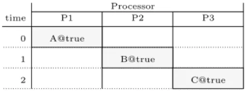
time 0 P2 P1 P3 1 2 A@true B@true C@true Processor
Figure 2: Simple (non-pipelined) scheduling table
• Out(o) ⊆ Cells is the set of cells written by o.
• Guard(o) is the execution condition of o, defined as a predicate over the values of memory cells. We denote with GuardIn(o) the set of memory cells used in the computation of Guard(o).
• Res(o) ⊆ P is the set of processors used during the execution of o. • t(o) is the start date of o.
• d(o) is the duration of o. The duration is viewed here as a time budget the operation must not exceed. This can be statically ensured through a worst-case execution time analysis.
All the resources of Res(o) are exclusively used by o after t(o) and for a duration of d(o) in cycles where Guard(o) is true. The sets In(o) and Out(o) are not necessarily disjoint, to model variables that are both read and updated by an operation. For lifetime analysis purposes, we assume that input and output cells are used for all the duration of the operation. The cells of GuardIn(o) are all read at the beginning of the operation, but we assume the duration of the computation of the guard is negligible (zero time).2
To cover cases where a memory cell is used by one operation before being updated by another, each memory cell can have an initial value. For a memory cell m, Init(m) is either nil, or some constant.
The simple scheduling table pictured in Fig. 2 uses the architecture of Fig. 1. It has a length of 3 and contains 3 operations (A, B, and C). Operation A reads no memory cell, but writes v1, so that In(A) = ∅ and Out(A) = {v1}. Similarly,
In(B) = {v1}, Out(B) = In(C) = {v2}, and Out(C) = ∅. All 3 operations are
executed at every cycle, so their guard is true (guards are graphically represented with “@true”). The 3 operations are each allocated on one processor: Res(A) = {P1}, Res(B) = {P2}, Res(C) = {P3}. Finally, t(A) = 0, t(B) = 1, t(C) = 2,
and d(A) = d(B) = d(C) = 1. No initialization of the memory cells is needed (the initial states are all nil).
2.3
Well-formed properties
The formalism above provides the syntax of our implementation models, and allows the definition of operational semantics. However, not all syntactically
2The memory access model where an operation reads its inputs at start time, writes its outputs upon completion, and where guard computations take time can be represented on top of our model.
P1 P2 P3 A@true iteration 1 0 A@true iteration 2 A@true iteration 3 A@true iteration 4 B@true iteration 1 B@true iteration 2 B@true iteration 3 C@true iteration 1 C@true iteration 2 1 2 3 Prologue Steady state . . . . time
Figure 3: Pipelined execution trace
correct specifications model correct implementations. Some of them are non-deterministic due to data races or due to operations exceeding their time bud-gets. Others are simply un-implementable, for instance because an operation is scheduled on processor P , but accesses memory cells on a RAM block not connected to P . A set of correctness properties is therefore necessary to define the well-formed implementation models.
However, some of these properties are not important in this paper, because we assume that the input of our pipelining technique is already correct. Our pipelining techniques will preserve most correctness properties because they preserve all allocation and scheduling choices inside each execution cycle. We only formalize here two correctness properties that will need attention in the following sections.
We say that two operations o1 and o2 are non-concurrent, denoted o1⊥o2, if
either their executions do not overlap in time (t(o1) + d(o1) ≥ t (o2) or t (o2) +
d(o2) ≥ t (o1)), or if they have exclusive guards (Guard(o1) ∧ Guard(o2) = false).
With this notation, the following correctness properties are assumed respected by input (non-pipelined) implementation models, and must be respected by the output (pipelined) model:
Sequential processors. No two operations can use a processor at the same time. Formally, for all o1, o2∈ O, if Res(o1) ∩ Res(o2) 6= ∅ then o1⊥o2.
No data races. If some memory cell m is written by o1 (m ∈ Out(o1)) and is
used by o2(m ∈ In(o2) ∪ Out(o2)), then o1⊥o2.
3
Pipelining technique overview
In this section, we define our model of pipelined implementation, which builds over the non-pipelined one, enriching it with temporal information. We also ex-plain how a pipelined implementation is constructed once the pipelining analysis (described later in the paper) has been performed.
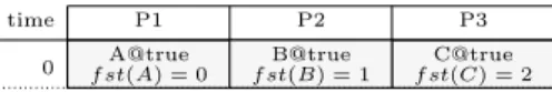
For the example in Fig. 2, an execution where successive cycles do not overlap in time is clearly sub-optimal. Our objective is to allow the pipelined execution of Fig. 3, which ensures a maximal use of the computing resources. In the pipelined execution, a new instance of operation A starts as soon as the previous one has completed, and the same is true for B and C. The first two time units of the execution are the prologue which fills the pipeline. In the steady state the pipeline is full and has a throughput of one computation cycle (of the non-pipelined system) per time unit. If the system is allowed to terminate,
time P1 P2 P3 0 f st(A) = 0A@true f st(B) = 1B@true f st(C) = 2C@true
Figure 4: Pipelined scheduling table
then completion is realized by the epilogue, not pictured in our example, which empties the pipeline.
We represent this pipelined implementation using the pipelined scheduling table pictured in Fig. 4. Its length is 1, corresponding to the throughput of the pipelined system. The operation set contains the same operations A, B, and C, but there are significant changes. The start dates of B and C are now 0, as the 3 operations are started at the same time in each pipelined cycle. To avoid confusion, we reserve the name computation cycle for full computations, as specified by the initial scheduling table. A computation cycle spans over several pipelined cycles, but each pipelined cycle starts exactly one computation cycle. To account for the prologue phase, where operations progressively start to execute, each operation is assigned a start index fst(o). If an operation o has fst(o) = n it will first be executed in the pipelined cycle of index n (indices start at 0). Due to pipelining, the instance of o executed in the pipelined cycle m belongs to the computation cycle of index m − fst(o). For instance, operation C with fst(C) = 2 is first executed in the 3rd repetition of the table (of index
2), but belongs to the first computation cycle.
Note that the prologues of our pipelined implementations are obtained by incremental activation of the steady state operations. This property, which allows periodic implementation, is not present in classical software pipelining approaches. Periodicity, plus the requirement that the pipelined implementa-tion executes each computaimplementa-tion cycle as specified by the non-pipelined table, means that the pipelined scheduling table can be fully built using Procedure 1 starting from the non-pipelined table and from the period of the pipelined sys-tem. The procedure first determines the start index and new start date of each operation by folding the non-pipelined table onto the new period. Procedure AssembleSchedule then determines which memory cells need to be replicated due to pipelining, using the technique provided in Section 3.2.
Algorithm 1 BuildSchedule
Input: S : non-pipelined scheduling table b
p : new period of the system Output: bS : pipelined schedule table
for all o in O do fst(o) := [t(o)pb ] b
t(o) := t (o) − fst(o) ∗ bp b
S := AssembleSchedule(S, bp, fst, bt)
When comparing with existing software pipelining techniques, the most ob-vious difference is that our approach allows optimization along a single degree of freedom (the period). Resource allocation and scheduling inside a computation cycle are fixed. This approach limits the throughput optimization space.
How-ever, throughput optimization is not our only objective. As explained in the introduction, we apply our transformations as part of a larger implementation flow. In this flow, the pipelining phase must preserve the end-to-end latency guarantees of each computation cycle (ensured by other tools), and the periodic implementation model. Our approach satisfies these requirements. A simpler pipelining technique also has the advantage of speed, and of allowing us to fo-cus on the predication-related issues, where the real complexity and gain of our approach stands. The approach also gives good results on real-life scheduling problems.
3.1
Dependency graph and maximal throughput
In our approach, the period of the pipelined system is determined by the data dependencies between successive execution cycles. We represent these depen-dencies as a Data Dependency Graph (DDG) – a formalism that is classical in software pipelining based on modulo scheduling techniques[3]. In this section we define DDGs and we explain how the new period is computed from them. The computation of DDGs is detailed in Section 4.
Given an implementation model S =< p, O, Init >, the DDG associated to S is a directed graph DG =< O, V > where V ⊆ O × O × N. Ideally, the elements of V are all the triples (o1, o2, n) such that there exists an execution of the
implementation and a computation cycle k such that operation o1 is executed
in cycle k, operation o2is executed in cycle k+n, and o1must be executed before
o2, for instance because some value produced by o1 is used by o2. In practice,
any V including all the arcs defined above (any over-approximation) will be acceptable, leading to correct (but possibly sub-optimal) implementations.
The DDG represents all possible dependencies between operations, both inside a cycle (when n = 0) and between successive cycles at distance n ≥ 1. Given the statically scheduled implementation model, with fixed dates for each operation, the pipelined schedule must respect unconditionally all these dependencies.
For each operation o ∈ O, we denote with tn(o) the date where operation
o is executed in cycle n, if its guard is true. By construction, we have tn(o) =
t(o) + n ∗ p. In the pipelined implementation of period bp, this date is changed to btn(o) = t (o) + n ∗ bp. Then, for all (o1, o2, n) ∈ V and k ≥ 0, the pipelined
implementation must satisfy btk+n(o2) ≥ btk(o1) + d(o1), which implies:
b
p ≥ max(o1,o2,n)∈V,n6=0⌈
t(o1)+d(o1)−t(o2)
n ⌉
Our objective is to build pipelined schedules satisfying this lower bound con-straint and which are well-formed in the sense of Section 2.3.
3.2
Memory management issues
Assuming that bS is the pipelined version of S, we denote with max_par = ⌈len(S)/len( bS)⌉ the maximal number of simultaneously-active computation cy-cles of the pipelined implementation. Note that max_par = 1 + maxo∈Ofst(o).
Consider now our example. In its non-pipelined version, both A and B use memory cell v1at each cycle. In the pipelined table A and B work in parallel, so
is rep(v1) = 2. Each memory cell v is assigned its own replication factor, which
must allow concurrent computation cycles using different copies of v to work without interference. Obviously, we can bound rep(v) by max_par. We use a tighter margin, based on the observation that most variables (memory cells) have a limited lifetime inside a computation cycle. We set rep(v) = 1 + lst(v) − fst(v), where:
fst(v) = minv∈In(o)∪Out(o)fst(o) lst(v) = maxv∈In(o)∪Out(o)fst(o)
Through replication, each memory cell v of the non-pipelined scheduling table is replaced by rep(v) memory cells, allocated on the same memory block as v, and organized in an array v, whose elements are v[0], . . . , v[rep(v) − 1]. These new memory cells are allocated cyclically, in a static fashion, to the successive computation cycles. More precisely, the computation cycle of index n is assigned the replicas v[n mod rep(v)] for all v. The computation of rep(v) ensures that if n1and n2 are equal modulo rep(v), but n16= n2, then computation cycles n1
and n2 cannot access v at the same time.
For systems like our simple example, where no information is passed from one computation cycle to the next, this static allocation allows for a simple code generation, which consists in replacing v with v[(cid − fst(o)) mod rep(v)] in the input and output parameter lists of every operation o that uses v. Here, cid is the index of the current pipelined cycle. It is represented in the generated code by an integer. When execution starts, cid is initialized with 0. At the start of each subsequent pipelined cycle, it is updated to (cid + 1) mod R, where R is the least common multiple of all the values rep(v).
When a computation cycle uses values produced by previously-started com-putation cycles,3 code generation is more complicated, because a computation
cycle may access memory cells different than its own. The code generation problem is complicated by the fact that it is impossible, in the general case, to statically determine which cell must be read (because the cell was written at an arbitrary distance in time). Thus, we need a dynamic mechanism to identify which cell to read. If more static pipelined implementations are needed, different pipelining techniques should be designed, either limiting the class of accepted non-pipelined systems, or allowing the copying of one memory cell onto another, which we do not allow because it may introduce timing penalties.
Our memory access mechanism is supported by a new data structure which associates to each memory cell v of the non-pipelined scheduling table an array src(v) of length rep(v), and allocated on the same memory block as v. In this context, code is generated as follows:
At execution start, all the values of src are initialized with 0 (pointing to the initial values of the memory cells).
At the start of each pipelined cycle, for each cell v of the initial scheduling table, assign to
src(v)[(cid − fst(v)) mod rep(v)] the value of
src(v)[(cid − fst(v) − 1) mod rep(v)]. This assignment indicates that the value of v initially used during computation cycle cid is that used (but not neces-sarily produced) during computation cycle cid − 1 and stored in memory cell v[src(v)[(cid − fst(v) − 1) mod rep(v)]].
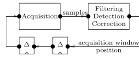
∆ ∆ Acquisition Correction Detection Filtering samples acquisition window position
Figure 5: Knock control functional specification
When an operation o of the non-pipelined scheduling table reads v, its coun-terpart in the pipelined table will read v[src(v)[(cid − fst(o)) mod rep(v)]]. The same is true for cells used by the computation of execution conditions.
When o writes v in the non-pipelined table, there are 2 cases: If o also reads v, then the counterpart of o in the pipelined table will write the same memory cell it reads (as defined above). If o does not read v, then o writes the memory cell normally assigned to this computation cycle by the replication process (v[x], where
x = (cid − fst(o)) mod rep(v)). An operation is added after o and on the same execution condition to set src(v)[x] to x.
The last aspect of memory management is initialization. In our case, v1
requires no initialization, so that none of its replicas do. In the general case, if Init(v) 6= nil, we need to initialize v[0] with Init(v), but not the other replicas.
3.3
The knock control example
We complete this section with a larger example that illustrates several key points of our approach, including the use of conditional scheduling tables and the pipelining of sporadic systems. Knock control is one of the functions of the engine control unit (ECU) of gasoline spark-ignition engines. At each rota-tion of the engine, it chooses for each cylinder an ignirota-tion time that maximizes power output while keeping engine-destructive knocks (autoignition events) at an acceptable level.
We provide in Fig. 5 a simplified high-level description of the knock control functionality. The model is based on an industrial case study and on the de-scription of [4]. The behavior is as follows: One computation cycle is triggered at each rotation of the engine crankshaft. The cycle starts with the acquisition of knock noise data. Acquisition is performed over a knock acquisition window where autoignition can occur. It is performed using a vibration sensor sampled at 100kHz, and the samples are stored in a buffer. The samples are used by the filtering, detection, and correction (FDC) function to adjust the ignition time (not figured here) and the position and size of the acquisition window. The configuration data produced by the computation cycle of index n controls the acquisition of cycle n + 2. This delayed feedback is realized using two unit delays (labeled ∆). Acquisition is performed by a specialized device (labeled AD in Fig. 6) of the ECU, whereas the FDC function is computed by the ECU microcontroller (µC).
For reasons related to the physics of engines and to computing resource limitations in the ECU, the successive computation cycles must sometimes be pipelined, by allowing the acquisition and FDC operations of successive cycles to be executed in parallel. Such a pipelining can be directly constructed using
buf2 config0 config1 config2 c device µC RAM BUF2_mem Acquisition (AD) BUF2 BUF1_mem buf1 BUF1
Figure 6: Engine control unit (ECU) architecture
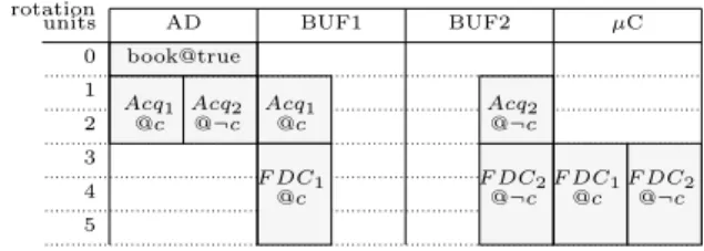
Acq1 @c Acq2 @¬c @c @c F DC1 book@true @¬c F DC2 F DC1 @c F DC2 @¬c Acq2 @¬c Acq1 3 2 1 0 4 5 µC BUF2 BUF1 rotation units AD
Figure 7: Non-pipelined scheduling table for the knock control
our approach, using the code generation scheme of the previous section. How-ever, our code generation may conflict with memory constraints or pre-existent implementation choices. We will assume here that the system designers have already fixed the maximal number of buffers to 2, placed them at fixed places in memory, and written the protocol that alternates the use of the buffers in both acquisition and FDC. The remaining difficulties are the computation of the pipelined period and the management of all memory cells that are not con-strained.
Representing the memory replication constraints is best done as in Fig. 6, with two memory cells (buf 1 and buf 2) on separate memory blocks (BUF1_mem, resp. BUF2_mem). Each memory block has its own memory controller (BUF1, resp. BUF2) that ensures exclusive access and makes memory cell replication impossible during pipelining.
In this implementation model, the scheduling table of one computation cycle is represented in Fig. 7. Memory cell c is a Boolean used in guards to determine which buffer to use in the current computation cycle to pass data from the acquisition function to F DC. In the beginning of each computation cycle, the bookkeeping operation book flips the value of c by executing “c:=¬c”. In cycles where the new value is true, buffer buf 1 is used. Otherwise, buf 2 is used. If we denote with cnthe value of c used in guards throughout computation cycle n, we
have cn= ¬cn−1for all n positive. The bookkeeping operation also implements
the function of the unit delays.
The scheduling table represents both activation scenarios, corresponding to different initial values of c. In order not to introduce special memory access operations, we split the acquisition and F DC operations in two. Both Acq1
and Acq2 perform acquisition. But the first writes its samples in buf 1 and is
3 2 1 0 4 5 Acq12 Acq 2 2 book2 @true 8 7 6 . . . . . . . Acq10 Acq 0 2 F DC01 book0 @true book1@true Acq1 1 F DC11 Acq1 2 Acq10 Acq1 1 Acq02 Acq1 2 F DC20F DC 0 1F DC 0 2 @c0 @¬c0 @c0 @c0 @c1 @c1 @¬c1 @¬c1 @¬c0 @c0 @¬c0 @¬c0 @c1 @c2 @¬c2 @c2 Acq12 F DC21 Acq22 F DC12F DC 1 1 @¬c1 @c1 @¬c2 @¬c1 BUF1 BUF2 µC units rotation AD
Figure 8: Pipelined execution of the knock control
AD BUF1 BUF2 µC 2 1 0 book@true Acq2 @¬cn
Acq1 Acq1 Acq2
@cn @¬cn @cn f st = 1 f st = 1f st = 1f st = 1 F DC1 F DC2F DC1F DC2 @ @ @ @ cn−1 ¬cn−1 cn−1¬cn−1 units rotation
Figure 9: Pipelined scheduling table for the knock control
by ¬c. Each of the Acqi and F DCi operations use two resources: One of AD
and µC and one of the memory controllers BUF1 and BUF2.
The operation durations must be interpreted here as upper WCET bounds in an engine rotation referential. More precisely, each duration gives the max-imal rotation (in degrees) of the engine crankshaft during the execution of the operation. For the acquisition operation, this is the maximal acquisition window size. The FDC function runs on a microcontroller, and its duration is charac-terized with a classical WCET (in real time). Conversion to the engine rotation referential is performed by assuming the maximal engine rotation speed.
The algorithms of the next section determine that successive computation cycles can be at best pipelined as pictured in Fig. 8. To do so, they determine that cn= ¬cn−1for all n, thus allowing the acquisition and F DC operations of
successive computation cycles to be executed in parallel. Note that a resource can be allocated to two operations at the same date if their guards are exclusive. Like in Fig. 7, we represent here both activation scenarios, corresponding to different initial values of c.
The corresponding pipelined scheduling table is provided in Fig. 9. The sys-tem is schedulable if the length of this table is smaller than the engine rotation interval between successive triggers of computation cycles. In turn, this is given by the number of cylinders and structure of the engine. If the system is schedu-lable, the code generation technique of Section 3.2 can be used to automatically generate the book keeping memory cells and code. Thus, we automate the analysis of [4] and also allow automatic code generation.
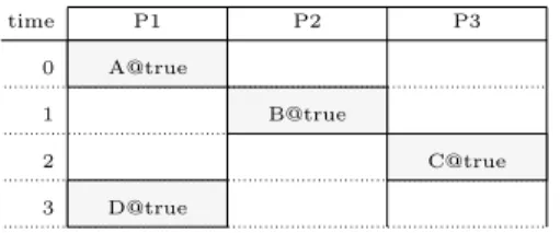
time 0 P2 P1 P3 1 2 A@true B@true C@true D@true 3
Figure 10: Dependency analysis example, non-pipelined
time P1 P2 P3
0 f st(A) = 0A@true C@true
B@true f st(D) = 1 D@true f st(B) = 0 f st(C) = 1 1
Figure 11: Dependency analysis example, pipelined
4
Dependency analysis and main routine
In this section, we provide algorithms that determine if and when a new com-putation cycle can be started while another one is still active. The core of this computation is a dependency analysis which builds the DDG of Section 3.1. Dependency analysis is performed by the lines 1-10 of Algorithm 3, which act as a driver for Algorithm 2. The remainder of Algorithm 3 uses DDG-derived information to drive the pipelining routine (Algorithm 1).
Both the data dependency analysis and pipelining driver take as input a flag that chooses between two pipelining modes with different complexities and capabilities. To understand the difference, consider the non-pipelined scheduling table of Fig. 10. Resource P1 has an idle period between operations A and B
where a new instance of A can be started. However, to preserve a periodic execution model, A should not be restarted just after its first instance (at date 1). Indeed, this would imply a pipelined throughput of 1, but the fourth instance of A cannot be started at date 3 (only at date 6). The correct pipelining starts A at date 2, and results in the pipelined scheduling table of Fig. 11. Note that the pipelined system is strictly periodic, of period 2, because every instance of D is bound to its slot of size 1 between two instances of A (and vice-versa).
Determining if the reuse of idle spaces between operations is possible requires a complex analysis which looks for the smallest integer n greater than the lower bound of Section 3.1, smaller than the length of the initial table, an such that a well-formed pipelined table of length n can be constructed. This computation is performed by lines 14-17 of Algorithm 3. We do not provide here the code of function WellFormed, which checks the respect of the well-formed properties of Section 2.3.
This complex computation can be avoided when idle spaces between two operations are excluded from use at pipelining time. This can be done by creating a dependency between any two operations of successive cycles that use a same resource and have non-exclusive execution conditions. In this case, the pipelined system period is exactly the lower bound of Section 3.1, and the output scheduling table is produced with a single call to Algorithm 1 (BuildSchedule)
in line 12 of Algorithm 3. Of course, Algorithm 2 needs to consider (in lines 9-12) the extra dependencies.
Excluding the idle spaces from pipelining also has the advantage of support-ing a sporadic execution model. In sporadic systems the successive computation cycles can be executed with the maximal throughput specified by the pipelined table, but can also be triggered arbitrarily less often, for instance to tolerate tim-ing variations, or to minimize power consumption in systems where the demand for computing power varies.
Algorithm 2 DependencyAnalysisStep Inputs: S : non-pipelined scheduling table
l : the list of events of S n : integer (cycle index) fast_pipelining_flag : boolean InputOutputs: S : annotated scheduling table
curr : current variable assignments DDG : Data Dependency Graph
1: S := Concat(S, Annotate(S, n))
2: while l not empty do
3: e := head(l) ; l := tail(l)
4: if e = start(o) then
5: Replace Guard(on) by:
_
wi@Ci∈curr(vi),i=1,k
(C1∧ . . . ∧ Ck) ∧ go(w1, . . . , wk)
where Guard(o) = go(v1, . . . , vk).
6: for all p operation in S, u ∈ Out(p), v ∈ In(o) do
7: if u0p@C ∈ curr(v) and C ∧ Guard(on) 6= false then
8: DDG := DDG∪ {(p0, on, n)}
9: if fast_pipelining_flag then
10: if Res(o) ∩ Res(p) 6= ∅ then
11: if Guard(on) ∧ Guard(p0) 6= false then
12: DDG := DDG∪ {(p0, on, n)}
13: else
14: /* e = end(o) */
15: for all v ∈ Out(o) do
16: new_curr :={vn o@Guard(on)} 17: for all vk p@C ∈ curr(v) do 18: C′ := C ∧ ¬Guard(on) 19: if C′6= false then 20: new_curr := new_curr∪ {vk p@C′} 21: curr(v) := new_curr
The remainder of this section details the dependency analysis phase. The output of this analysis is the lower bound defined in Section 3.1, computed as period_minorant. The analysis is organized around the repeat loop which incrementally computes, for cycle ≥ 1, the DDG dependencies of the type (o1, o2, cycle). The computation of the DDG is not complete: We bound it using
algo-rithm. This condition is based on the observation that if period_minorant ∗ k ≥ len(S) then execution cycles n and n + k cannot overlap in time (for all n).
The DDG computation works by incrementally unrolling the non-pipelined scheduling table. At each unrolling step, the result is put in the SSA-like data structure S that allows the computation of (an over-approximation of) the de-pendency set. Unrolling is done by annotating each instance of an operation o with the cycle n in which it has been instantiated. The notation is on. Putting
in SSA-like form is based on splitting each memory cell v into one version per operation instance producing it (vn
o, if v ∈ Out(o)), and one version for the
ini-tial value (vinit). Annotation and variable splitting is done on a per-cycle basis by the Annotate routine (not provided here) which changes for each operation o its name to on, and replaces Out(o) with {vn
o | v ∈ Out(o)} (n is here the cycle
index parameter). Instances of S produced by Annotate are then assembled into S by the Concat function which simply adds to the date of every operation in the second argument the length of its first argument.
Recall that we are only interested in dependencies between operations in dif-ferent cycles. Then, in each call to Algorithm 2 we determine the dependencies between operations of cycle 0 and operations of cycle n, where n is the current cycle. To determine them, we rely on a symbolic execution of the newly-added part of S, i.e. the operations ok with k = n. Symbolic execution is done through
a traversal of list l, which contains all operation start and end events of S, and therefore S, ordered by increasing date. For each operation o of S, l contains two elements labeled start(o) and end(o). The list is ordered by increasing event date using the convention that the date of start(o) is t(o), and the date of end(o) is t(o) + d(o). Moreover, if start(o) and end(o′) have the same date,
the start(o) event comes first in the list.
At each point of the symbolic execution, the data structure curr identifies the possible producers of each memory cell. For each cell v of the initial table, curr(v) is a set of pairs w@C, where w is a version of v of the form vk
o or vinit,
and C is a predicate over memory cell versions. In the pair w@C, C gives the condition on which the value of v is the one corresponding to its version w at the condidered point in the symbolic simulation. Intuitively, if vk
o@C ∈ curr(v), and
we symbolically execute cycle n, then C gives the condition under which in any real execution of the system v holds the value produced by o, n−k cycles before. The predicates of the elements in curr(v) provide a partition of true. Initially, curr(v) is set to {vinit@true} for all v. This is changed by Algorithm 2 (lines 15-21), and by the call to InitCurr in Algorithm 3. We do not provide this last function, which performs the symbolic execution of the nodes of S annotated with 0. Its code is virtually identical to that of Algorithm 2, lines 1 and 6-12 being excluded.
At each operation start step of the symbolic execution, curr allows us to complete the SSA transformation by recomputing the guard of the current op-eration over the split variables (line 5 of Algorithm 2). In turn, this allows the computation of the dependencies (lines 6-12). Predicate comparisons are han-dled by a SAT solver that also considers a Boolean abstraction of the operations of the algorithm. In our knock control example, the Boolean abstraction of the book operation provides the information that cn= ¬cn−1.
Algorithm 3 PipeliningDriver
Input: S : non-pipelined schedule table fast_pipelining_flag : boolean Output: bS : pipelined schedule table
1: l := BuildEventList(S) 2: period_minorant := 0 3: cycle := 0 4: S := Annotate(S, cycle) 5: curr := InitCurr(S) 6: repeat 7: cycle:=cycle + 1 8: (S, curr, DDG) := DependencyAnalysisStep(S, l, cycle,fast_pipelining_flag, S, curr, DDG) 9: period_minorant := max(period_minorant, max(o1,o2,cycle)∈DDG⌈ t(o1)+d(o1)−t(o2) cycle ⌉ )
10: until period_minorant∗ cycle ≥ len(S)
11: if fast_pipelining_flag then
12: bS := BuildSchedule(S, period_minorant)
13: else
14: for new_period := period_minorant to len(S) do
15: S := BuildSchedule(S, new_period)b
16: if WellFormed(bS) then
17: goto 18
18: return
5
Experimental results
We have applied our pipelining algorithms on 3 significant, real-life examples of real-time implementation problems (there are no standardized benchmarks). The results are synthesized in Table 12.
The largest example we use is the embedded control application of the CyCab electric car [15]. The control application we use allows the CyCab to be driven manually or in an autonomous “platooning” mode where it follows the vehicle in front of it, letting it make the speed and direction change decisions. The embedded software runs on a platform composed of 3 micro processors connected through a CAN bus. Our pipelining technique allows a significant reduction of 27% in cycle time. This reduction means that the application can be significantly complexified while maintaining I/O latency.
Scheduling table length example initial pipelined gain
cycab 1482 1083 27%
ega 84 79 6%
knock 6 3 50%
simple 3 1 66%
The second example is an adaptive equalizer. This filter is normally part of a larger control application, but we considered it here in isolation. The particularity of this example is that it has already been carefully designed to exploit the parallelism of the execution platform (it can be seen as “manually pipelined”). The cycle length reduction after application of our technique is not very large, but it is still significant in spite of the very optimized starting point. The third example is the knock controller of Section 3.3. We also add a line for our toy example. The comparison is interesting, because this example allows for an ideal pipelining with a resource usage of 100%.
6
Conclusion
We have defined a latency-preserving software pipelining approach allowing the optimization of the throughput of periodic and sporadic real time systems de-fined through predicated scheduling tables. We apply it on the output of well-established latency-optimizing scheduling tools, resulting in a scheduling flow that optimizes latency and throughput, with priority to latency. We applied our technique, with good results, on several real-life systems.
Many open problems remain. One of them is the exploitation of execution guards over partitioned architectures. Using the n-synchronous formalism[7] should allow us to express and exploit regular repetition patterns in the pipelin-ing process. Another important goal is to integrate pipelinpipelin-ing in the initial scheduling process, so that different trade-offs between latency, throughput, and resource usage can be obtained.
Acknowledgement. The authors wish to thank Albert Cohen for having in-troduced them to the field of software pipelining.
References
[1] ARINC 653: Avionics application software standard interface. www.arinc.org, 2005. [2] Autosar (automotive open system architecture), release 4. http://www.autosar.org/,
2009.
[3] V. H. Allan, R. B. Jones, R. M. Lee, and S. J. Allan. Software pipelining. ACM Com-puting Surveys, 27(3), 1995.
[4] C. André, F. Mallet, and M.-A. Peraldi-Frati. A multiform time approach to real-time system modeling; application to an automotive system. In Proceedings SIES, Lisbon, Portugal, July 2007.
[5] P. Caspi, A. Curic, A. Magnan, C. Sofronis, S. Tripakis, and P. Niebert. From Simulink to SCADE/Lustre to TTA: a layered approach for distributed embedded applications. In Proceedings LCTES, San Diego, CA, USA, June 2003.
[6] Yi-Sheng Chiu, Chi-Sheng Shih, and Shih-Hao Hung. Pipeline schedule synthesis for real-time streaming tasks with inter/intra-instance precedence constraints. In DATE, Grenoble, France, 2011.
[7] A. Cohen, M. Duranton, C. Eisenbeis, C. Pagetti, F. Plateau, and M. Pouzet. N-synchronous kahn networks: a relaxed model of synchrony for real-time systems. In Proceedings POPL’06. ACM Press, 2006.
[8] P. Eles, A. Doboli, P. Pop, and Z. Peng. Scheduling with bus access optimization for distributed embedded systems. IEEE Transactions on VLSI Systems, 8(5), Oct 2000. [9] G. Fohler, A. Neundorf, K.-E. Årzén, C. Lucarz, M. Mattavelli, V. Noel, C. von
Platen, G. Butazzo, E. Bini, and C. Scordino. EU FP7 ACTORS project. Deliver-able D7a: State of the art assessment. Ch. 5: Resource reservation in real-time systems. http://www3.control.lth.se/user/karlerik/Actors/d7a-rev.pdf, 2008.
[10] T. Grandpierre and Y. Sorel. From algorithm and architecture specification to automatic generation of distributed real-time executives. In Proceedings MEMOCODE, Mont St Michel, France, 2003.
[11] J.L. Hennessy and D.A. Patterson. Computer Architecture: A Quantitative Approach. Morgan Kaufmann, 4thedition, 2007.
[12] A. Monot, N. Navet, F. Simonot, and B. Bavoux. Multicore scheduling in automotive ECUs. In Proceedings ERTSS, Toulouse, France, 2010.
[13] L. Morel. Exploitation des structures régulières et des spécifications locales pour le de-veloppement correct de systèmes réactifs de grande taille. PhD thesis, Institut National Polytechnique de Grenoble, 2005.
[14] D. Potop-Butucaru, A. Azim, and S. Fischmeister. Semantics-preserving implementa-tion of synchronous specificaimplementa-tions over dynamic TDMA distributed architectures. In Proceedings EMSOFT, Scottsdale, Arizona, USA, 2010.
[15] C. Pradalier, J. Hermosillo, C. Koike, C. Braillon, P. Bessière, and C. Laugier. The CyCab: a car-like robot navigating autonomously and safely among pedestrians. Robotics and Autonomous Systems, 50(1), 2005.
[16] B.R. Rau and C.D. Glaeser. Some scheduling techniques and an easily schedulable hori-zontal architecture for high performance scientific computing. In Proceedings of the 14th annual workshop on Microprogramming, IEEE, 1981.
[17] J. Rushby. Bus architectures for safety-critical embedded systems. In Proceedings EM-SOFT’01, volume 2211 of LNCS, Tahoe City, CA, USA, 2001.
[18] M. Smelyanskyi, S. Mahlke, E. Davidson, and H.-H. Lee. Predicate-aware scheduling: A technique for reducing resource constraints. In Proceedings CGO, San Francisco, CA, USA, March 2003.
[19] N.J. Warter, D. M. Lavery, and W.W. Hwu. The benefit of predicated execution for software pipelining. In HICSS-26 Conference Proceedings, Houston, Texas, USA, 1993. [20] H.-S. Yun, J. Kim, and S.-M. Moon. Time optimal software pipelining of loops with
control flows. International Journal of Parallel Programming, 31(5):339–391, October 2003.
[21] W. Zheng, J. Chong, C. Pinello, S. Kanajan, and A. Sangiovanni-Vincentelli. Extensible and scalable time-triggered scheduling. In Proceedings ACSD, St. Malo, France, June 2005.
Centre de recherche INRIA Bordeaux – Sud Ouest : Domaine Universitaire - 351, cours de la Libération - 33405 Talence Cedex Centre de recherche INRIA Grenoble – Rhône-Alpes : 655, avenue de l’Europe - 38334 Montbonnot Saint-Ismier Centre de recherche INRIA Lille – Nord Europe : Parc Scientifique de la Haute Borne - 40, avenue Halley - 59650 Villeneuve d’Ascq
Centre de recherche INRIA Nancy – Grand Est : LORIA, Technopôle de Nancy-Brabois - Campus scientifique 615, rue du Jardin Botanique - BP 101 - 54602 Villers-lès-Nancy Cedex
Centre de recherche INRIA Rennes – Bretagne Atlantique : IRISA, Campus universitaire de Beaulieu - 35042 Rennes Cedex Centre de recherche INRIA Saclay – Île-de-France : Parc Orsay Université - ZAC des Vignes : 4, rue Jacques Monod - 91893 Orsay Cedex
Centre de recherche INRIA Sophia Antipolis – Méditerranée : 2004, route des Lucioles - BP 93 - 06902 Sophia Antipolis Cedex
Éditeur
INRIA - Domaine de Voluceau - Rocquencourt, BP 105 - 78153 Le Chesnay Cedex (France)