Experimenting with the p4est library for AMR simulations of two-phase flows

HAL Id: hal-01591956

https://hal.archives-ouvertes.fr/hal-01591956

Submitted on 22 Sep 2017

HAL is a multi-disciplinary open access

archive for the deposit and dissemination of

sci-entific research documents, whether they are

pub-lished or not. The documents may come from

teaching and research institutions in France or

abroad, or from public or private research centers.

L’archive ouverte pluridisciplinaire HAL, est

destinée au dépôt et à la diffusion de documents

scientifiques de niveau recherche, publiés ou non,

émanant des établissements d’enseignement et de

recherche français ou étrangers, des laboratoires

publics ou privés.

Experimenting with the p4est library for AMR

simulations of two-phase flows

Florence Drui, Alexandru Fikl, Pierre Kestener, Samuel Kokh, Adam Larat,

Vincent Le Chenadec, Marc Massot

To cite this version:

Florence Drui, Alexandru Fikl, Pierre Kestener, Samuel Kokh, Adam Larat, et al.. Experimenting

with the p4est library for AMR simulations of two-phase flows. ESAIM: Proceedings and Surveys,

EDP Sciences, 2016, 53, pp.232 - 247. �10.1051/proc/201653014�. �hal-01591956�

ESAIM: PROCEEDINGS AND SURVEYS,Vol. ?, 2017, 1-10 Editors: Will be set by the publisher

EXPERIMENTING WITH THE P4EST LIBRARY FOR AMR SIMULATIONS

OF TWO-PHASE FLOWS.

Florence Drui

, Alexandru Fikl

, Pierre Kestener

, Samuel Kokh

,

Adam Larat

, Vincent Le Chenadec

and Marc Massot

Abstract. Many physical problems involve spatial and temporal inhomogeneities that require a very fine discretization in order to be accurately simulated. Using an adaptive mesh, a high level of resolution is used in the appropriate areas while keeping a coarse mesh elsewhere. This idea allows to save time and computations, but represents a challenge for distributed-memory environments. The MARS project (for Multiphase Adaptative Refinement Solver) intends to assess the parallel library p4est for adaptive mesh, in a case of a finite volume scheme applied to two-phase flows. Besides testing the library’s performances, particularly for load balancing, its user-friendliness in use and implementation are also exhibited here. First promising 3D simulations are even presented.

Résumé. De nombreux problèmes physiques mettent en jeu des inhomogénéités spatiales et tem-porelles, qui pour être simulées correctement requièrent une discrétisation très fine. Utiliser un maillage adaptatif pour obtenir ce niveau de résolution dans les zones où elle est requise, et garder un maillage grossier en-dehors, permet d’intéressantes économies en temps et ressources de calcul, mais représente un défi pour le calcul distribué. Le projet MARS (Multiphase Adaptative Refine-ment Solver ) a pour objectif d’évaluer la librairie parallèle de maillage adaptatif p4est, appliquée à un schéma de volumes finis pour un modèle bifluide d’écoulement diphasique. Outre les perfor-mances de cette librairie, en particulier en terme d’équilibrage de charge, sa facilité d’utilisation et d’implémentation sont mises en avant. Des premières simulations 3D prometteuses sont présentées.

1. Introduction

Adaptive Mesh Refinement (AMR) methods have been developed to solve problems dealing with phe-nomena appearing at multiple and very different spatial and temporal scales. It is especially useful in the resolution of the dynamics of localized fronts or interfaces in plasma physics, reactive and complex flows [18]. Combustion problems usually involve a very thin and localized flame front coupled to the hydrodynamics of the flow [19]. In this project, we are more specifically looking at problems of diffuse interface modeling for two-phase flows, where a good precision is needed for describing the dynamics of the interface between the two phases.

One of the first comprehensive descriptions of AMR was given in [4], with an application to hyperbolic partial differential equations. This paper was followed by an extension of the method which accounts for the presence of shocks and greatly simplified the AMR-related algorithms [3]. Since then, AMR concepts have been implemented in dedicated application codes such as RAMSES [34] in astrophysics, or Gerris [31] for fluid and two-phase flow studies, among others. They mostly follow the ideas of the Fully Threaded Tree of

1_{Laboratoire EM2C, CNRS UPR 288 et École Centrale Paris, Grande Voie des Vignes, 92295 Châtenay-Malabry Cédex} 2_{Maison de la Simulation, CNRS USR 1441, Bat. 565 - Digitéo, CEA Saclay, 91191 Gif-sur-Yvette}

3_{CEA/DEN/DANS/DM2S/STMF, CEA Saclay, 91191 Gif-sur-Yvette}

4_{Fédération de Mathématiques de l’École Centrale Paris, CNRS FR 3487, Grande Voie des Vignes, 92295 Châtenay-Malabry}

Cédex

c

(a) Example of overlapped grids illustrating block-based AMR. (b) Example of cell refinement process illustrating cell-based AMR.

Figure 1. Illustration of two approaches to locally refined meshes.

Khokhlov [25]. These tree-based AMR techniques are close, in terms of implementation to the fully adaptive multiresolution scheme (MR) introduced in [14, 29] from the ideas of Harten [22] and used in the MBARETE, z-code codes [17, 19] for various applications.

Unfortunately, these dedicated AMR or MR codes often lead to complex software designs due to the meth-ods employed and suffer heavy difficulties in the development of new applications since the numerical method and the AMR technique are closely entangled. In particular, the problem of domain decomposition and load balancing for parallel computing in both shared and distributed memory architectures is very delicate and necessitates costly complex methods coming from graphs partitioning theory [8, 17]. Recently, several excep-tions offering generic "hands-off " AMR frameworks have appeared such as CHOMBO [1] or p4est [9]. These can be used with any solver or numerical scheme and do not necessarily rely on the Fully Threaded Tree ideas.

Many other AMR codes exist and we suggest the interested reader to look at the survey article [21] for a large review of several such frameworks.

In the context of the MARS project, we have created an interface between a two-phase flow finite volume solver and a dedicated cell-based AMR library: p4est [9]. The objectives are to test the user-friendliness and the performances of the library in the context of HPC and to reveal its advantages and disadvantages compared with simple, non-adaptive algorithms.

The first part of this proceeding describes the principles of AMR methods and, more specifically, the way p4est works. In the second part, we present the two-fluid homogeneous equilibrium model, derived from [12], that involves a system of three conservative equations (in 1D) for an isothermal system of two fluids. The discretization of these PDEs is performed through finite volume techniques and a Godunov-like scheme: the Riemann problems at cells interfaces are solved approximately thanks to Suliciu’s relaxation method (see [7, 33]). Second order approximations using a MUSCL-Hancock scheme (see [37]) were also tested.

Several test cases are performed in order to evaluate different aspects of p4est library and of the numerical methods. They are presented in the last part of this paper, with dedicated implementation details. The two-phase model is finally tested in some realistic 2D and 3D configurations.

2. p4est Library: Description and Specificities

2.1. Presentation of AMR Techniques

There are multiple approaches for adapting a mesh to a specific problem, among which block-based AMR (see Figure 1a), cell-based AMR (Figure 1b) or Wavelet-based AMR, also called adaptive Multi-Resolution (MR) [14, 29, 32], which can lead to error control on the solution. Mesh-free methods, such as the Smoothed Particle Hydrodynamics method and their multi-scale version [2, 13, 16, 26, 28], have also been successfully

employed to offer an adapted discretization. Here, we are only interested in mesh-based methods, and more particularly in cell-based AMR. The cell-based method involves modifications on an initial coarse mesh (usually a single cell representing a rectangular domain) by means of recursively dividing its elements into multiple sub-elements with a fixed ratio. Because of the continuously changing mesh, it is a large departure from the usual methods involving static discretizations. To deal with the constant modifications, cell-based AMR employs trees to store the mesh and easily refine and coarsen specific cells. Different types of trees are used to store the individual refinements of each cell: binary trees for 1D domains, quadtrees for 2D domains, and octrees for 3D (see Figure 2).

2.2. Challenges in cell-based AMR

Unlike block-based AMR, where trees are only used to handle the grid hierarchy, cell-based AMR makes heavy use of tree structures to store the mesh and modify it. The use of this new data structure implies new difficulties in implementing numerical methods (new integration routines, storage strategies and load balancing techniques need to be developed). Indeed, during a simulation, different pieces of information about the tree structure needs to be accessible permanently. Such a requirement raises several issues, especially in high performance environments:

‚ Tree storage, that can be made in linear arrays, but then raises issues of cache locality; ‚ Tree partitioning for a better load balancing between computing processors;

‚ Scalable algorithms;

‚ Representation of complex geometries and not only square or rectangular domains.

Another challenge is to include these tools into existing codes that need to preserve their original data structures.

Over time, various implementation choices have been made to deal with these issues. Recently, linear tree storage, in the form of hash-maps or linear arrays, has been preferred to pointer-based tree representation [17, 18, 24]. These solutions have proved to use less memory than, for example, Fully Threaded Trees [25], have a better cache locality and are easier to parallelize.

p4est is one recent example of a cell-based AMR implementation that uses linear storage given by a space-filling curve. The primary usage of space filling curves in numerical simulation, is to provide a simple and efficient way of partitioning data for load balancing in distributed computing, but they can also be used for organizing data memory layout as in p4est. Indeed, many space filling curves have a nice property called compactness, which can be stated as: contiguity along the space-filing curve index implies, to a certain extend, contiguity in the N-dimensional space of the Cartesian mesh. As a consequence of the compactness property, one can expect also improved AMR performance due to a better cache memory usage resulting from a certain degree of preserved locality between the computational mesh and the data memory layout. p4est also implements specialized refining, coarsening and iterating algorithms for its specific choice of linear storage that have proven scalability [9]. These points are real advantages in the frame of HPC where time and space complexity have to be handled with extreme care. On the top of that, the concept of forest of trees, allows to use multiple deformed but conforming and adjacent meshes (each tree), enabling, to a certain point, to represent complex geometries, although this method does not offer the same flexibility as unstructured meshes.

2.3. Meshing and data storage

In p4est, the discretization of a physical space Ω is represented by multiple trees, the forest, each tree covering a subset Ωkof the domain, fitting its geometry. The trees are based on reference cubes r0, 2bsd, where b is the maximum level of refinement and d is the space dimension. Each cube is sent to its corresponding subset by the one-to-one transformation ϕk : r0, 2bsdÑ Ωk. The trees, represented by their root cell, define a macro-mesh of the domain, while their refined cells make up a finer micro-mesh. This approach enables the user to define complex geometries and not only square or cubic domains. For example, let us consider a 2D annular of inner radius R and outer radius 2R. The macro-mesh is the splitting of the annular into four

0 1 2 3 4 5 6 7 8 9

(a) Adaptively refined square domain. Mesh and z-order curve. Root 0 1 2 3 4 5 6 7 8 9 00 01 10 11 00 01 10 11

(b) The corresponding representation of the domain using a quadtree.

Figure 2. z-order traversal of the quadrants in one tree of the forest and load partition into four processes. Dashed line: z-order curve. Quadrant label: z-order index. Color: MPI processes.

four-edges fourth of an annular, pΩkqk“0,...,3. The corresponding one-to-one transformations are then:

ϕk: "

r0, 2bs2 ÝÑ rR, 2Rs ˆ r0, π{2s

pX, Y q ÞÝÑ `r “ R `X{2b` 1˘ , θ “ π{2 `Y {2b` k˘˘

The cells of the macro-mesh have to be conforming: each face (and edge in 2D) can only be shared by at most two trees. As each tree can have its own spatial coordinate system, the inter-tree connectivity is static and must be explicitly defined: this means specifying shared faces, edges and corners, relative orientations, etc. Each cell in the micro-mesh is then associated with its position in the reference cube r0, 2b

sd. Therefore, each subdivision of the root node, called octant in 3D (and quadrant in 2D) is uniquely tracked by its integer spatial coordinates px, y, zq PJ0, 2

b K

3_{. Linear storage requires a one-to-one mapping from the spatial} coordinates px, y, zq to a linear index m. In p4est, this mapping is provided by the Morton space filling curve, also called z-order curve. This is illustrated in Figure 2a, where we can see how the z-order curve, in dashed line, covers a two-dimensional mesh. Figure 2b, illustrating the tree version of z-ordering, also shows an example of load balancing for four processes: each color represents a different process and we clearly see how the linear storage enables a simple distribution of the leaves of the tree.

The linear array containing all the cells is thus indexed by the Morton index m, constructed by considering the binary representations of the coordinates and interwoven in the following way:

m2<sub>3i`2</sub>“ z2i, m 2 3i`1“ y 2 i, m 2 3i`0“ x 2 i, @i PJ0, b ´ 1K, (1) where x2

i is the i-th bit of the binary representation of x, notation ¨

2 _{indicating numbering in base 2. Using} this method, the connectivity inside each tree is stored implicitly. It enables easy finding of the direct parents, children or siblings of a given cell by simple bit flips (details can be found in [9]). However, other neighbors of a cell from the same tree require more work to be found because they need to be identified in the linear array where they are stored. This is generally achieved by iterating over the faces, edges or corners of a given cell. In the case when the concerned cell stands at the boundary of the tree, neighbors in the next tree are found through the knowledge of its spatial coordinates and the one-to-one relation with its Morton index. However, one has to be careful with the possible implicit change of coordinates in the neighboring tree.

2.4. Refining and coarsening

p4est creates the mesh only once, initially, and then adapt it at will by modifying the micro-mesh. While adapting, the following steps are usually taken:

‚ Going through the linear array, the leaves are marked for refinement or coarsening or left unchanged, following a criterion given by the user;

‚ The refinement and coarsening is then applied on each leaf, if possible. A very important feature of the adapting algorithms is that the z-order is maintained while modifying the linear array. Both algorithms run in OpNleavesq, but the refining algorithm requires additional space.

‚ 2:1 balancing is performed: for practical reasons, the level difference between an octant and each of its neighbors is at most 1 (+1 or -1), so that the neighbors of a quadrant are at most 2 times smaller or 2 times bigger; hence the 2:1 notation. Trees with such a property are also denoted "graded trees" in [14, 17, 18, 20, 30]. Algorithms that perform the balancing are generally among the costliest parts of AMR or Multi-resolution codes (see more details in [23]).

‚ Finally, as far as parallelization is concerned, load distribution is operated between processes by an equal division of the new array of leaves.

3. Model and Numerical Methods

3.1. A Two-fluid Model

We consider a two-phase flow that involves two compressible fluids k “ 1, 2 governed by a barotropic Equation of State (EOS) ρk ÞÑ pkpρkq, here ρk and pk denote, respectively, the density and the pressure of the fluid k “ 1, 2. We make the classic assumption that p1

k ą 0 which enables the definition of the pure fluid sound velocities ck, k “ 1, 2, by c2kpρkq “ p1kpρkq. The global density of the medium is defined by:

ρ “ αρ1` p1 ´ αqρ2, (2)

where α (resp. 1 ´ α) denotes the volume fraction of fluid 1 (resp. 2). We note Y “ ρ1α{ρ the mass fraction of the fluid 1. Following [10, 12], we suppose that the pressure pρ, Y q ÞÑ p in the two-component medium is defined by imposing an instantaneous pressure equilibrium between each fluid, namely:

p “ p1 ˆ ρY α ˙ “ p2 ˆ ρp1 ´ Y q 1 ´ α ˙ , (3)

for given values of ρ and Y . The mechanical equilibrium relation (3) imposes that α is defined as a function of ρ and Y . The uniqueness of α verifying (3) is ensured by the hypothesis p1

k ą 0 and pressure is thus a function of ρ and Y . Assumptions that ensure existence will be stated later, in the framework of a particular choice of equations of state, used in section 4.

We note pex, ey, ezq the canonical base of R3. We suppose that both fluids k “ 1, 2 share the same velocity u “ pux, uy, uzq, which gives the following governing equations for the flows:

BtW ` BxFxpWq ` ByFypWq ` BzFzpWq “ SpWq, (4) where W “ rρ, ρY, ρux, ρuy, ρuzsT, and the fluxes Fq verify the rotational invariance property FqpWq “ R´1

q FxpRqWq, with Fx“ rρux, ρY uy, ρux2` p, ρuxuy, ρuxuzsT and Rq being defined as the rotation matrix:

Rx“ «_{1 0 0 0 0} 0 1 0 0 0 0 0 1 0 0 0 0 0 1 0 0 0 0 0 1 ff , Ry “ «_{1 0 0 0 0} 0 1 0 0 0 0 0 0 1 0 0 0 0 0 1 0 0 1 0 0 ff , Rz“ «_{1 0 0 0 0} 0 1 0 0 0 0 0 0 0 1 0 0 1 0 0 0 0 0 1 0 ff .

The body force term S accounts for gravity with S “ p0, 0, 0, ´ρg, 0qT_.

The system obtained by considering (4) with S “ 0 is hyperbolic. For one-dimensional problems the resulting eigenstructure is a set of three eigenvalues ux˘ c, ux where the sound velocity of the mixture c2pρ, Y q “ pBp{BρqY is given by Wood’s formula [38]:

1 pρcq2 “ Y pρ1c1pρ1qq2 ` 1 ´ Y pρ2c2pρ2qq2 , ρ1“ ρ Y αpρ, Y q, ρ2“ ρp1 ´ Y q p1 ´ αpρ, Y qq.

The fields associated with ux˘c (resp. ux) are genuinely nonlinear (resp. linearly degenerate). Introducing the free energy F pρ, Y q “şρ P pr,Y q_r2 dr, the system is also equipped with a mathematical entropy inequality:

BtrρF pρ, Y q ` ρ|u|2{2 ` ρgys ` divrpρF pρ, Y q ` ρ|u|2{2 ` P ` ρgyqus ď 0.

3.2. Finite Volume Method

Dimensional Splitting and Finite Volume Discretization

In order to approximate the solutions of (4), we use a Finite Volume scheme based on a dimensional splitting strategy, namely of the Lie splitting type. This consists, during a time step ∆t, in successively solving one-dimensional problems, for each direction, using a discretization of (4) through a classic 1D finite volume method. We adopt classic notations pertaining to unstructured meshes for describing the AMR grid: the cell i is noted Kiwhose volume is |Ki| while |Γij| and nij are respectively the surface and the unit normal of the interface between two neighboring cells i and j. The vector nij is oriented from cell i to cell j. We note Nqpiq, the set of cells neighboring cell i in the direction q “ x, y, z. The full scheme for advancing (4) in cell i from time referenced by n to time n ` 1 is:

W˚ i “ l ∆t x W n i, W˚˚i “ l ∆t y Wi˚, Wn`1i “ l ∆t z W˚˚i . (5)

where the operator l∆tq is defined by l∆tq Wi“ Wi´ ∆t |Ki| ÿ jPNqpiq |Γij|peTqnijqR´1q Φij, Φij “ ΦpRqWi, RqWjq, (6)

for q “ x, y, z and pWL, WRq ÞÑ Φ being a choice of numerical flux, which has to be provided. First order Suliciu’s relaxation method

In order to define the numerical flux Φ we choose here the flux defined by the Suliciu’s relaxation ap-proach [11, 33]. This method belongs to the family of HLLC solvers [35, 36] and using our notations we have ΦpWL, WRq “ 1 2 ” FxpWLq ` FxpWRq ´ ˇ ˇ ˇ ˇ puxqL´ a ρL ˇ ˇ ˇ ˇ pW˚L´ WLq ´ |u˚|pW˚R´ W˚Lq ´ ˇ ˇ ˇ ˇ puxqR` a ρR ˇ ˇ ˇ ˇ pWR´ W˚Rq ı , with u˚_“puxqL`puxqR 2 ´ 1 2appR´ pLq, 1{ρ˚L“ 1{ρL` u˚_´pu xqL a , 1{ρ˚R“ 1{ρR´ u˚_´pu xqR a , YL˚ “ YL, YR˚ “ YR, puyq˚_L “ puyqL, puzq˚_L “ puzqL, puyq_R˚ “ puyqR, puzq˚_R“ puzqR and a is defined by a “ θ maxpρLcL, ρRcRq, where cL and cR denote the sound velocity evaluated for the state WL and WR. The parameter θ ą 1 is a constant. This choice of a complies with the subcharacteristic condition of Whitham for stability purposes (see [11]).

Time step and CFL condition

The stability of the scheme is assured at each time step by the following CFL condition:

∆t ď C min i ˜ ∆xi }ui} ` _ρa_i ¸ , (7)

with C P r0, 1s. The time step is thus global over the whole mesh. Let us insist on the fact that local time stepping can be an important additional feature in order to save computational time, which can be

implemented for the resolution in time of the convective part of the system [15, 30]. Because of the frame-work of the original project, it is not considered in this contribution, but stands within our list of further improvements.

3.3. Higher-order discretization

We propose a simple second order extension of the Finite Volume Method presented in section 3.2 by using a classic MUSCL-Hancock strategy [6, 37] for each sweep in the direction q “ x, y, z.

Evaluation of slopes within the cells

We consider here only the sweep in the direction x: the other cases can be deduced by substituting x by y or z. Let Λ be the change of variables Λ : W ÞÑ rρ1α, ρ2p1 ´ αq, ux, uy, uzs “ V. For a cell Ki, for each j P Nxpiq, the set of neighbors of Ki in the x direction, we define a slope σij for the variations of the primitive variables in the direction x at each interface Γij with σij “ pVj´ Viq{pMiMj¨ exq, where Mr is the center of the cell Kr and Vr “ ΛpWrq, r “ i, j. Then we evaluate a slope σi associated with the variations along the x axis in the vicinity of Ki thanks to a simple minmod limiting procedure that accounts for all σij by setting:

σi“ #

s mint|σij|, j P Nxpiqu, if all σij for j P Nxpiq have the same sign s “ ˘1,

0, otherwise.

Prediction step

For a given cell i, the MUSCL-Hancock method involves the computation of the two left and right predicted values Wn` 1 2 iL and W n`1 2

iR for the conservative variables as follows:

‚ compute W_iLn and W_iRn in the cell i with: Wn_iL“ Λ´1pVn_i ´σi∆xi

2 q, W n iR“ Λ´1pV n i ` σi∆xi 2 q. ‚ evaluate predicted left and right states Wn`

1 2

iL and W n`1

2

iR in the cell i with : Wn`12 iL “ W n iL´ 1 2 ∆t ∆xpFpW n iRq ´ FpW n iLqq , W n`1 2 iR “ W n iR´ 1 2 ∆t ∆xpFpW n iRq ´ FpW n iLqq , (8) (9) Let us note that the change of variables Λ for computing σij ensures the positivity of αρ1 and p1 ´ αqρ2. Flux computation

The definition of the flux Φijat an interface Γij by the MUSCL-Hancock method is obtained by replacing the left and right values in the flux Φ by the predicted values as follows: one replaces the choice of Φij in relation (6) by ΦMH ij where ΦMHij “ ΦpRxW n`1 2 iR , RxW n`1 2 jL q if eTxnij ą 0 and Φij “ ΦpRxW n`1 2 jR , RxW n`1 2 iL q otherwise. Strang splitting

Lie splitting formulae introduce an asymptotically first order global error, whereas using Strang splitting formulae lead to a second order when the splitting substeps are resolved exactly [18, 27]. Second order is maintained if each substep is integrated in time with a numerical scheme at least of second order [18]. In our case one solves according to the x then y directions on a half time step, along the z direction on a full time step, and again y then x directions on a half time step. The update procedure (5) is replaced by:

l∆t{2_X l∆t{2_Y l∆t{2_Z l_Z∆t{2l∆t{2_Y l∆t{2_X Wn_i, (10) leading to a numerical scheme that is second order in time and space.

3.4. Refinement criterion

The definition of efficient refinement criteria is a complex task that depends on the physical phenomena involved in the simulation (see e.g. [4, 18]). We consider here only three simple heuristic criteria in order to test the mesh adaptation functionality of p4est within our finite volume framework. The authors are aware that this part is critical in the study of an AMR technique and definitely requires a deeper investigation. In the following, we briefly describe the different criteria we have tested so far.

Each time the mesh-adapting algorithms are called, a given criterion CpWq is evaluated within each cell and compared to a given threshold ξ. If CpWq ą ξ, then the current cell must be refined. If all siblings of a given octant verify CpWq ď ξ, then the octant is marked for coarsening. The final configuration of the mesh is obtained by accounting for the 2:1 balance constraint. During coarsening, the new coarser cell contains the mean value of the to-be-removed cells. During refining, the new cells are fed with the mean value of their parent cell, even when using second-order reconstruction. By experiment, feeding the new cells with more accurate values has not shown substantial improvement. Let b denote a scalar or a vector value, we note Dpbqi“ maxt_maxpb|bi´b_ij_,b|_jq { j P Nqpiq, q “ x, y, zu.

In the following tabular, we have ordered the criteria by increasing sensibility. The mildest α-gradient allows to refine only at the interface. A mixed-criterion involving local jumps of density, velocity and pressure with a rather high threshold ξ allows to moreover captures non-linear waves and strong variations of the solutions. Finally, the criterion on the density only with a low threshold allows to capture all the small variations in the solution, even possibly the acoustic features.

Name Description Use

α-gradient CpWqi“ maxt|αi´ αj| { j P Nqpiq, q “ x, y, zu Evolution of the interface gas/liquid. mixed-criterion CpWqi“ maxraDpρqi, bDppqi, cDpuqis Ř General criterion with selection of

prevailing non-linear waves according to a, b, c weights.

ρ-gradient CpWqi“ Dpρqi

Ř Ř

Most sensible criterion. Cap-tures all variations in the solution, even small amplitude acoustic waves.

4. Results

We present 2D and 3D simulations performed with the code developed during the CEMRACS 2014 research session. These results aim at testing several elements: the AMR functionalities of p4est, the computational cost reduction thanks to the compression of the mesh and the parallel performance of p4est. We also propose simulations of gravity driven flows with the two-phase model of section 3.1. Let us emphasize the fact that tests are early results that shall be more thoroughly investigated in the future.

In the sequel we shall consider that the EOS of each component k “ 1, 2 is barotropic Stiffened Gas law of the form ρkÞÝÑ pkpρkq “ pk,0` c2kpρk´ ρk,0q, where pk,0, ρk,0and ck are positive characteristic constants of the fluid k. This choice of EOS ensures that α and P can always be uniquely defined thanks to explicit formulas [10, 12].

4.1. Scheme verification

We consider here several tests that consist in advecting a constant velocity and constant pressure profile in a periodic 2D domain r0, 1s2 _{(all the physical dimensions will be given in SI units).}

The initial condition is defined by ppx, 0q “ 105_{, upx, 0q “ p1, 1, 1q}t_{and a given initial profile of α defined} by a function α0pxq. The exact solution of this problem is trivially αpx, tq “ α0px ´ tuq with p and u kept at their initial value.

(a) Illustration of α profile (first order in blue, MUSCL-Hancock in purple). ∆xmax “ 2´3_,

∆xmin“ 2´8. Cut along x “ y line.

(b) Convergence rate on uniform meshes for the first-order and second-order schemes, with L1_{and L}2_norms.

Figure 3. Advection of a smooth α-profile, computed with first-order and second-order MUSCL-Hancock schemes after 1s of simulation.

First, we want to evaluate the behavior of the MUSCL-Hancock method with the simple slope evaluation described in section 3.3 in a AMR context. We suppose that α0 is given by a smooth profile

α0pxq “ $ & % λ ` p1 ´ λq ¨ cos4 ˆ π|x ´ x0| 0.6 ˙ , if |x ´ x0| ě 0.3, λ, otherwise, (11) for λ “ 10´7_{, x}

0 “ p0.5, 0.5q and we choose to drive the AMR with the ρ-gradient criterion with a threshold value of ξ “ 5.10´5_{. Figure 3a shows the resulting α-profile at t “ 1, with a space step ranging} from ∆xmax “ 2´3to ∆xmin “ 2´8. As expected, the higher-order method clearly improves the accuracy of the solution. In figure 3b, we verify that the convergence rate in the L1 _{and L}2_{norms are compatible with} the standard results [27]. The proposed evaluation, involving points for coarse meshes where order reduction in the non-asymptotic regime is taking place, still gives a convergence rate of 0.8 for the first order scheme and 1.6 for our MUSCL-Hancock implementation.

4.2. Tests of parallel AMR procedure

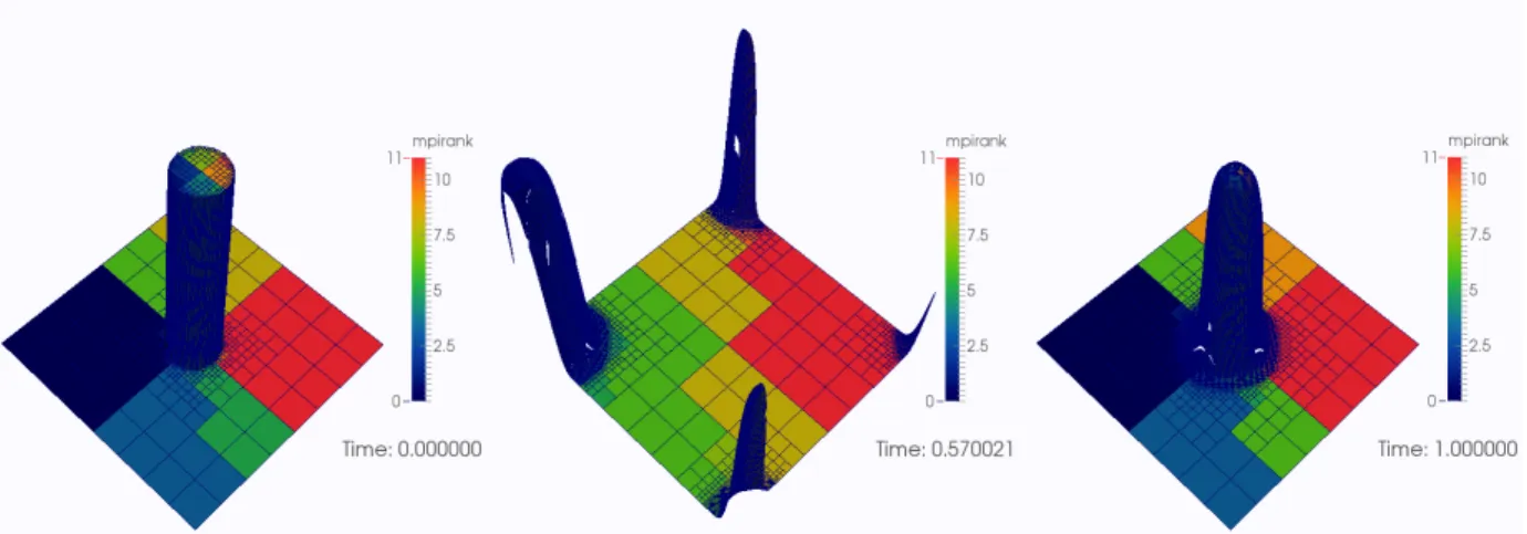
We consider again the transport problem at constant pressure and constant velocity of section 4.1 with a sharp profile of volume fraction defined by α0pxq “ 1 ´ λ if |x ´ x0| ă 0.1, α0pxq “ λ otherwise. The domain is periodic. AMR is governed by the ρ-gradient criterion with the same refinement threshold as in the 4.1 case. Figure 4 shows the resulting profiles obtained with the MUSCL-Hancock scheme at several instants with a color representation of the 12 MPI processes domain decomposition. The refinement criterion and the 2:1 balance property are well-managed by p4est.

4.2.1. Adapted versus uniform meshes

In this section we compare results obtained with uniform grids and adapted meshes in order to assess the ability of the AMR procedure to act as a compression technique, preserving accuracy while decreasing the computational needs. In the following, ∆xminis the space step of the reference uniform mesh. It is equal to the size of the most refined cell in the AMR simulation and it is fixed for a series of simulation. On the other hand ∆xmax is the largest allowed space step for the AMR simulation. It varies from ∆xmin to 26∆xmin, so

Figure 4. View of the adaptive meshing and domain decomposition, load-balancing and 2:1 balance for the disk advection test case. ∆xmax“ 2´3, ∆xmin“ 2´8. 2nd-order MUSCL-Hancock scheme.

(a) ξ “ 5 ˆ 10´4 (b) ξ “ 5 ˆ 10´5

Figure 5. L1-error versus level of compression of the mesh. Each compressed mesh is compared with its equivalent uniform mesh (log₂p∆xmaxq ´ log2p∆xminq “ 0) given in the same color. The study is lead for two different values of the threshold ξ for ρ-gradient refinement criterion.

that the so called level of compression, log2p∆xmaxq ´ log2p∆xminq varies from 0 to 6. The second order scheme and the ρ-gradient refinement criterion have been used to perform the different simulations.

Figure 5 shows the evolution of the L1-error with the level of compression for two different values of the refinement threshold ξ. There, we see that for too large a refinement criterion, the compression error may prevail over the scheme consistency error when the space step ∆xmingoes to zero. This can be seen in Figure 5a for ∆xmin “ 2´9 and ∆xmin“ 2´10 (red and blue lines), where the L1 errors of the compressed meshes are significantly higher than the L1 _{error of the equivalent uniform mesh and do not seem to decrease with} finer ∆xmin. However, decreasing the threshold ξ for the refinement criterion enables to recover the expected accuracy of the compressed simulations, as shown in Figure 5b. Then, there exists a subtle equilibrium for the refinement criterion: too small a value implies refinement everywhere and cancelation of the advantages of the AMR technique, whereas too large a value makes the compression error so large that mesh convergence is lost.

When the refinement criterion is sufficiently small, the accuracies of the uniform and AMR solutions are comparable, and the computational time on the compressed mesh is indeed better. This is illustrated in

(a) At a fixed highest level of refinement ∆xmin, we

pare the total CPU time (full line and marks) and com-pression rates (dashed lines) of the uniform mesh (in black) and the meshes with 1, 2 and 6 levels of compression (∆xmax“ 21,2 or 6∆xmin). Performed on 1 MPI process.

(b) Mean computation times (total time, time spent in finite volume solver and time for mesh management) per quadrant, for different problem sizes but with a same amount of work per process (weak scaling).

Figure 6. Adaptive mesh resolution and computational costs

Figure 6a. This figure also displays the resulting compression rate, namely the ratio between the number of cells in the compressed mesh and in the equivalent uniform mesh. However, due to the rather large level of diffusion in the α-advection test case, the compression rate is not as high as expected. We think that a less diffusive numerical scheme would enlarge uniform regions and therefore improve the AMR efficiency, needed for example in the case of the dynamics of a sharp interface between two phases. Anyway, even though the AMR technique brings a certain overload for the management of the non-uniform mesh, the high compression rate allows an overall gain in terms of CPU time.

4.2.2. Parallel performance

In this section, we present few cases testing some aspects of the parallel performance. Nonetheless, we need to emphasize that the code here is a raw first version that did not benefit from any optimization. It may be significantly improved in term of computational efficiency.

Strong scaling

We use our α-profile transport test with a number of MPI processes ranging from 1 to 96. The runs are set in order to preserve the total number of cells approximately equal to 4.6 ˆ 106 _{cells. Figure 7a allows} to evaluate the resulting speed-ups: for a low number of MPI processes the speed-up is very close to 1. However, in our case, for greater numbers of processes, the number of cells handled by the solver in each process is not sufficient to match the communication cost that becomes predominant. Indeed, as shown in Figure 4, the domain decomposition by even split of the z-curve does not always provide convex domains (some are not even connected). Therefore, the more MPI processes involved, the more the domain space is

(a) Strong scaling of total time of computation, of solver resolution and of mesh adaptation algorithms for about 4.6 ˆ 106cells.

(b) Repartition of the computational time among the main tasks of the code according to meshes of different sizes and compression rates. 24 MPI-processes were used.

Figure 7. Strong scaling and time repartition for the α-advection simulation.

fragmented and the ratio of cells at the frontiers of each subdomain by its total number of cells increases, and so does the communications between the subdomains.

Basic code profiling

We perform an elementary profiling analysis in order to compare the CPU time allocated to the adaptation process versus the time spent in the Finite Volume solver given meshes that are successively refined, thus increasing their number of cells, for a fixed number of 24 MPI processes. In Figure 7b we display different tasks identified in the code. We can see that the part dedicated to the mesh management given by the seven first colors (from light pink to dark red) decreases when the number of cells in the mesh increases. In particular, the part dedicated to the 2:1 balancing task, the longest one, is significantly reduced.

To sum up, Figures 7a and 7b show that p4est has good computation efficiency for important enough work loads, i.e. for a high number of cells in the mesh. When the work load of each process is too low, an excessive time seems to be spent in communications between the processes compared to the time spent in the solver.

Weak scaling

We now evaluate the evolution of the computational time when increasing the number of working processes at a constant workload (see Figure 6b). We maintain a number around 1.2 ˆ 104 _{cells (the number of cells} changes during the computation due to diffusion) managed by each process by increasing the global number of cells. The times of computation per quadrant are averaged over the 1000 first time steps. While we did not succeed in preserving an exactly constant computational time per quadrant, the results are good and agree with similar results already obtained in [9].

4.3. 2D and 3D gravity driven two-phase flows

In this section, we take the gravity source term S “ p0, 0, 0, ´ρg, 0qT _{into account by adding an additional} operator l∆t{2S in our splitting sequence (5) or (10), following standard lines. For a given discrete state ĂWi We set l∆t{2S WĂi “ rρri, ĆpρY qi, Čpρuxqi, Čpρuyq_i´ρrig∆t{2, Ćpρuzqis. For three-dimensional problems, the overall

Figure 8. Simulation of a liquid drop falling onto a free surface with the refinement criterion α-gradient. Mapping of the volume fraction α.

splitting strategy becomes:

l∆t{2X l ∆t{2 Y l ∆t{2 S l ∆t{2 Z l ∆t{2 Z l ∆t{2 Y l ∆t{2 S l ∆t{2 X .

We emphasize that the following tests aim at assessing the overall behavior of the code. While the physical behavior of the solutions is roughly correct, a more careful setup and systematic comparison with physical observations are still to be conducted in order to obtain a thorough validation.

2D bubble drop test

We consider the simulation of a falling drop of liquid (fluid 2) surrounded by a gas (fluid 1) toward a resting free surface separating a liquid bath from the gas. At t “ 0, we suppose that ρ1“ 1.0pkg{m3q and ρ2“ 1.0 ˆ 103pkg{m3q. We use solid wall boundary conditions.

We choose to use the α-gradient refinement criterion, with ξ “ 5ˆ10´4_{in order to refine the mesh mainly} in the vicinity of the gas/liquid interface. The simulation is performed on a mesh with a minimum refining level of 3 and maximum of 9. Using 48 MPI processes, the time of computation is about 15 minutes on the computing Mesocenter of Ecole Centrale Paris, which is an Altix ICE 8400 LX. Each node is composed of two six-core Intel Xeon X5650 processors. Figure 8 provides the mapping of the computed α at several instants along with the adapted mesh. The mesh hits the finest refinement level in the vicinity of the interface where gradients of α are strong. Due to the numerical diffusion, we see that far from the interface gradients of α are detected and the mesh is also refined.

3D dam break test

The second gravity-driven flow considered here deals with the evolution of a free surface in a dam break situation. This problem has been studied in many works featuring simulations and experiments (see e.g. [5, 39]). We show in Figure 9 the results of a 3D simulation. The computation was performed on 64 nodes of 8 CPU cores each of the computing Mesocenter of Centrale Paris. A physical time of 1.5s has been reached: typically, given our initial conditions, the flow of liquid reaches the opposite side of the domain within 0.3s and a second wave comes back within 1s. The whole computation took about 4h for 5.59 ˆ 105 _iterations. The highest level of refinement is 8 and the lowest 3. At the beginning of the simulation, the number of cells was 5.88 ˆ 104 _{(3.5 ˆ 10}´3 _{compression rate), at the end, due to diffusion and acoustic effects, it reached} 1.25 ˆ 106 _{(7.4 ˆ 10}´2 _{compression rate), while the equivalent uniform mesh would have around 1.7 ˆ 10}7 cells.

The refinement criterion is still α-gradient and leads to an affordable computational cost, whereas the resolution of the problem on the finest grid would require a much longer time as well as a much larger memory. The volume fraction iso-surface α ă 0.5, standing for the liquid phase, as well as the mesh at the domain boundaries are represented in the subfigures of Figure 9 at several time steps. At time t “ 0, both fluids are still. Due to gravity, the liquid flows into the chamber. These results are very encouraging, even if they require further validation, as already stated, and if the influence of the refinement criterion on the dynamics of the solution has to be studied carefully.

5. Conclusion and perspectives

The AMR library p4est brings solutions to some issues for tree-based AMR, ranging from mesh and data structure using linear arrays, to cache locality thanks to the interesting properties of the z-order curve, and parallel efficiency through load balancing. Understanding the main functionalities of p4est and testing its ease of use and basic performance were the main objectives of the six weeks of CEMRACS 2014. Within this framework, we have achieved a first version of a code, using a finite volume scheme of the relaxation type, at first and second order in space and time, applied to a simple but representative two-fluid two-phase flow model. The scheme has been verified through classical test cases (advection, shock tube, double rarefaction) and a convergence analysis has been conducted.

Some very promising simulations in 2D and 3D have been achieved and the code possesses all the good features in terms of parallel efficiency and accuracy, which allow both conducting reasonable size computa-tions within a short amount of time (typically on a Mesocenter type of machine where the AMR strategy and its implementation lead to a solution at the same level of accuracy as uniform meshes but with significant savings in computational cost and memory requirement), and envisioning large scale and efficient simulations on larger massively parallel machines. Such conclusions can be drawn, even if the tool requires both further optimization and detailed and thorough study in terms of validation and accuracy of refinement criteria for the two-phase test-cases under study.

Let us also underline that there are some issues, which were not tackled in the present study. Among them, the problems we have studied do not involve a very large spectrum of time scales in terms of the dynamics of the problem [19] and the issue of local time stepping/multi-scale treatment will require some effort. Higher order numerical method will also require adapting the strategy proposed in the paper, as well as solving for elliptic equations such as in plasma physics and low speed flows (Low Mach approximation or incompressible flows). Such issues, even if interesting, were out of reach during the time of the project.

Acknowledgement

The support of EM2C laboratory and of Maison de la Simulation for the CEMRACS project are gratefully acknowledged. The Ph.D. of F. Drui is funded by a CEA/DGA (Direction Générale de l’Armement - French Department of Defense) grant. The use of the computational Mesocenter of Ecole Centrale Paris for some of the simulations is also gratefully acknowledged.

References

[1] M. Adams, P. Colella, D. T. Graves, J.N. Johnson, N.D. Keen, T. J. Ligocki. D. F. Martin. P.W. McCorquodale, D. Modi-ano. P.O. Schwartz, T.D. Sternberg, and B. Van Straalen. Chombo software package for amr applications - design document. Lawrence Berkeley National Laboratory Technical Report, 2013.

Figure 9. Simulation of a dam break. View of mesh and volume fraction α ă 0.5. Refinement criterion is α-gradient.

[2] M. Bergdorf and P. Koumoutsakos. A Lagrangian particle-wavelet method. Multiscale Model. Simul., 5(3):980–995, 2006. [3] M. J. Berger and P. Collela. Local adaptive mesh refinement for shock hydrodynamics. Journal of Computational Physics,

82(1):64–84, 1989.

[4] M. J. Berger and J. Oliger. Adaptive mesh refinement for hyperbolic partial differential equations. Journal of Computational Physics, 53(3):484–512, 1984.

[5] A. Bernard-Champmartin and F. De Vuyst. A low diffusive lagrange-remap scheme for the simulation of violent air–water free-surface flows. Journal of Computational Physics, 274(0):19 – 49, 2014.

[6] C. Berthon. Why the muscl-hancock scheme is L1_{-stable. Numerische Mathematik, 104:27–46, 2006.}

[7] F. Bouchut. Nonlinear Stability of Finite Volume Methods for Hyperbolic Conservation Laws and Well-Balanced Schemes for Sources. Birkhäuser, 2004.

[8] K. Brix, S. S. Melian, S. Müller, and G. Schieffer. Parallelisation of multiscale-based grid adaptation using space-filling curves. In ESAIM: Proceedings, volume 29, pages 108–129. EDP Sciences, 2009.

[9] C. Burstedde, L. C. Wilcox, and O. Ghattas. p4est: Scalable algorithms for parallel adaptive mesh refinement on forests of octrees. SIAM Journal on Scientific Computing, 33(3):1103–1133, 2011.

[10] F. Caro, F. Coquel, D. Jamet, and S. Kokh. A simple finite-volume method for compressible isothermal two-phase flows simulation. International Journal of Finite Volume, 3(1), 2006.

[11] C. Chalons and J.-F. Coulombel. Relaxation approximation of the Euler equations. J. Math. Anal. Appl., 348(2):872–893, 2008.

[12] G. Chanteperdrix, P. Villedieu, and J.P. Vila. A compressible model for separated two-phase flows computations. In ASME Fluid Eng. Div. Summer Meeting 2002, 2002.

[13] P. Chatelain, G.-H. Cottet, and P. Koumoutsakos. Particle mesh hydrodynamics for astrophysics simulations. Internat. J. Modern Phys. C, 18(4):610–618, 2007.

[14] A. Cohen, S. M. Kaber, S. Müller, and M. Postel. Fully adaptive multiresolution finite volume schemes for conservation laws. Mathematics of Computation, 72:183–225, 2003.

[15] F. Coquel, Q.L. Nguyen, M. Postel, and Q.H. Tran. Local time stepping applied to implicit-explicit methods for hyperbolic systems. Multiscale Model. Simul., 8(2):540–570, 2009/10.

[16] G.-H. Cottet and P. D. Koumoutsakos. Vortex methods. Cambridge University Press, Cambridge, 2000. Theory and practice.

[17] S. Descombes, M. Duarte, T. Dumont, , T. Guillet, V. Louvet, and M. Massot. Task-based adaptive resolution of time-space multi-scale reaction-diffusion systems on multi-core shared memory architectures. SIAM Journal on Scientific Computing, pages 1–24, 2015. Submitted - Available on HAL https://hal.archives-ouvertes.fr/hal-01148617.

[18] M. Duarte. Adaptive numerical methods in time and space for the simulation of multi-scale reaction fronts. Thèse, Ecole Centrale Paris, December 2011. https://tel.archives-ouvertes.fr/tel-00667857.

[19] M. Duarte, S. Descombes, C. Tenaud, S. Candel, and M. Massot. Time-space adaptive numerical methods for the simulation of combustion fronts. Combustion and Flame, 160(6):1083–1101, 2013.

[20] M. Duarte, M. Massot, S. Descombes, C. Tenaud, T. Dumont, V. Louvet, and F. Laurent. New resolution strategy for multiscale reaction waves using time operator splitting, space adaptive multiresolution, and dedicated high order implicit/explicit time integrators. SIAM J. Sci. Comput., 34(1):A76–A104, 2012.

[21] A. Dubey, A. Almgren, J. Bell, M. Berzins, S. Brandt, G. Bryan, P. Colella, D. Graves, M. Lijewski, F. Löffler, B. O’Shea, E. Schnetter, B. Van Straalen, and K. Weide. A survey of high level frameworks in block-structured adaptive mesh refinement packages. Journal of Parallel and Distributed Computing, 74(12):3217 – 3227, 2014. Domain-Specific Languages and High-Level Frameworks for High-Performance Computing.

[22] A. Harten. Multiresolution algorithms for the numerical solution of hyperbolic conservation laws. Comm. Pure and Applied Math., 48:1305–1342, 1995.

[23] T. Isaac, C. Burstedde, and O. Ghattas. Low-cost parallel algorithms for 2:1 octree balance. In Parallel Distributed Processing Symposium (IPDPS), 2012 IEEE 26th International, pages 426–437, May 2012.

[24] H. Ji, F.-S. Lien, and E. Yee. A new adaptive mesh refinement data structure with an application to detonation. Journal of Computational Physics, 229(23):8981–8993, November 2010.

[25] A. M. Khokhlov. Fully threaded tree for adaptive refinement fluid dynamics simulations. Journal of Computational Physics, 143(2):519–543, July 1998.

[26] P. Koumoutsakos. Multiscale flow simulations using particles. In Annual review of fluid mechanics. Vol. 37, volume 37 of Annu. Rev. Fluid Mech., pages 457–487. Annual Reviews, Palo Alto, CA, 2005.

[27] R. J. Leveque. Finite-Volume Methods for Hyperbolic Problems. Cambridge University Press, 2004.

[28] J. J. Monaghan. Smoothed particle hydrodynamics. Annual Review of Astronomy and Astrophysics, 30:543–574, 1992. [29] S. Müller. Adaptive Multiscale Schemes for Conservation Laws, volume 27. Springer, 2003. Ed. T. J. Barth, M. Griebel,

D. E. Keyes, R. M. Nieminen , D. Roose and T. Schlick.

[30] S. Müller and Y. Stiriba. Fully adaptive multiscale schemes for conservation laws employing locally varying time stepping. J. Sci. Comput., 30(3):493–531, 2007.

[31] S. Popinet. Gerris: a tree-based adaptive solver for the incompressible euler equations in complex geometries. Journal of Computational Physics, 190(2):572–600, September 2003.

[32] D. Rossinelli, B. Hejazialhosseini, D. G. Spampinato, and P. Koumoutsakos. Multicore/multi-GPU accelerated simulations of multiphase compressible flows using wavelet adapted grids. SIAM J. Sci. Comput., 33(2):512–540, 2011.

[33] I. Suliciu. On modelling phase transitions by means of rate-type constitutive equations, schock wave structure. International Journal of Engineering Science, 1:829–841, 1990.

[34] R. Teyssier. Cosmological hydrodynamics with adaptive mesh refinement. a nex high resolution code called ramses. Astronomy and Astrophysics, 385:337–364, 2002.

[35] E. F. Toro. Riemann Solvers and Numerical Methods for Fluid Dynamics - A Practical Introduction. Springer, 3rd edition, 2009.

[36] E.F. Toro, M. Spruce, and W. Speares. Restoration of the contact surface in the HLL-Riemann solver. Shock Waves, 4(1):25–34, 1994.

[37] B. van Leer. On the relation between the upwind-differencing schemes of godunov, engquist-osher and roe. SIAM Journal on Scientific and Statistical Computing, 5(1):1–20, 1984.

[38] A. B. Wood. A textbook of Sound. The Macmillan Company, 1930.

[39] X.-Z. Zhao. Validation of a cip-based tank for numerical simulation of free surface flows. Acta Mechanica Sinica, 27(6):877– 890, 2011.