Regime switching model for financial data: empirical risk analysis

HAL Id: hal-01095299

https://hal.inria.fr/hal-01095299v2

HAL is a multi-disciplinary open access

archive for the deposit and dissemination of sci-entific research documents, whether they are pub-lished or not. The documents may come from teaching and research institutions in France or abroad, or from public or private research centers.

L’archive ouverte pluridisciplinaire HAL, est destinée au dépôt et à la diffusion de documents scientifiques de niveau recherche, publiés ou non, émanant des établissements d’enseignement et de recherche français ou étrangers, des laboratoires publics ou privés.

Regime switching model for financial data: empirical

risk analysis

Khaled Salhi, Madalina Deaconu, Antoine Lejay, Nicolas Champagnat,

Nicolas Navet

To cite this version:

Khaled Salhi, Madalina Deaconu, Antoine Lejay, Nicolas Champagnat, Nicolas Navet. Regime switch-ing model for financial data: empirical risk analysis. Physica A, Elsevier, 2016, 461, pp.148-157. �10.1016/j.physa.2016.05.002�. �hal-01095299v2�

Regime switching model for financial data: empirical

risk analysis

Khaled Salhi

Madalina Deaconu

Antoine Lejay

Nicolas Champagnat

Nicolas Navet

June 1, 2016

Abstract

This paper constructs a regime switching model for the univariate Value-at-Risk estimation. Extreme value theory (EVT) and hidden Markov models (HMM) are combined to estimate a hybrid model that takes volatility clustering into account. In the first stage, HMM is used to classify data in crisis and steady periods, while in the second stage, EVT is applied to the previously classified data to rub out the delay between regime switching and their detection. This new model is applied to prices of numerous stocks exchanged on NYSE Euronext Paris over the period 2001-2011. We focus on daily returns for which calibration has to be done on a small dataset. The relative performance of the regime switching model is benchmarked against other well-known modeling techniques, such as stable, power laws and GARCH models. The empirical results show that the regime switching model increases predictive per-formance of financial forecasting according to the number of violations and tail-loss tests. This suggests that the regime switching model is a robust forecasting variant of power laws model while remaining practical to implement the VaR measurement.

Keywords: Value-at-Risk; power tail distribution; Hidden Markov Model; regime switch-ing.

1

Introduction

The Value-at-Risk (VaR) is one of the main risk indicators for management of financial portfolios [32]. It is the threshold above which a loss over a chosen time horizon occurs with at most a given level of confidence.

The VaR may be estimated either by parametric or non-parametric techniques. The non-parametric ones use only the empirical distributions (historical, resampling) without

a _{Université de Lorraine, Institut Elie Cartan de Lorraine, UMR 7502, Vandoeuvre-lès-Nancy, F-54506,}

France.

b_{CNRS, Institut Elie Cartan de Lorraine, UMR 7502, Vandoeuvre-lès-Nancy, F-54506, France.}

c_{Inria, Villers-lès-Nancy, F-54600, France.}

d _{FSTC/CSC Research Unit/Lassy lab., Université du Luxembourg, L-1359 Luxembourg.}

† _{Email: tKhaled.Salhi,Madalina.Deaconu,Antoine.Lejay,Nicolas.Champagnatu@inria.fr}

fitting a model. Due to the small amount of available data, it does not provide an accurate estimate for the probability of extreme events. The parametric approach overrides partly the problem induced by the lack of data by fitting the parameters of a model on historical data and computing afterwards the VaR, either by analytical or numerical methods.

The RiskMetric methodology [41] is widely used to estimate the risk associated to a portfolio by establishing quantitative relations between variations of the risk indicator with respect to risk factors (stocks and prices of derivatives for example). Nowadays this methodology incorporates heavy tail distributions, but it was initially developed in the Gaussian context, which is still prevalent in risk management and enforced by Basel Accord [50].

However, actual regulations and standard procedures for computing the VaR, based mainly on the Gaussian world, have been invalidated by many studies (see e.g. [1, 6]) as they strongly underestimate the extreme events observed in the market.

The successive financial crises since 1987 led to a greater attention in modeling tail behavior of the induced returns distributions, and to the use of Extreme Value Theory (EVT) as a central concept in Risk Management [21].

Neither single model nor statistical methodology is acknowledged as standard for deal-ing with heavy-tails. In this study, we construct a variant of power law tails of the dis-tributions by taking into consideration the regime switching between crisis and steady periods. We compare our model to several known models (stable, Generalized Pareto tails of distribution and GARCH). We consider heavy tail distributions for the losses 𝐿 with distribution function 𝐹 , typically, generalized Pareto (power laws):

1 ´ 𝐹 p𝑥q “ Pp𝐿 ě 𝑥q “ ℓp𝑥q

𝑥𝛼 , (1)

where ℓ is a function of slow variation and 𝛼 is the tail index which summarizes the heaviness of the tail distribution and characterizes also the existence of moments.

In our approach, we aim to benefit from the stability of power law models in the VaR forecasting and the detection of volatility clustering given by conditional models. We assume the existence of two states: crisis and steady, and we classify data in two regimes using hidden Markov models (HMM). Then, the power law tail distribution is estimated from the past crisis and steady periods. The model gives more weight to the current regime, which reduces under-estimations and over-estimations at the beginning of crisis and steady periods.

We focus here only on univariate distributions. The case of several stocks leads to higher complexity, as the notion of VaR itself is not properly defined (see e.g. [47]). The multivariate case will be subject of further studies.

Our models of risk are intensively tested on historical market data from NYSE Eu-ronext Paris. We focus only on daily returns of single stock prices, which is the practical situation of small investors and for which the problem of model calibration is the most difficult because of the small amount of data.

Outline. In Section 2, we give an overview of heavy-tailed models used in finance, the markets on which they have been applied and the estimators for power laws. In Section 3, we introduce our methodology for estimating the parameters and performing the backtesting. Finally, in Section 4, we introduce our dataset and discuss the conclusions we draw from the study over a selection of 56 stocks from NYSE Euronext Paris. Perspectives and conclusions are then highlighted in Section 5.

2

Empirical evidence for heavy tails

2.1 Evidences for the power law in financial markets

It is widely acknowledged that prices and returns of stocks obey to general laws usu-ally called “stylized facts” [16]. Skewness and heavy-tail are the two main properties of observed prices which are not verified by the Black&Scholes models.

Although stable distributions have been proposed since the 60’s [24, 38] and an alter-native model (finite variance subordinated log-normal distributions) has been proposed in 1973 by P. Clark [15], the systematic use of Extreme Value Theory (EVT) is recent, as the crash of 1987 urged for a better understanding of large losses. For early occurrences of the use of EVT focusing only on the tail distributions, let us cite [31, 35, 36].

Developed markets have been investigated as well, mainly through market indices: S&P 500, Dow Jones and Nasdaq [37], German DAX Stocks [22], Australian ASX-ALL [49], Nikkei and Eurostoxx 50 [28], etc.

Stable distributions and processes exhibit generalized Pareto tail distributions as in (1). Yet, choosing this model imposes tail index 𝛼 ă 2. This parameter is difficult to estimate, especially when close to 2 [23]. Many critical studies (see e.g. [23, 53]) show that the tail index is greater than 2, and around 3 for short terms returns.

To estimate the generalized Pareto distribution, let us consider that the return 𝑋 at a given time satisfies (1) and that 𝑛 successive returns p𝑋1, . . . , 𝑋𝑛q are independent or

at least stationary. It is a crucial and complex problem to estimate 𝛼 and ℓp𝑥q written in a parametric or semi-parametric form (for example, ℓp𝑥q “ 𝐶 or ℓp𝑥q “ 𝐶1` 𝐶2𝑥´𝛽`

op𝑥´𝛽

q), as well as the threshold 𝑥0above which the previous expressions for ℓp𝑥q are valid.

For studying the tail of the distribution of 𝑋, we use order statistics p𝑋p1q, . . . , 𝑋p𝑛qq of

p𝑋1, . . . , 𝑋𝑛q with 𝑋p1q ď 𝑋p2q ď ¨ ¨ ¨ ď 𝑋p𝑛q.

A large family of estimators is available but none of them supersedes the others. For our purposes, we adopt the Hill estimator defined by

𝐻𝑘,𝑛 “ 1 𝑘 𝑘 ÿ 𝑗“1 ln 𝑋p𝑛´𝑗`1q´ ln 𝑋p𝑛´𝑘q (2)

as an estimator of 𝛾 “ 1{𝛼. There are several ways to interpret this estimator (maximum likelihood, least squares...). The main difficulty for its implementation consists in choosing the optimal index 𝑘. We refer to the book [5] and references therein.

2.2 Commonly used models for heavy tails

Many studies have looked for alternatives to power laws modeling. There is a huge literature on this subject [44], and we give here the main lines with a focus on univariate returns. Regarding stochastic processes in continuous time, various authors considered jump diffusion models [17], variance Gamma processes [39] and subordinated processes [15], and SDE whose invariant distributions are fat-tailed [42, 48] or present moments explosions [29, Chapter 7].

Chronological series play also a very important role in the development of such financial models for stock prices. A large class of models assumes that the returns are solutions to equations of the form 𝑟𝑡`1 “ 𝜇𝑟𝑡` 𝜎𝑡𝜀𝑡, where 𝜎𝑡 is itself described by an equation of

similar form, leading to General Autoregressive Conditional Heteroskedasticity (GARCH) models which capture clustering effects in volatility. Here, the innovation 𝜀𝑡 is a noise,

that could be Gaussian or follow other distributions like Student’s 𝑡 distributions [18]. A quantitative manifestation of volatility clustering is that, while returns themselves are

uncorrelated, absolute returns |𝑟𝑡| or their squares display a positive, significant and slowly

decaying autocorrelation function corrp|𝑟𝑡|, |𝑟𝑡`𝜏|q ą 0 for 𝜏 ranging from a few minutes to

several weeks. However, in terms of extreme values, several studies, in different financial markets, concluded that the quantile forecasting performance of power law models is better than that of GARCH type models [14, 26, 27, 33]. GARCH models yield volatile quantile forecasts, while power laws lead to more stable ones. A detailed examination of the VaR forecasts from these two classes of models proved that wild swings observed in the GARCH VaR predictions are more an artifact of the GARCH model, rather than the underlying data [19].

Finally, another approach consists in separating the tail of the distribution from its bulk through hybrid models. Several approaches may be found in [45]. Furthermore, mixtures of models may also lead to heavy tails [10].

3

Framework and methodology

3.1 Log returns and Value-at-Risk

Let 𝑅𝑡 “ ln p𝑆𝑡`1{𝑆𝑡q be the (log-)return, or more simply the return, at time 𝑡 where 𝑆𝑡

is the price of a stock at time 𝑡. We call losses the values 𝐿𝑡 “ ´𝑅𝑡. The daily VaR𝑡p𝑎q

at level 𝑎 P p0, 1q is defined by

1 ´ 𝑎 “ Pp𝑅𝑡ă VaR𝑡p𝑎qq (3)

which represents the quantile 𝑞𝑅

1´𝑎 at level p1 ´ 𝑎q of the returns distribution (or the

quantile 𝑞𝐿

𝑎 at level 𝑎 of the losses distribution).

After having fixed a class of parametric models, the practical computation of the VaR consists in calibrating the parameters for the common distribution of 𝑅 or 𝐿 (actually only its tail) and computing the quantile 𝑞𝑅

1´𝑎 or 𝑞𝑎𝐿.

3.2 Models

We consider four classes of parametric univariate models for the returns or losses: (I) The stable distribution for the returns defined by its characteristic function

𝜑𝑋p𝑡q “

#

expr𝑖𝜇𝑡 ´ 𝜎𝛼_|𝑡|𝛼_{p1 ´ 𝑖𝛽 signp𝑡q tanp}𝜋𝛼

2 qqs if 𝛼 ‰ 1,

expr𝑖𝜇𝑡 ´ 𝜎|𝑡|p1 ` _𝜋2𝑖𝛽 signp𝑡q ln |𝑡|qs if 𝛼 “ 1, (4) where 𝛼 P p0, 2q is the tail index, 𝛽 P p´1, 1q is the skewness, 𝜎 ě 0 is the scale parameter and 𝜇 P R the location parameter (see e.g. [25, 43]). Stable distributions arise naturally as universal classes when looking to limit theorems.

(II) The Pareto distribution for tails of the losses gives for the distribution function of the returns,

Pp𝐿𝑡 ě 𝑥q “ 𝐶 𝑥´𝛼 for 𝑥 ě 𝑥0. (5)

This model does not make any supplementary assumption on the bulk of the distribution of the returns.

Except for 𝛼 “ 2, where stable distributions are Gaussian, the parameter 𝛼 of stable laws corresponds to their Pareto tail index, with ℓp𝑥q converging to a constant [43, Theo-rem 1.12]. Pareto distributions offer a wider variety of fat tails by Theo-removing the constraint 𝛼 ă 2.

(III) The GARCH-𝑡 model. We consider the GARCH p1, 1q model for the time series of financial returns. More precisely, suppose p𝑅𝑡q satisfies the following model :

𝑅𝑡“ 𝜇 ` 𝜀𝑡 “ 𝜇 ` 𝜎𝑡𝑍𝑡, (6)

𝜎2_𝑡 “ 𝜔 ` 𝛼𝜀2<sub>𝑡´1</sub>` 𝛽𝜎2_𝑡´1, (7) where p𝑍𝑡q is a sequence of i.i.d. Student-𝑡 innovations. Our choice for Student-𝑡

innova-tions is based on many studies showing that Student-𝑡 innovainnova-tions give the best GARCH fitting performance [18].

(IV) The regime switching model. The VaR forecasting under the assumption of Pareto distribution shows a clustering of under-estimations (respectively over-estimations) at the beginning of each period of large (respectively small) fluctuations (see Fig. 3). The interpretation is that, after a regime switching, we estimate the VaR with data from the other regime. Therefore, we construct a regime switching model that considers a mixture of Pareto distribution. These regime switching models suppose the existence of a state process that is at the origin of the returns. This process is generally chosen as being a markov chain. Many authors use logistic functions of lagged endogenous variables [2, 30], probabilistic functions [46] or Hamilton filter [7] to construct the state chain. These methods are based on an a priori knowledge of the transition probabilities. In our methodology, we are looking to use the a priori knowledge as less as possible. So, we introduce a Hidden Markov Model (HMM) that represents an unsupervised learning procedure from data. We suppose that the return 𝑅𝑡 at time 𝑡 depends on a hidden state

𝑋𝑡, which can take 2 values 𝑐 and 𝑠 corresponding to crisis (𝑋𝑡“ 𝑐, large fluctuations) or

steady (𝑋𝑡“ 𝑠, small fluctuations) periods.

HMM has been first proposed by L. E. Baum and his co-authors [3, 4] in the late 60’s. These models assume the existence of a non-observed variable that is the source of obser-vations, and try to estimate the hidden variable. This hidden variable 𝑋𝑡 is supposed to

be a Markov chain. The model is fully characterized by the parameters 𝑀 “ p𝜌, 𝑄, 𝜓q of the HMM:

(i) the initial law 𝜌 of 𝑋:

𝜌p𝑥q “ Pp𝑋0 “ 𝑥q, 𝑥 P t𝑐, 𝑠u,

(ii) the transition matrix 𝑄 of 𝑋: 𝑄p𝑥, 𝑥1

q “ Pp𝑋𝑡`1“ 𝑥1|𝑋𝑡 “ 𝑥q, 𝑥, 𝑥1 P t𝑐, 𝑠u, @𝑡 ě 0,

(iii) the emission kernel of 𝑅 given 𝑋:

𝜓p𝑥, 𝑑𝑦q “ Pp𝑅𝑡P 𝑑𝑦|𝑋𝑡“ 𝑥q, 𝑥 P t𝑐, 𝑠u, 𝑦 P R, @𝑡 ě 0,

where 𝜓p𝑥, ¨q is a probability measure on R. The model of losses tails is then given by

Pp𝐿𝑡 ě 𝑥q “ Pp𝐿𝑡ě 𝑥|𝑋𝑡“ 𝑐qPp𝑋𝑡“ 𝑐q ` Pp𝐿𝑡 ě 𝑥|𝑋𝑡“ 𝑠qPp𝑋𝑡“ 𝑠q

“ 𝐶𝑐𝑥´𝛼𝑐 Pp𝑋𝑡 “ 𝑐q ` 𝐶𝑠𝑥´𝛼𝑠 p1 ´ Pp𝑋𝑡“ 𝑐qq

(8)

for 𝑥 ě 𝑥0, where p𝐶𝑐, 𝛼𝑐q and p𝐶𝑠, 𝛼𝑠q are respectively the Pareto distribution parameters

of crisis and steady losses. The parameters 𝑀 “ p𝜌, 𝑄, 𝜓q, 𝐶𝑐, 𝛼𝑐, 𝐶𝑠, 𝛼𝑠 and Pp𝑋𝑡 “ 𝑐q

3.3 Parameters estimation and computation of the VaR

We make the hypothesis that the series of stock prices p𝑆𝑡q𝑡 is stationary over the time

(models I and II), p𝜎𝑡q𝑡 is time homogeneous (model III), or the HMM p𝑋𝑡, 𝑅𝑡q𝑡 is time

homogeneous (model IV). For the first two models, we adopt a moving window approach with a window size of 252 days (one year of data). For instance, the window is placed between the first and 252nd days and a given quantile is forecast for the 253rd day. Next, the window is slid one step forward to forecast quantiles for the 254th, 255th, ..., last days. The motivation behind the moving window technique is to capture dynamic time-varying characteristics of the data in different time periods and to emulate the situation where a small investor wants to forecast the VaR for the next day. The GARCH approach is not based on a moving window but uses all the available data up to the day on which forecasts are generated. This approach is preferable since the detection of volatility clustering requires more data. The last model uses a window composed from 252 crisis data and 252 steady periods data as explained in (IV). We proceed as follows:

(I) Stable Distribution. For the stable distribution, we use for the returns the Mc-Culloch method [40] as implemented in the R library fBasics on the data p𝑅1, . . . , 𝑅𝑛q to

estimate the four parameters 𝛼, 𝛽, 𝜎 and 𝜇 and to compute the quantile through a direct estimation of the distribution function.

(II) Pareto distribution. We use a slight modification of the Hill estimator. Let p𝐿p1q, . . . , 𝐿p𝑛qq be the increasing order statistics of p𝐿1, . . . , 𝐿𝑛q whose common

distribu-tion is assumed to satisfy Pp𝐿1 ě 𝑥q “ 𝐶𝑥´𝛼 for 𝑥 ě 𝑥0.

Then, if one writes

ln 𝐿p𝑖q “ ´𝛾 ln

ˆ 𝑛 ` 1 ´ 𝑖 𝑛 ` 1

˙

` 𝐾 ` 𝜀𝑖, (9)

where 𝛾 “ 1{𝛼 and 𝐾 “ 𝛾 ln 𝐶, the noise 𝜀𝑖 is small for 𝑛 and 𝑖 large enough. Plotting

ln 𝐿p𝑖q as a function of ´ lnpp𝑛 ` 1 ´ 𝑖q{p𝑛 ` 1qq gives the Pareto plot which should be close

to linear for large 𝑖. The Hill estimator (2) computes the slope of this graph using weighted least squares. For more stability, we remove the highest values. We set 𝑑𝑛 “ t0.95 ˆ 𝑛u,

𝑢𝑛 “ t0.99 ˆ 𝑛u and we use ˆ𝛾 as an estimator of 𝛾 “ 𝛼´1:

ˆ 𝛾 “ ´ ř𝑢𝑛 𝑖“𝑑𝑛lnp𝐿p𝑖qq ¨ ln `<sub>𝑛`1´𝑖</sub> 𝑛`1 ˘ ř𝑢𝑛 𝑖“𝑑𝑛`ln ` 𝑛`1´𝑖 𝑛`1 ˘˘2 .

For better numerical stability, we borrow ideas from I. Weissman [52] to estimate the constant 𝐶: for 𝑤 P p0, 1q close to 1 (we fix 𝑤 “ 0.90), the constant 𝐶 and the threshold 𝑥0 in (5) are estimated by

ˆ

𝐶 “ 𝐿𝛼_t𝑛𝑤u^ p1 ´ 𝑤q and ˆ𝑥0 “ 𝐿t𝑛𝑤u. (10)

The rationale of this approximation is that 𝐿t𝑛𝑤u“ ˆ𝑞𝐿𝑤 is an approximation of the quantile

𝑞_𝑤𝐿 of p𝐿1, . . . , 𝐿𝑛q. The quantile of the losses at any level 𝑎 ě 𝑤 is then approximated by

ˆ 𝑞_𝑎𝐿 “ ˜ ˆ 𝐶 1 ´ 𝑎 ¸^𝛾 “ 𝐿t𝑛𝑤u ˆ 1 ´ 𝑤 1 ´ 𝑎 ˙𝛾^ .

(III) GARCH model. For returns, we fit a GARCH Student-𝑡 model by using the R library rugarch over an expanding window to compute the quantile through a direct estimation of the distribution function.

(IV) Regime switching model. The procedure of classification contains two steps. In the first step, starting from the sequence of observations 𝑅, we determine the parameters 𝑀 “ p𝜌, 𝑄, 𝜓q of the HMM (learning problem). Then, we construct the states’ sequence 𝑋 from the observations sequence and the model’s parameters (recognition problem). The solution of the learning problem is obtained by likelihood maximization. No tractable algorithm is known for solving this problem exactly, but a local maximum likelihood can be derived efficiently using a type of Expectation-maximization algorithms known as Baum–Welch algorithm [4], implemented in the R library RHmm. We give the results of this algorithm, with the returns of BNP stock as a typical example of observed sequence: ∙ The estimated initial law 𝜌 of 𝑋 is 𝜌p𝑐q “ 4.97 ¨ 10´05 _{and 𝜌p𝑠q “ 1 ´ 𝜌p𝑐q, meaning}

that the first data corresponds to a steady period with high probability. ∙ The estimated transition matrix 𝑄 of 𝑋 is:

ˆ𝑄p𝑐, 𝑐q 𝑄p𝑐, 𝑠q 𝑄p𝑠, 𝑐q 𝑄p𝑠, 𝑠q ˙ “ˆ0.979 0.021 0.007 0.993 ˙ .

In particular, the probabilities of remaining in crisis or in steady periods are close to 1, which reflects the tendency of the financial market to remain in the same state. In addition, the probability of moving from crisis to steady state is three times higher than from steady to crisis, which reflects the tendency to have shorter crisis periods than steady periods in the market.

∙ The Baum-Welsh algorithm assumes Gaussian emission distribution, characterized by the conditional mean and variance given the hidden state:

ˆ𝜓p𝑐, 𝑅q Varp𝜓p𝑐, 𝑅qq 𝜓p𝑠, 𝑅q Varp𝜓p𝑠, 𝑅qq ˙ “ ˆ ´0.12 0.18 0.05 0.02 ˙ ˆ 10´2,

where, ¨ and Var denote the mean and variance of a probability distribution. Our choice of the hidden states denomination was driven by the fact that the variance of returns with the crisis state is 3 times higher than the variance of returns with the steady state.

These results are consistent with the qualitative properties of crisis in a financial market. Similar results were found when applying the HMM to other market stocks.

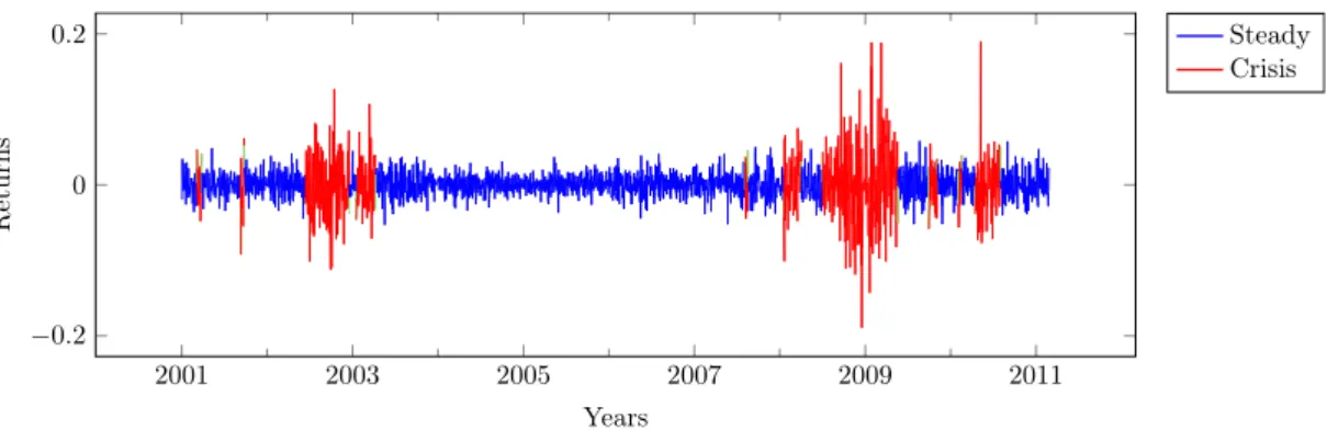
Once the model parameters are determined, we solve the recognition problem by the Viterbi algorithm [51], a dynamic programming algorithm for finding the most likely se-quence of hidden states corresponding to a sese-quence of observed events. In fact, the algorithm uses a global maximum a posteriori estimation of states to maximize the prob-abilities 𝛿𝑡p𝑖q of being in state 𝑖 at time 𝑡 knowing the partial sequence 𝑅1, . . . , 𝑅𝑡. Fig. 1

describes the state sequence built for the BNP stock. The crisis periods are in red and the steady periods are in blue.

This information of crisis periods is integrated in the estimation of return distribution as follows.

∙ We set 𝑡0 “ 1500 for getting enough data for the HMM estimation. For fixed 𝑡 ě 𝑡0,

the VaR at time 𝑡 is given by 𝑞𝐿_𝑎 as follows:

(a) Estimate the HMM parameters 𝑀1:𝑡´1 “ p𝜌1:𝑡´1, 𝑄1:𝑡´1, 𝜓1:𝑡´1q from the return sample p𝑅1, . . . , 𝑅𝑡´1q .

2001 2003 2005 2007 2009 2011 −0.2 0 0.2 Years Returns Steady Crisis

Figure 1: Classification and detection of crisis and steady periods for the BNP stock.

(b) Estimate the sequence of hidden states p𝑋1, . . . , 𝑋𝑡´1q .

(c) Estimate the power law parameters p𝐶𝑐, 𝛼𝑐q from the last 252 returns of crisis

periods of the sample p𝑅1, . . . , 𝑅𝑡´1q .

(d) Estimate power law parameters p𝐶𝑠, 𝛼𝑠q from the last 252 returns of steady

periods of the sample p𝑅1, . . . , 𝑅𝑡´1q .

(e) With

𝑝𝑡“ Pp𝑋𝑡“ 𝑐q “ Pp𝑋𝑡 “ 𝑐|𝑋𝑡´1 “ 𝑐qPp𝑋𝑡´1 “ 𝑐q ` Pp𝑋𝑡“ 𝑐|𝑋𝑡´1“ 𝑠qPp𝑋𝑡´1 “ 𝑠q

“ 𝑄0:𝑡´1p𝑐, 𝑐q 𝛿𝑡´10:𝑡´1p𝑐q ` 𝑄 0:𝑡´1

p𝑠, 𝑐q 𝛿0:𝑡´1𝑡´1 p𝑠q,

the quantile of the losses at level 𝑎 is obtained with

1 ´ 𝑎 “ 𝑝𝑡 𝐶𝑐 𝑥´𝛼𝑐 ` p1 ´ 𝑝𝑡q 𝐶𝑠 𝑥´𝛼𝑠.

This equation is then solved by using Newton-Raphson method. 3.4 Backtesting

The backtesting procedure consists in comparing the successive estimated VaR by moving window approach with the actual returns [11]. A violation occurs when the actual return 𝑅𝑡 is smaller than VaR𝑡p𝑎q estimated from the previous data. The violation ratio is

defined as the total number of violations, over the total number of one-period forecasts. When the VaR is estimated at p1 ´ 𝑎qth quantile, the expected violation ratio should be 𝑞 “ 1 ´ 𝑎. A higher violation ratio implies an under-estimation of the VaR. Conversely, a lower ratio implies an over-estimation of the VaR by the underlying model.

To construct the confidence interval (CI) for the violation ratio, the sum of 𝐼𝑡 of

one-period forecasts, where 𝐼𝑡 takes 1 if there is a violation otherwise 0, follows a binomial

distribution as we assume it is the sum of independent random variables. An exact CI at 100 ˆ p1 ´ 𝜃q% is given by « 1 1 ` 𝑛´𝑘`1_𝑘 𝐹2p𝑛´𝑘`1q,2𝑘p1 ´ 𝜃{2q , 𝑘`1 𝑛´𝑘𝐹2p𝑘`1q,2p𝑛´𝑘qp1 ´ 𝜃{2q 1 ` 𝑘`1<sub>𝑛´𝑘</sub>𝐹2p𝑘`1q,2p𝑛´𝑘qp1 ´ 𝜃{2q ff ,

where 𝑘 is the success number, 𝑛 the sample size, and 𝐹𝜈1,𝜈2p𝑝q the inverse of the quantile

at level 𝑝 P r0, 1s of the Fisher 𝐹 -distribution with degree of freedoms 𝜈1 and 𝜈2 [8, 9].

In order to test our assumption of independence of the 𝐼𝑡, we use the unconditional

CC tests jointly independence and correct coverage. It combines the UC test and a test of independence. The likelihood ratio (LR) of the CC test is given by [12]:

𝐿𝑅𝑐𝑐 “ 𝐿𝑅𝑢𝑐` 𝐿𝑅𝑖𝑛𝑑

“ ´2 ln“𝑞𝑁p1 ´ 𝑞q𝑇 ´𝑁‰ ` 2 ln rp1 ´ 𝜋01q𝑛00𝜋01𝑛01p1 ´ 𝜋11q𝑛10𝜋11𝑛11s „ 𝜒 2

p2q (11)

where 𝑇 is the number of observations, 𝑁 is the number of violations, 𝑞 “ 1 ´ 𝑎 where 𝑎 is the confidence level, 𝑛𝑖𝑗 is the number of observations with value 𝑖 followed by 𝑗,

and 𝜋𝑖𝑗 “ Pp𝐼𝑡 “ 𝑗|𝐼𝑡´1 “ 𝑖q is the probability value. The first part of (11) is the

LR of the unconditional coverage test p𝐿𝑅𝑢𝑐q, and the second part of (11) is the LR of

the independence test p𝐿𝑅𝑖𝑛𝑑q. In the case of 𝑛11 “ 0, the 𝐿𝑅𝑐𝑐 will be limited to the

first-order Markov likelihood as given in [13]: 𝐿𝑅𝑐𝑐“ ´2 ln“𝑞𝑁p1 ´ 𝑞q𝑇 ´𝑁

‰

` 2 ln rp1 ´ 𝜋01q𝑛00𝜋01𝑛01s „ 𝜒 2

p2q. (12)

In our numerical study (section 4), we estimate a VaR at 1% confidence level, as in Basel II requirements [50]. VaR forecasting performances of our models are compared by the violation ratio, the exact confidence interval test and the UC and CC Christoffersen tests.

4

Discussion: Empirical results and backtesting analysis

4.1 The dataset: stocks from Euronext Paris

The financial instruments considered in the experiments are stocks exchanged on NYSE Euronext Paris. The market data are provided by eSignal (Interactive Data), and, in the following, the stocks are identified by their eSignal symbol. Out of all the stocks listed on the Euronext Paris exchange in February 2011 (more than 600), we selected those having quotations throughout all the period ranging from January 2001 till February 2011 (more than 11 years). This leads us with a subset of 56 stocks including some of the most liquid stocks making up the CAC40 index. The list of these assets can be found in Table 1. In the following experiments, the time series considered are the returns of the end-of-day closing prices of the selected stocks and the parameters of the returns distributions are estimated on a sample as explained in section 3.3. The choice of a window length set to one year, in models I and II, is a trade-off between the need to have enough data to make good calibration and to include recent crises and the increased risk of departure from the stationarity hypothesis with larger datasets. Regarding the stationarity, it is difficult to draw a clear cut conclusion from Dickey-Fuller and Kwiatkowski–Phillips–Schmidt–Shin tests on unit root and stationarity tests [20, 34]. In our experiments, we are not able to identify other sample sizes that would consistently outperform one year with regard to the VaR backtesting or stationarity measures.

4.2 Discussion

In this section, the relative forecasting performances of the regime switching and bench-marked models are illustrated. We apply the methods of estimation of the Value-at-Risk and of backtesting described in Section 3 on the dataset described above. We plot for all stocks their prices, historical volatility computed from one-year data over a moving window, and VaR computed under our four models. Our comparisons are based on a backtesting for a single level of confidence one level of confidence 1% of the VaR. The performance of each model is given by an average of its results for the selected stocks.

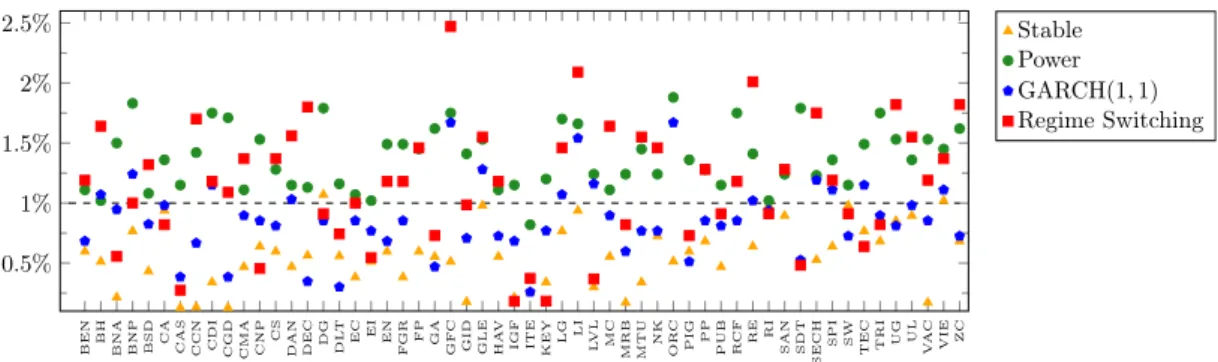
Fig. 2 gives the violation ratios for the four models on the 56 selected stocks. Clearly the stable model over-estimates the VaR and the power law model under-estimates the

BEN BH BNA BNP BSD CA CAS CCN CDI CGD CMA CNP CS DAN DEC DG DL T EC EI EN F GR FP GA GF C GID GLE HA V

IGF ITE _KEY LG LI LVL MC MRB MTU NK OR

C

PIG PP PUB RCF RE RI SAN SDT

SECH

SPI SW _TEC TRI UG UL VA

C VIE ZC 0.5% 1% 1.5% 2% 2.5% _Stable Power GARCH(1, 1) Regime Switching

Figure 2: Violation ratios of 56 Euronext Paris stocks under the four estimation models.

VaR. GARCH and regime switching models results fluctuate around the target value 1%. In term of average of violation ratios, the regime switching model is the closest to 1% with 1.12%, followed by 0.86% for the GARCH model, then the power law model with 1.37% and the stable model with 0.55%. The number of stocks for which the backtest results in r0.90%, 1.10%s is 8 for the regime switching, 8 for the GARCH, 5 for the power law and 7 for the stable model.

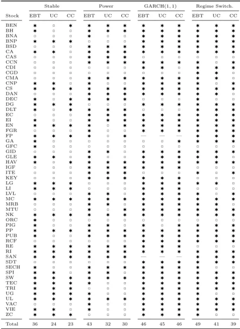
Due to the small amount of data available for the backtest, the confidence intervals (CI) are quite large. The average size of the CI is 0.39% for the stable distribution, 0.60% for the power law distribution, 0.98% for the GARCH model and 0.80% for the regime switching model. So it is not possible to give affirmative conclusions for a single stock, but the backtest results over the 56 stocks in Table 1 indicate that the regime switching model gives the best results in terms of backtest. With the regime switching model, 49 out of the 56 exact-CI contain the target value 1%. It is the case for only 46, 43 and 36 out of the 56 with the GARCH, power law and stable models respectively. The unconditional and conditional coverage tests give better results for the GARCH followed by the regime switching model. The results of UC and CC tests are given in Table. 1.

We can interpret this result as follows: the tail distribution in the stable law is too fat (since its tail index 𝛼 is always smaller than 2). This is confirmed by the fact that the estimated tail index for stable distribution is close to 2 for all stocks in our dataset. On the other hand, the tail of the power law distribution estimated on the full dataset is not fat enough to describe Euronext Paris market during crisis periods. The regime switching model computes a combination of tail power law for crisis and steady periods which produces a fatter tail distribution.

Fig. 3 shows the quantile estimations on our typical example BNP Paribas stock. As stable and power law models do not take into consideration the regime switching, they suffer from a delay in the estimation of the quantile. The beginning of periods of small (resp. large) fluctuations is characterized by an over-estimation (resp. under-estimation) of the VaR. However, by detecting the volatility clustering, the GARCH model takes into consideration the regime switching and overcomes this drawback of under-estimation and over-estimation. Our new HMM approach aims to give a simpler model that combines the advantage of power law and GARCH models. We consider crisis and steady periods and we combine their tail power law distributions. This permits at the beginning of large fluctuations (crisis periods) to reduce the VaR threshold due to the additional term computed from previous crisis periods. Similarly, at the beginning of small fluctuations (steady periods), it permits to raise the VaR threshold by adding a term computed from previous steady periods. The consideration of two states in our model allows to reduce the delay of regime switching detection in the quantile estimation while keeping the model

Stable Power GARCHp1, 1q Regime Switch.

Stock EBT UC CC EBT UC CC EBT UC CC EBT UC CC

BEN › ˝ › › › › › › › › › › BH › ˝ ˝ › › › › › › › › › BNA ˝ ˝ ˝ › ˝ ˝ › › › › › › BNP › › › ˝ ˝ ˝ › › › › › › BSD ˝ ˝ ˝ › › › › › › › › › CA › › ˝ › › › › › › › › › CAS ˝ ˝ ˝ › › › ˝ ˝ ˝ ˝ ˝ ˝ CCN ˝ ˝ ˝ › › › › › › › ˝ › CDI ˝ ˝ ˝ ˝ ˝ ˝ › › ˝ › › › CGD ˝ ˝ ˝ ˝ ˝ ˝ ˝ ˝ ˝ › › ˝ CMA ˝ ˝ ˝ › › › › › › › › ˝ CNP › › ˝ › ˝ ˝ › › › › ˝ › CS › › › › › › › › › › › › DAN ˝ ˝ ˝ › › › › › › › › ˝ DEC › ˝ › › › › ˝ ˝ ˝ › ˝ ˝ DG › › › ˝ ˝ ˝ › › › › › › DLT › ˝ › › › › ˝ ˝ ˝ › › › EC ˝ ˝ ˝ › › › › › › › › › EI › ˝ ˝ › › › › › › › › › EN › › › › ˝ › › › › › › › FGR ˝ ˝ ˝ › ˝ ˝ › › › › › › FP › › › › ˝ › — — — › › › GA › ˝ ˝ ˝ ˝ ˝ ˝ ˝ › › › › GFC › ˝ ˝ ˝ ˝ ˝ ˝ ˝ ˝ ˝ ˝ ˝ GID ˝ ˝ ˝ › › ˝ › › › › › › GLE › › ˝ › ˝ ˝ › › › › › ˝ HAV › ˝ › › › › › › › › › › IGF ˝ ˝ ˝ › › › › › › ˝ ˝ ˝ ITE ˝ ˝ ˝ › › › ˝ ˝ ˝ › ˝ › KEY ˝ ˝ ˝ › › › › › › ˝ ˝ ˝ LG › › › ˝ ˝ ˝ › › › › › ˝ LI › › › ˝ ˝ ˝ › › › ˝ ˝ ˝ LVL ˝ ˝ ˝ › › ˝ › › › › ˝ › MC › › › › › › › › › › › › MRB ˝ ˝ ˝ › › ˝ › › › › › ˝ MTU ˝ ˝ ˝ › ˝ › › › › › › › NK › › › › › › › › › › › › ORC › ˝ ˝ ˝ ˝ ˝ ˝ ˝ ˝ ˝ ˝ ˝ PIG › ˝ ˝ › › ˝ › ˝ › › › › PP › › › › › › › › › › › › PUB › ˝ ˝ › › › › › › › › › RCF ˝ ˝ ˝ ˝ ˝ ˝ › › › › › › RE › › › › › › › › › ˝ ˝ ˝ RI › › › › › › › › › › › › SAN › › › › › › — — — › › › SDT ˝ ˝ ˝ ˝ ˝ ˝ › › › › › › SECH › ˝ ˝ › › › › › › › ˝ ˝ SPI › › ˝ › › ˝ › › › › › › SW › › › › › › › › › › › › TEC › › › › ˝ ˝ › › › › › › TRI › › › ˝ ˝ ˝ › › › › › › UG › › › › ˝ ˝ › › › › ˝ ˝ UL › › › › › › › › › › › › VAC ˝ ˝ ˝ › ˝ ˝ › › › › › › VIE › › ˝ › ˝ ˝ › › › › › › ZC › › › ˝ ˝ ˝ › › › › ˝ ˝ Total 36 24 23 43 32 30 46 45 46 49 41 39

›Fail to reject, ˝Rejection, — Not converging

Table 1: Exact CI backtesting (EBT) and unconditional (UC) and conditional coverage (UC) tests over 56 Euronext Paris stocks.

simple.

5

Conclusions and perspectives

Value-at-Risk (VaR) and conditional volatility models have become common tools for fi-nancial forecasting. However, conditional volatility models cannot capture extreme move-ments, as these models are based on past volatility rather than the extreme observations. On the other hand, extreme value theory models can capture extreme movements and forecasting performance of these models are better than that of conventional volatility models such as GARCH. In this paper, hidden Markov models and EVT are combined to construct a variant of power laws model that forecasts the extreme observations taking into consideration both the data clustering and the regime switching.

The main contribution of this paper is to propose a combined EVT model and compare the predictive performance of this model with conventional models. This hybrid model

2001 2003 2005 2007 2009 2011 −0.3 −0.2 −0.1 0 0.1 0.2 Years Returns and 1% V aR threshold for the BNP sto ck Returns_Stable Power GARCH(1, 1) Regime Switching

Figure 3: Comparison of 1% VaR models for the BNP stock.

is tested on real data of 56 stocks exchanged on NYSE Euronext Paris. The relative performance of regime switching model is benchmarked against stable, power laws and GARCH-𝑡 models. Our regime switching model gives an average violation ratio on 56 stocks closer to 1% than the other models, and the model is statistically significant for all Christoffersen [12] tail-loss tests for most of the stocks. The regime switching model has the advantage of a simple power law model in the threshold estimation. In addition, it reduces the violation clustering observed in stable and power law models by taking into account the crisis and steady periods. However, it shows a fluctuation over and under the target value 1% in the backtest results characterizing almost all conditional models.

Our results suggest further study by classifying data with a long-memory model of hidden states to have more stability in the VaR forecasting. Co-movements and corre-lations between stocks in terms of crisis periods can be studied to identify global crisis periods or classes of stocks that have the same behavior. Such clustering would permit to refine the model for each class of stocks and further increase the performance of VaR forecasting.

Acknowledgment

This work was partially supported by a collaboration between the SME Alphability and Inria.

References

[1] C. Alexander and E. Sheedy. “Developing a stress testing framework based on mar-ket risk models”. In: Journal of Banking & Finance 32.10 (2008), pp. 2220–2236. [2] A. Ang and G. Bekaert. “Regime Switches in Interest Rates”. English. In: Journal

of Business Economic Statistics 20.2 (2002), pp. 163–182. issn: 07350015.

[3] L. E. Baum and T. Petrie. “Statistical inference for probabilistic functions of finite state Markov chains”. In: Ann. Math. Statist. 37 (1966), pp. 1554–1563. issn: 0003-4851.

[4] L. E. Baum, T. Petrie, G. Soules, and N. Weiss. “A maximization technique occur-ring in the statistical analysis of probabilistic functions of Markov chains”. In: Ann. Math. Statist. 41 (1970), pp. 164–171. issn: 0003-4851.

[5] J. Beirlant, Y. Goegebeur, J. Teugels, and J. Segers. Statistics of extremes. Wiley Series in Probability and Statistics. Theory and applications, With contributions from Daniel De Waal and Chris Ferro. John Wiley & Sons Ltd., 2004.

[6] J. Berkowitz and J. O’Brien. “How Accurate Are Value-at-Risk Models at Commer-cial Banks?” In: The journal of finance 57.3 (2002), pp. 1093–1111.

[7] M. Billio and L. Pelizzon. “Value-at-Risk: a multivariate switching regime approach”. In: Journal of Empirical Finance 7.5 (2000), pp. 531 –554. issn: 0927-5398.

[8] C. R. Blyth. “Approximate binomial confidence limits”. In: J. Amer. Statist. Assoc. 81.395 (1986), pp. 843–855.

[9] C. R. Blyth. “Correction: “Approximate binomial confidence limits” [J. Amer. Statist. Assoc. 81 (1986), no. 395, 843–855]”. In: J. Amer. Statist. Assoc. 84.406 (1989), p. 636.

[10] S. A. Broda, M. Haas, J. Krause, M. S. Paolella, and S. C. Steude. “Stable mixture GARCH models”. In: Journal of Econometrics 17 (2013), pp. 292–316.

[11] S. D. Campbell. A review of backtesting and backtesting procedures. Tech. rep. 2007, pp. 1–17.

[12] P. F. Christoffersen. “Evaluating interval forecasts”. In: Internat. Econom. Rev. 39.4 (1998). Symposium on Forecasting and Empirical Methods in Macroeconomics and Finance, pp. 841–862. issn: 0020-6598.

[13] P. Christoffersen and D. Pelletier. “Backtesting Value-at-Risk: A Duration-Based Approach”. In: Journal of Financial Econometrics 2.1 (2004), pp. 84–108. eprint: http://jfec.oxfordjournals.org/content/2/1/84.full.pdf+html.

[14] A. Cifter. “Value-at-risk estimation with wavelet-based extreme value theory: Evi-dence from emerging markets”. In: Physica A: Statistical Mechanics and its Appli-cations 390.12 (2011), pp. 2356 –2367. issn: 0378-4371.

[15] P. K. Clark. “A subordinated stochastic process model with finite variance for specu-lative prices”. In: Econometrica: Journal of the Econometric Society (1973), pp. 135– 155.

[16] R. Cont. “Empirical properties of asset returns: stylized facts and statistical issues”. In: Quantitative Finance 1 (2001), pp. 223–236.

[17] R. Cont and P. Tankov. Financial modelling with jump processes. Chapman & Hall/CRC Financial Mathematics Series. Chapman & Hall/CRC, Boca Raton, FL, 2004.

[18] J. D. Curto, J. C. Pinto, and G. N. Tavares. “Modeling stock markets’ volatility using GARCH models with Normal, Student’s t and stable Paretian distributions”. In: Statistical Papers 50.2 (July 2007), pp. 311–321.

[19] J. Danielsson and Y. Morimoto. “Forecasting Extreme Financial Risk: A Critical Analysis of Practical Methods for the Japanese Market”. In: Monetary and Economic Studies 18.2 (2000).

[20] D. A. Dickey and W. A. Fuller. “Distribution of the estimators for autoregressive time series with a unit root”. In: J. Amer. Statist. Assoc. 74.366, part 1 (1979), pp. 427–431.

[21] F. X. Diebold, T. Schuermann, and J. D. Stroughair. “Pitfalls and Opportunities in the Use of Extreme Value Theory in Risk Management”. In: The Journal of Risk Finance 1.2 (2000), pp. 30–35.

[22] T. Doganoglu, C. Hartz, and S. Mittnik. “Portfolio optimization when risk factors are conditionally varying and heavy tailed”. In: Computational Economics 29.3-4 (Jan. 2007), pp. 333–354.

[23] W. H. DuMouchel. “Estimating the Stable Index 𝛼 in Order to Measure Tail Thick-ness: A Critique”. In: the Annals of Statistics 11.4 (1983), pp. 1019–1031.

[24] E. F. Fama. “Risk, return, and equilibrium”. In: The Journal of Political Economy 791.1 (1971), pp. 30–55.

[25] H. Fofack and J. P Nolan. “Tail behavior, modes and other characteristics of stable distributions”. In: Extremes 2.1 (1999), pp. 39–58.

[26] R. Gençay and F. Selçuk. “Extreme value theory and Value-at-Risk: Relative per-formance in emerging markets”. In: International Journal of Forecasting 20.2 (Apr. 2004), pp. 287–303.

[27] R. Gençay, F. Selçuk, and A. Ulugülyağci. “High volatility, thick tails and extreme value theory in value-at-risk estimation”. In: Insurance: Mathematics and Economics 33.2 (2003). Papers presented at the 6th IME Conference, Lisbon, 15-17 July 2002, pp. 337 –356. issn: 0167-6687.

[28] M. Gilli and E. Këllezi. “An Application of Extreme Value Theory for Measuring Financial Risk”. In: Computational Economics 27.2-3 (2006), pp. 207–228.

[29] A. Gulisashvili. Analytically tractable stochastic stock price models. Springer Fi-nance. Heidelberg: Springer, 2012.

[30] J. D. Hamilton. “Specification testing in Markov-switching time-series models”. In: Journal of Econometrics 70.1 (1996), pp. 127 –157. issn: 0304-4076.

[31] D. W. Jansen and C. G. de Vries. “On the frequency of large stock returns: Putting booms and busts into perspective”. In: The review of economics and statistics (1991), pp. 18–24.

[32] P. Jorion. Value at Risk: The New Benchmark for Managing Financial Risk. 3rd ed. McGraw-Hill, 2006.

[33] K. Kuester, S. Mittnik, and M. S. Paolella. “Value-at-risk prediction: A comparison of alternative strategies”. In: Journal of Financial Econometrics 4.1 (2006), pp. 53– 89.

[34] D. Kwiatkowski, P. Phillips, and P. Schmidt. “Testing the null hypothesis of sta-tionarity against the alternative of a unit root: How sure are we that economic time series have a unit root?” In: Journal of Econometrics 54 (1992), pp. 159–178. [35] F. Longin. “The Asymptotic Distribution of Extreme Stock Market Returns”. In:

The Journal of Business 69.3 (1996), pp. 383–408.

[36] M. Loretan and P. Philips. “Testing the covariance stationarity of heavy-tailed time series: An overview of the theory with applications to several financial datasets”. In: Journal of Empirical Finance 1.2 (1994), pp. 211–248.

[37] Y. Malevergne, V. Pisarenko, and D. Sornette. “On the power of generalized ex-treme value (GEV) and generalized Pareto distribution (GPD) estimators for em-pirical distributions of stock returns”. In: Applied Financial Economics 16.3 (2006), pp. 271–289.

[38] B. Mandelbrot. “The variation of certain speculative prices”. In: Journal of business XXXVI (1963), pp. 392–417.

[39] R. Marfè. “A generalized variance gamma process for financial applications”. In: Quantitative Finance 12.1 (Jan. 2012), pp. 75–87.

[40] J. H. McCulloch. “Measuring tail thickness to estimate the stable index 𝛼: a cri-tique”. In: J. Bus. Econom. Statist. 15.1 (1997), pp. 74–81.

[41] J. Mina and J. Y. Xiao. Return to RiskMetrics: The Evolution of a Standard. Tech. rep. RiskMetrics, 2001.

[42] Y. Nagahara. “Non-Gaussian distribution for stock returns and related stochas-tic differential equation”. In: Financial Engineering and the Japanese Markets 3.2 (1996), pp. 121–149.

[43] J. Nolan. Stable Distributions: Models for Heavy Tailed Data. Boston: Birkhauser, 2013.

[44] S. Rachev, ed. Handbook of Heavy Tailed Distributions in Finance, Volume 1. North-Holland, 2003.

[45] C. Scarrott and A. MacDonald. “A review of extreme value thresehold estima-tion and uncertainty quanticaestima-tion.” In: REVSTAT–Statistical Journal 10.1 (2012), pp. 33–60.

[46] H. Schaller and S. V. Norden. “Regime switching in stock market returns”. In: Applied Financial Economics 7.2 (1997), pp. 177–191. eprint: http : / / dx . doi . org/10.1080/096031097333745.

[47] R. Serfling. “Quantile functions for multivariate analysis: approaches and applica-tions”. In: Statistica Neerlandica 56.2 (2002), pp. 214–232.

[48] W. T. Shaw and M. Schofield. “A model of returns for the post-credit-crunch reality: hybrid Brownian motion with price feedback”. In: Quantitative Finance (Jan. 2012), pp. 1–24.

[49] A. Singh, D. Allen, and P. Robert. “Extreme Market Risk and Extreme Value The-ory”. In: Mathematics and computers in simulation 94 (2013), pp. 310 –328.

[50] Supervision, Basel Committee on Banking, ed. International Convergence of Capital Measurement and Capital Standards – A Revised Framework. Bank of International Settlements, June 2004.

[51] A. Viterbi. “Error bounds for convolutional codes and an asymptotically optimum decoding algorithm”. In: Information Theory, IEEE Transactions on 13.2 (1967), pp. 260–269. issn: 0018-9448.

[52] I. Weissman. “Estimation of parameters and large quantiles based on the 𝑘 largest observations”. In: J. Amer. Statist. Assoc. 73.364 (1978), pp. 812–815.

[53] R. Weron. “Levy-stable distributions revisited: tail index ą 2 does not exclude the Levy-stable regime”. In: International Journal of Modern Physics C. 12.2 (2001), pp. 209–223.