A general non-stationarity measure : Application to biomedical image and signal processing

(1)

HAL Id: tel-01127038

https://tel.archives-ouvertes.fr/tel-01127038

Submitted on 6 Mar 2015

HAL is a multi-disciplinary open access archive for the deposit and dissemination of sci-entific research documents, whether they are pub-lished or not. The documents may come from

L’archive ouverte pluridisciplinaire HAL, est destinée au dépôt et à la diffusion de documents scientifiques de niveau recherche, publiés ou non, émanant des établissements d’enseignement et de

Yanli Xu

To cite this version:

Yanli Xu. A general non-stationarity measure : Application to biomedical image and signal processing. Imaging. INSA de Lyon, 2013. English. �NNT : 2013ISAL0090�. �tel-01127038�

(2)

THÈSE

présentée devant

L’Institut National des Sciences Appliquées de Lyon

pour obtenir

LE GRADE DE DOCTEUR

ÉCOLE DOCTORALE: ÉLECTRONIQUE, ÉLECTROTECHNIQUE, AUTOMATIQUE FORMATION DOCTORALE : SCIENCES DE L’INFORMATION, DES DISPOSITIFS ET

DES SYSTÈMES par

ZHANG Yanli

Une mesure de non-stationnarité générale: application en traitement

d'images et de signaux biomédicaux

Soutenue le 04 Octobre 2013 Jury :

Jean-Marc CHASSERY Directeur de Recherche CNRS Rapporteur

Isabelle BLOCH Professeur ENST Rapporteur

Isabelle E. MAGNIN Directeur de recherche INSERM Directeur de thèse

Yue-Min ZHU Directeur de recherche CNRS Codirecteur de thèse

Jin LI Professeur d’HEU Examinateur

Ping LI Professeur, Radiologue Hospitalier de

HMU

Examinateur

(3)

CHIMIE

CHIMIE DE LYON

http://www.edchimie-lyon.fr

Insa : R. GOURDON

M. Jean Marc LANCELIN Université de Lyon – Collège Doctoral Bât ESCPE

43 bd du 11 novembre 1918 69622 VILLEURBANNE Cedex Tél : 04.72.43 13 95

[email protected]

E.E.A. ELECTRONIQUE, ELECTROTECHNIQUE, AUTOMATIQUE http://edeea.ec-lyon.fr

Secrétariat : M.C. HAVGOUDOUKIAN [email protected]

M. Gérard SCORLETTI Ecole Centrale de Lyon 36 avenue Guy de Collongue 69134 ECULLY

Tél : 04.72.18 60 97 Fax : 04 78 43 37 17

[email protected]

E2M2 EVOLUTION, ECOSYSTEME, MICROBIOLOGIE, MODELISATION http://e2m2.universite-lyon.fr

Insa : H. CHARLES

Mme Gudrun BORNETTE CNRS UMR 5023 LEHNA

Université Claude Bernard Lyon 1 Bât Forel

43 bd du 11 novembre 1918 69622 VILLEURBANNE Cédex Tél : 04.72.43.12.94

[email protected]

EDISS INTERDISCIPLINAIRE SCIENCES- SANTE http://ww2.ibcp.fr/ediss

Sec : Safia AIT CHALAL Insa : M. LAGARDE

M. Didier REVEL Hôpital Louis Pradel Bâtiment Central 28 Avenue Doyen Lépine 69677 BRON

Tél : 04.72.68 49 09 Fax : 04 72 35 49 16

[email protected]

INFOMATHS INFORMATIQUE ET MATHEMATIQUES

http://infomaths.univ-lyon1.fr

M. Johannes KELLENDONK Université Claude Bernard Lyon 1 INFOMATHS Bâtiment Braconnier 43 bd du 11 novembre 1918 69622 VILLEURBANNE Cedex Tél : 04.72. 44.82.94 Fax 04 72 43 16 87 [email protected] Matériaux MATERIAUX DE LYON Secrétariat : M. LABOUNE PM : 71.70 –Fax : 87.12 Bat. Saint Exupéry

[email protected]

M. Jean-Yves BUFFIERE INSA de Lyon

MATEIS

Bâtiment Saint Exupéry 7 avenue Jean Capelle 69621 VILLEURBANNE Cédex

Tél : 04.72.43 83 18 Fax 04 72 43 85 28

[email protected]

MEGA MECANIQUE, ENERGETIQUE, GENIE CIVIL, ACOUSTIQUE Secrétariat : M. LABOUNE

PM : 71.70 –Fax : 87.12 Bat. Saint Exupéry

[email protected]

M. Philippe BOISSE INSA de Lyon Laboratoire LAMCOS Bâtiment Jacquard 25 bis avenue Jean Capelle 69621 VILLEURBANNE Cedex

Tél :04.72.43.71.70 Fax : 04 72 43 72 37

[email protected]

ScSo ScSo*

M. OBADIA Lionel

Sec : Viviane POLSINELLI Insa : J.Y. TOUSSAINT

M. OBADIA Lionel Université Lyon 2 86 rue Pasteur 69365 LYON Cedex 07 Tél : 04.78.69.72.76 Fax : 04.37.28.04.48 [email protected]

(4)

A General Non-Stationarity Measure: Application to

Biomedical Image and Signal Processing

Abstract

The intensity variation is often used in signal or image processing algorithms after being quantified by a measurement method. The method for measuring and quantifying the intensity variation is called a « change measure », which is commonly used in methods for signal change detection, image edge detection, edge-based segmentation models, feature-preserving smoothing, etc. In these methods, the « change measure » plays such an important role that their performances are greatly affected by the result of the measurement of changes.

The existing « change measures » may provide inaccurate information on changes, while processing biomedical images or signals, due to the high noise level or the strong randomness of the signals. This leads to various undesirable phenomena in the results of such methods. On the other hand, new medical imaging techniques bring out new data types and require new change measures. How to robustly measure changes in those tensor-valued data becomes a new problem in image and signal processing.

In this context, a « change measure », called the Non-Stationarity Measure (NSM), is improved and extended to become a general and robust « change measure » able to quantify changes existing in multidimensional data of different types, regarding different statistical parameters.

A NSM-based change detection method and a NSM-based edge detection method are proposed and respectively applied to detect changes in ECG and EEG signals, and to detect edges in the cardiac diffusion weighted (DW) images. Experimental results show that the NSM-based detection methods can provide more accurate positions of change points and edges and can effectively reduce false detections.

A NSM-based geometric active contour (NSM-GAC) model is proposed and applied to segment the ultrasound images of the carotid. Experimental results show that the NSM-GAC model provides better segmentation results with less iterations that comparative methods and can reduce false contours and leakages.

Last and more important, a new feature-preserving smoothing approach called « Nonstationarity adaptive filtering (NAF) » is proposed and applied to enhance human cardiac DW images. Experimental results show that the proposed method achieves a better compromise between the smoothness of the homogeneous regions and the preservation of desirable features such as boundaries, thus leading to homogeneously consistent tensor fields and consequently a more reconstruction of the coherent fibers.

Keywords: non-stationarity measure, change detection, edge detection, segmentation, adaptive filtering, diffusion tensor, magnetic resonance imaging, cardiac imaging

(5)

Une Mesure de Non-Stationnarité Générale: Application

en Traitement d'Images et de Signaux Biomédicaux

Résumé

La variation des intensités est souvent exploitée comme une propriété importante du signal ou de l’image par les algorithmes de traitement. La grandeur permettant de représenter et de quantifier cette variation d’intensité est appelée « mesure de changement », elle est couramment employée dans les méthodes de détection de ruptures d’un signal, en détection de contours d’une image, dans les modèles de segmentation basés sur les contours, et dans les méthodes de lissage d’images avec préservation de discontinuités.

En traitement des images et des signaux biomédicaux, les mesures de changement existantes fournissent des résultats peu précis lorsque le signal ou l’image présentent un fort niveau de bruit ou un fort caractère aléatoire, ce qui conduit à des artefacts indésirables dans le résultat des méthodes basées sur la mesure de changement. D’autre part, de nouvelles techniques d'imagerie médicale produisent de nouveaux types de données dites à valeurs multiples, qui nécessitent le développement de mesures de changement adaptées. Mesurer le changement dans des données de tenseur pose alors de nouveaux problèmes.

Dans ce contexte, une mesure de changement, appelée « mesure de non-stationnarité (NSM) », est améliorée et étendue pour permettre de mesurer la non-stationnarité de signaux multidimensionnels quelconques (scalaires, vectoriels, tensoriels) par rapport à un paramètre statistique, ce qui en fait ainsi une mesure générique et robuste.

Une méthode de détection de changements basée sur la NSM et une méthode de détection de contours basée sur la NSM sont respectivement proposées et appliquées aux signaux ECG et EEG, ainsi qu’a des images cardiaques pondérées en diffusion (DW). Les résultats expérimentaux montrent que les méthodes de détection basées sur la NSM permettent de fournir la position précise des points de changement et des contours des structures tout en réduisant efficacement les fausses détections.

Un modèle de contour actif géométrique basé sur la NSM (NSM-GAC) est proposé et appliqué pour segmenter des images échographiques de la carotide. Les résultats de segmentation montrent que le modèle NSM-GAC permet d’obtenir de meilleurs résultats comparativement aux outils existants avec moins d'itérations et un temps de calcul plus faible tout en réduisant les faux contours et les ponts.

Enfin, et plus important encore, une nouvelle approche de lissage préservant les caractéristiques locales, appelée filtrage adaptatif de non-stationnarité (NAF), est proposée et appliquée pour améliorer les images DW cardiaques. Les résultats expérimentaux montrent que la méthode proposée peut atteindre un meilleur compromis entre le lissage des régions homogènes et la préservation des caractéristiques désirées telles que les bords ou frontières, ce qui conduit à des champs de tenseurs plus homogènes et par conséquent à des fibres cardiaques reconstruites plus cohérentes.

Mots Clés: mesure de Non-stationnarité, détection de changement, détection de contours, segmentation, filtrage adaptatif, tenseur de diffusion, imagerie par résonance magnétique, imagerie cardiaque

(6)

Acknowledgement

I owe my sincere gratitude to all the people who have made this dissertation possible and my graduate school experience a cherishable one.

I would like to express my deepest gratitude to my supervisors Madam Isabelle Magnin, Mr. Wan-Yu Liu and Mr. Yue-Min Zhu, not only for the guidance and supervision throughout the course of this work but also for their understanding, encouragement and kindness during these years. This thesis would not appear in its present form without their kind assistance and valuable suggestions. They have been phenomenal role models and special friends to me.

I would like to acknowledge the members of my thesis committee, especially the rapporteurs, Mr. Jean-Marc Chassery and Madam Isabelle Bloch. Thank you for agreeing to be my thesis rapporteurs and giving me valuable advice on my thesis. I would like to thank Professor Jin Li, president of the jury, for her valuable advice and kindness. I also thank Professor Ping Li for agreeing to be the member of my thesis committee.

I have had the priviledge of working in two outstanding labs: the Centre de Recherche en Acquisition et Traitement de l’Image pour la Santé (Creatis) and the HIT-INSA Sino-French Research Center for biomedical imaging. I would like to thank all members of both labs, past and present, for their support. In particular, I would like to thank Dr. Lihui Wang, Dr. Feng Yang and Shengfu Li for all their generous help. I also thank Dr. Pierre Croisille, Dr. Xin Song, Dr. Stanislas Rappachi, Dr. Carole Frindel and other researchers from Creatis for sharing their experiences and helpful discussions. And from the HIT-INSA Sino-French Research Center for biomedical imaging, I would also like to thank Jian-Ping Huang, Bin Gao, Kaixiang Zhang, Liu He, Dr. Li-Jun Bao, Qi Wu, Wen-Hui Liu, Shan Hu, Xiaoming Sun, and Jian-Wei Ma for their help.

I am profoundly grateful to my husband Jin-Zhe Xu and our parents for their unwavering love, understanding, and moral support during these years.

(7)

Content of Figures

Fig. 1.1 Signal segments X , Y and Z involved in the measurement of the change at time t0.... ... 8

Fig. 1.2 Main contents and the organization of the thesis ... 21

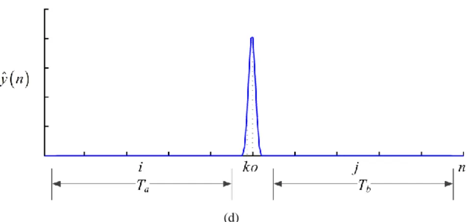
Fig. 2.1 Relationship among the signal x(n), the moving statistical parameter ˆ( ) n , the moving feature space R2W+1, and the NSM y nˆ( ). (a) Signal x(n) with a transition at time o. (b) Moving statistical parameter ˆ( ) n . (c) Multidimensional moving feature space R2W+1. (d) NSM y nˆ( ) of the signal x(n)... ... 27

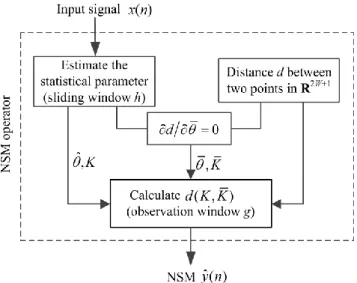
Fig. 2.2 Diagram for the calculation of the NSM y nˆ( ).... ... 30

Fig. 2.3 Block diagram of the 2nd-order NSM operator regarding the 1st-order moment of the signal x(n) ... 31

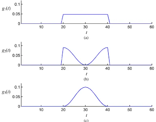
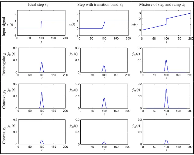
Fig. 2.4 Three typical input signals. (a) Ideal step s . (b) Step with transition band 1 s . (c) Mixture of step and 2 ramp s ... ... 33 3 Fig 2.5 Three typical observation window functions g. (a) Rectangular g1. (b) Concave g2. (c) Convex g3...34

(10)

Fig. 2.6 Output peaks of NSM operators regarding to typical input signals and window functions.... ... 36 Fig. 2.7 Trend graph of H_{2 j} for the step with transition band s2 ... 36

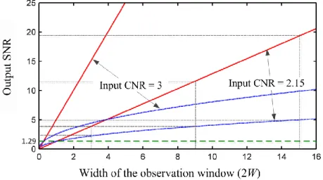
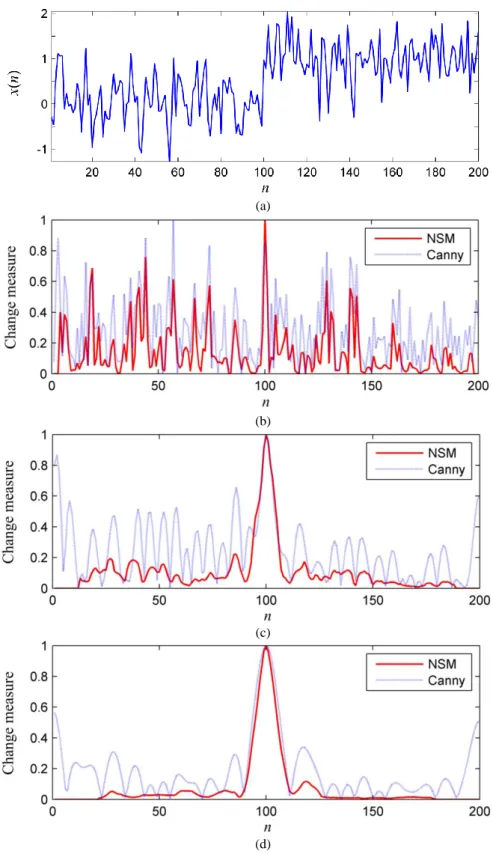
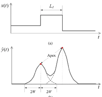
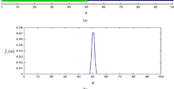
Fig. 2.8 Response peaks of the NSM operators to noisy input signals. ... 37 Fig. 2.9 Curves of output SNR of the NSM and the Canny operators. Red solid line: the NSM operator. Blue dashed line: the Canny operator. ... 41 Fig. 2.10 Comparison between the responses of the NSM operator and the Canny operator to the input signal with CNR2.15. (a) Unit step signal with a discontinuity at t100 corrupted by a white centered Gaussian noise. (b) 2W3 ,  0.96 . (c) 2W9,  2.88 . (d) 2W15 ,  4.80. All the outputs are normalized by their own maxima since the contrast is the thing that really matters in this comparison... .... 42 Fig. 2.11 Determination of the maximum of the window width. (a) A detail of width L . (b) The NSM of the _d detail... ... 44 Fig. 3.1 Block diagram of the 2nd-order NSM regarding the rth-order moment of the signal x(n)... ... 49 Fig.3.2 NSMs of a noisy signal containing a step in its 2nd-order moment. (a) x(n): noisy signal with a step at

501

n in its 2nd-order moment. (b) y n : NSM regarding the 1ˆ ( )1

st

-order moment (W20). (c) y n : ˆ ( )2

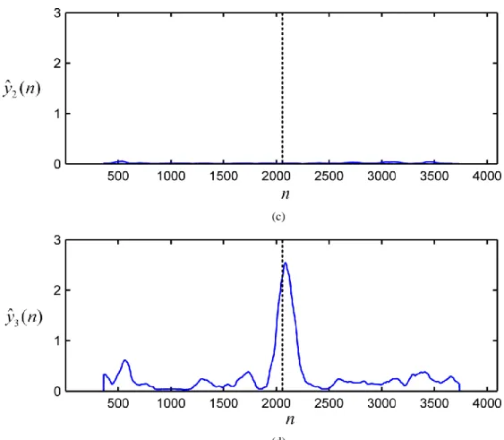
NSM regarding the 2nd-order moment (W20)... ... 50 Fig. 3.3 NSMs of a random signal containing a change in its 3rd-order moment. (a) x(n): random signal with a change at n2049 in its 3rd-order moment. (b) y n : NSM regarding the 1ˆ ( )₁ st-order moment (W120). (c)

2

ˆ ( )

y n : NSM regarding the 2nd-order moment (W120). (d) y n : NSM regarding the 3ˆ ( )3

rd

-order moment (W120)... ... 53 Fig. 3.4 NSMs of a noisy signal containing a change in its 4th-order moment. (a) x n( ): noisy signal with a change

at n2001 in its 4th_{-order moment. (b)}

1

ˆ ( )

y n : NSM regarding the 1st-order moment (W100). (c) y n : ˆ ( )₂

NSM regarding the 2nd-order moment (W100). (d) y n : NSM regarding the 3ˆ ( )₃ rd-order moment (W100). (e) y n : NSM regarding the 4ˆ ( )₄ th-order moment (W100)... ... 56 Fig.3.5 Determination of the state point in the moving feature space for 1-D to N-D data... ... 57 Fig.3.6 1-D vector-valued signal and its NSM. (a) 1-D vector-valued signal. (b) y n : NSM of the 1-D vector-ˆ ( )1

valued signal... ... 59 Fig.3.7 2-D vector field and its NSM map. (a) 2-D vector field composed of v1, v2, v3 successively. (b) relative

angular orientations of the three vector field. (c) NSM map of the 2-D vector field regarding its 1st_-order

moment. (d) Horizontal profile of (c)... ... 60 Fig. 3.8 1-D tensor signal and its NSM. (a) 1-D tensor signal. (b) y n : NSM of the 1-D tensor signal with the ˆ ( )1

detection of a 1st order moment change... ... 62 Fig. 3.9 2-D tensor field and its NSM map. (a) 2-D tensor fields composed of successively T1, T2, and T3. (b)

Ellipsoid T1, T2, and T3 (from left to right). (c) NSM map of the 2-D tensor field showing two changes of

their 1st order moment. (d) Horizontal profile of (c). ... 63 Fig. 4.1 Change detection of noisy synthetic signals. (a) Noisy synthetic signal x n with three steps in its 1₁( ) st

-order moment. (b) Noisy synthetic signal x n with three steps in its 2₂( ) nd-order moment. (c) y n : NSM of ˆ ( )₁ the noisy synthetic signal x n . (d) 1( ) y nˆ ( )2 : NSM of the noisy synthetic signal x n .... ... 68 2( )

Fig. 4.2 Heart rate signal of a new born baby and its change measurement curves. (a) The heart rate signal. (b) to (d) Change measurement curves obtained using the △BIC, the Pearson divergence, and the NSM y n , ˆ ( )1

respectively. Signal is courtesy of Lavielle 1999. ... 70 Fig. 4.3 Change detection of the heart rate of a new born baby. Red arrows: the NSM-based method; green arrows:

the △BIC-based method; magenta arrows: the Pearson divergence-based method; brown arrows: the DCPC ... 70 Fig. 4.4 EEG signal and its change measurement curves. (a) EEG signal. (b) to (d) Change measurement curves using the △BIC, the Pearson divergence and the NSM y nˆ ( )₂ respectively. Signal is courtesy of Lavielle 2005... ... 72

(11)

Fig. 4.5 Change detection of an EEG signal. Red arrows: the NSM-based method; green arrows: the △BIC-based method; magenta arrows: the Pearson divergence-based method; brown arrows: the DCPC... ... 73 Fig. 4.6 Nonmaxima suppression ... ... 74 Fig. 4.7 Noisy synthetic image and its change measurement maps obtained by the NLFS, the Canny filter, the FES method and the NSM operator... ... 75 Fig. 4.8 Edge detection of a noisy synthetic image. (a1) to (d1) Edges detected by the NLFS, the Canny filter, the FES method and the NSM-based method, respectively. (a2) to (d2) Upper left parts of (a1) to (d1)... ... 76 Fig. 4.9 Cardiac diffusion weighted image and its change measurement maps obtained by the NLFS, the Canny filter, the FES method and the NSM operator respectively. Images are courtesy of Pierre Croisille. ... 77 Fig. 4.10 Edge detection of a cardiac DW image. Edges detected by (a) the NLFS (Th0.25,Tl0.088), (b) the Canny filter (Th0.45,Tl0.158), (c) the FES method (Th0.4,Tl0.14) and (d) the NSM-based method (T_h0.22,T_l0.077), respectively.. ... 78 Fig. 5.1 Flow chart of the NSM-GAC model.... ... 84 Fig. 5.2 Segmentation of synthetic images with different noise levels... 86 Fig. 5.3 Segmentation of synthetic image corrupted by Gaussian noise. (a) Noisy synthetic image and the initial

contour. (b) to (d) Segmentation result of the DRLSE model, the C-V model and the NSM-GAC model... 88 Fig. 5.4 Simulated data. (a) backscatter cross section distribution. (b) Simulated carotid ultrasound image.... ... 90 Fig. 5.5 Segmentation of a simulated ultrasound image. (a) Simulated image and the initial contour. (b) to (d) Segmentation result of the DRLSE model, the C-V model and the NSM-GAC model... ... 91 Fig. 5.6 Segmentation of a real ultrasound image of a carotid. (a) Carotid image and the initial contour in red. (b) to (d) Segmentation results of the DRLSE model, the C-V model and the NSM-GAC model. Image is courtesy of Ping Li... ... 93 Fig. 6.1 Block diagram of the nonstationarity adaptive filtering (NAF) method... 98 Fig. 6.2 Determination of homogeneous 8-neighbors of the boundary point. ... ... 101 Fig. 6.3 Generation of a synthetic DW image similar to a slice of a human cardiac DTI volume. (a) Synthetic DW image. (b) Human cardiac DW image. Image is courtesy of Pierre Croisille.... ... 103 Fig. 6.4 Smoothing of synthetic human cardiac DW images in 6 diffusion gradient directions... ... 104 Fig. 6.5 Smoothing of synthetic cardiac DW images. (a) Noise-free DW image. (b) Noisy DW image. (c)

Smoothed by the ADF. (d) Smoothed by the NAF. (e)-(h) Profiles marked by the red dashed lines in (a)-(d)... ... 105 Fig. 6.6 Tensor fields in the Myocardium area before and after smoothing. (a)-(d) Tensor fields corresponding respectively to noise-free data, noisy, ADF smoothed and NAF smoothed cases. (e)-(h) Tensor fields in the red rectangles in (a)-(d)... ... 105 Fig. 6.7 Comparison of smoothing results obtained by the NAF and the ADF in terms of the MSSIM with different noise levels ranging from 5 to 25... ... 107 Fig. 6.8 Comparison of FA values of synthetic diffusion tensor data with different noise levels ranging from 5 to 25. (a) FA in the myocardium. (b) FA in the PF... ... 107 Fig. 6.9 Comparison of MD values of synthetic diffusion tensor data with different noise levels ranging from 5 to 25. (a) MD in the myocardium. (b) MD in the PF... ... 108 Fig. 6.10 Smoothing results of a real cardiac DW image. (a) Noisy DW image from an ex vivo human cardiac DTI datasets with 12 gradient directions. (b) Smoothed by the ADF. (c) Smoothed by the NAF. (d)-(f) Region circled by the red rectangles in (a)-(c). Images are courtesy of Pierre Croisille. ... ... 110 Fig. 6.11 Diffusion tensor fields corresponding to the region marked by the red rectangles in Fig. 6.10(a)-(c). (a) Noisy. (b) Smoothed by the ADF. (c) Smoothed by the NAF... ... 110 Fig. 6.12 Bundle of cardiac fibers lunching from a small patch of myocardium in the LV tracked from (a) the noisy data, (b) the smoothed data by the ADF, and (c) the smoothed data by the NAF. To indicate the locations of the fibers, they are overlapped with the original and the smoothed DW images, which are adjusted in color balance to highlight the fibers... ... 111

(12)

Introduction Générale

Les images et les signaux biomédicaux sont connus pour leur faible intensité, leur faible rapport signal sur bruit (SNR) et leurs fortes propriétés aléatoires. Améliorer la performance des méthodes de traitement pour ces données biomédicales est l'une des tâches importantes dans le domaine du traitement d'image et du signal.

La variation des intensités est souvent exploitée comme une propriété importante du signal ou de l’image par les algorithmes de traitement. La grandeur permettant de représenter et de quantifier cette variation d’intensité est appelée « mesure de changement ». Par exemple, l'amplitude du gradient est souvent utilisée comme une mesure de changement pour quantifier l’intensité des contours en traitement d'images. La « mesure de changement » est couramment employée dans les méthodes de détection des changements d’un signal, en détection de contours dans des images, dans les modèles de segmentation basés contours, et dans les méthodes de lissage d’images avec préservation de caractéristiques.

Dans toutes ces méthodes basées sur la «mesure de changement », la précision de cette mesure influence directement la performance de la méthode. En traitement d’images et de signaux biomédicaux, les mesures de changement existantes fournissent des résultats peu précis lorsque le signal ou l’image présente un fort niveau de bruit ou un fort caractère aléatoire, ce qui conduit à une dégradation des performances des méthodes basées ce type de mesure.

Dans ce contexte, l’objectif de notre travail de thèse est d'étudier une « mesure de changement » robuste et de l’utiliser pour améliorer la performance des méthodes de traitement du signal et de l’image, vis-à-vis du bruit et des artefacts indésirables souvent observés dans les méthodes existantes.

D’autre part, de nouvelles techniques d'imagerie médicale produisent de nouveaux types de données dites à valeurs multiples, qui nécessitent le développement des mesures de changement correspondantes. Par exemple, pour traiter les données de tenseur fournies par le DT-MRI, qui a apparu au milieu des années 1990, de nombreux travaux ont porté sur le traitement des champs de valeurs matricielles. Mesurer le changement dans ces données de tenseur pose alors de nouveaux problèmes en traitement d'images.

La mesure de non-stationnarité (NSM) est une mesure de changement robuste avec une bonne immunité au bruit. Elle peut refléter et quantifier les changements dans une image ou dans un signal en mesurant son degré de non-stationnarité. Dans ce travail, la méthode NSM est améliorée et étendue, et plusieurs approches de traitement d’image et de signal basées sur la NSM sont proposées et appliquées aux diverses images médicales ayant des niveaux de bruit élevés et aux signaux fortement aléatoires. En outre, la NSM étendue permet de mesurer les changements dans les données vectorielles et tensorielles, devenant ainsi une mesure générique et robuste pour des données de types différents et de dimensions quelconques. Les recherches effectuées sont détaillées comme suit:

(13)

formulation générale de la NSM est donnée. Ensuite, le processus de construction des opérateurs de NSM est généralisé. Les sorties des opérateurs NSM dans plusieurs cas typiques sont formulées. L'avantage de l'opérateur NSM en termes d'immunité au bruit est théoriquement prouvé. Le choix des paramètres critiques est discuté. Enfin, l'opérateur de NSM est étendu pour traiter des données à N dimensions et pour mesurer les changements dans des données vectorielles et tensorielles, devenant ainsi une méthode de mesure de changement générique et robuste.

Deuxièmement, nous proposons une méthode de détection de changements ainsi qu’une méthode de détection de contours toutes deux basées sur la NSM. Nous l’appliquons aux signaux ECG et EEG, ainsi qu’a des images cardiaques pondérées en diffusion (DW), l’objectif visé étant de réduire les fausses alarmes et les mauvaises détections lors de la détection des changements dans ces signaux fortement aléatoires et bruités contenant de faux bords. . Les résultats expérimentaux montrent que les méthodes de détection basées sur la NSM permettent de fournir la position précise des points de changement et des bords avec un temps de calcul plus faible, et de réduire efficacement les fausses détections qui sont souvent présentes dans les résultats fournis par les autres méthodes de mesure de changement.

Troisièmement, en vue de résoudre le problème des faux contours et des fuites qui apparaissent lors de la segmentation d’images très bruitées, nous proposons un modèle de contour actif géométrique basé sur la NSM (NSM-GAC) et nous l’appliquons pour segmenter des images d’échographie carotidienne. Le modèle utilise la NSM au lieu de l’amplitude du gradient pour obtenir des informations de bord et guider l’évolution de l'ensemble de niveau zéro vers les positions souhaitées. Les résultats de segmentation sur des images de synthèse très bruitées et des images d'échographie carotidienne simulées et réelles montrent que le modèle NSM-GAC permet d’obtenir de meilleurs résultats avec moins d'itérations et un temps de calcul faible, et de réduire les faux contours et les fuites.

Enfin, et plus important encore, en se concentrant sur le difficile problème de compromis entre le lissage des régions homogènes et la préservation des caractéristiques désirées dans des images à faible RSB, nous développons une nouvelle approche de lissage préservant les discontinuités, appelée filtrage adaptatif de non-stationnarité (nonstationarity adaptive filtering—NAF, en anglais). Cette méthode estime l'intensité d'un pixel en faisant la moyenne des intensités sur un voisinage homogène adaptatif. Ce dernier est déterminé suivant cinq contraintes et la carte de NSM. L'approche proposée est appliquée pour améliorer les images DW cardiaques et comparée à la méthode de filtrage de diffusion anisotrope (FDA). Des résultats expérimentaux sur des données synthétiques montrent que l’indice de similarité structurelle moyenne (MSIMS, en anglais) des images DW lissées par le NAF est 120,3% plus élevé que celui des images bruitées, et est 22,6% plus élevé que celui des images lissées par la FAD. Les résultats expérimentaux sur des images DW cardiaques humaines montrent que la méthode proposée fournit un meilleur compromis entre le lissage des régions homogènes et la préservation des caractéristiques désirées telles que les bords ou frontières, ce qui conduit à des champs de tenseurs plus homogènes et par conséquent à des fibres plus cohérentes. Le temps de calcul du lissage NAF dépend de la taille de l'image traitée et de la taille du voisinage homogène de chaque pixel. Une façon très simple mais extrêmement

(14)

efficace pour réduire le coût de calcul est d'imposer une limite supérieure sur la taille du voisinage adaptatif.

Pour résumer, les méthodes de traitement d’images et du signal basées sur la NSM ci-dessous présentent une bonne immunité aux bruits, permettent de réduire les phénomènes indésirables induits par le bruit, et se prêtent bien au traitement des images très bruitées et des signaux fortement aléatoires.

(15)

Chapter 1 1 Introduction

Résumé en français

Ce chapitre d’introduction a pour objectif de présenter le contexte et l’importance du sujet de thèse, les problématiques, les théories impliquées, et les contributions de ce travail de thèse.

Premièrement, l'importance et la nécessité d'une étude sur la mesure robuste de variation sont abordées (Section 1.1). Deuxièmement, les mesures de variation fréquemment utilisées en traitement des signaux 1-D sont introduites. Leurs avantages et inconvénients sont analysés et énumérés. La mesure de changement dans les signaux 1-D se trouve souvent dans les méthodes de détection de changement. Pour les signaux fortement aléatoires tels que les signaux ECG et les signaux EEG, les fausses alarmes et les mauvaises détections sont des problèmes souvent rencontrés avec les méthodes existantes de mesure de changement (Section 1.2).

Troisièmement, les mesures de variation couramment utilisées en traitement d’images 2-D et 3-D sont introduites. Leurs avantages et inconvénients sont également détaillés. La mesure de variation dans l'image 2-D est couramment employée pour la détection des contours dans les images, dans les modèles de segmentation basés contours, et dans les méthodes de lissage d’images avec préservation de caractéristiques. Pour des images ayant des niveaux de bruit élevés, telles que les images DW et les images échographiques, de faux contours se produisent souvent avec les méthodes de détection de contour basées sur la mesure de variation, et de faux contours ainsi que des ponts apparaissent dans les résultats de segmentation basés contours. Dans tous ces problèmes, la difficulté se trouve dans le compromis entre la réduction du bruit et la préservation des caractéristiques importantes telles que les bords et les détails (Section 1.3).

Quatrièmement, les mesures de changement utilisées en traitement des données de type vecteurs et tenseurs sont introduites (Section 1.4)

En particulier, une approche de mesure du changement robuste, appelée mesure de non-stationnarité (en anglais, Non-Stationarity Measure, NSM), est introduite, y compris son contexte, ses applications et l’état de l’art dans ce domaine (Section 1.5).

En analysant les mesures de changement existantes et leurs applications, nous pouvons résumer les problèmes comme suit: (1) absence d’approches générales et robustes de mesure du changement; (2) fausses alarmes et mauvaises détections dans le cas de signaux fortement aléatoires ou faux bords dans le cas d’images très bruitées; (3) faux contours ou fuites lors de la segmentation d’images très bruitées; (4) difficulté d’obtention d’un compromis acceptable entre réduction du bruit et préservation des caractéristiques dans le lissage des images à faible RSB.

Afin d’aborder les problèmes mentionnés ci-dessus, nous proposons dans ce travail de thèse: (1) d’améliorer et de généraliser la méthode NSM; (2) d’étudier des méthodes de détection de changement dans un signal et la détection des contours ou des bords dans une image en s’appuyant sur la NSM; (3) de développer un modèle de segmentation GAC (Geometric Active Contour) basé sur la NSM et de l’appliquer; (4) d’étudier un filtre adaptatif basé sur la NSM et de l’appliquer.

(17)

1.1 Background and significance of the research

Biomedical images and signals are the visible manifestation of the physical, chemical, and biological phenomena produced by the body itself or stimulated by an external excitation. Some typical examples are the cardiographic (ECG) signal, the electro-encephalographic (EEG) signal, ultrasound echographies, magnetic resonance images, etc. These data carry important functional information about organs, tissues, cells, even molecules, that is indispensable for clinical diagnosis.

Processing biomedical images and signals and extracting qualitative and quantitative biomarkers is of great help to assist the medical doctor to optimize diagnosis and treatment of diseases.

However, biomedical images and signals are known to exhibit weak intensities, high noises and strong randomness. For such images and signals, especially for those with high noise level, most processing approaches are unable to guarantee the desired result. Making existing methods more robust to noise by altering their designs or designing a new method which is more robust than the existing ones has always been an important topic in image and signal processing.

In addition, new medical imaging modalities offer new information (images) about organism which make possible to functionally study the microstructure of tissues and organs. However, owing to the complexity of the imaging formation process and environment, the obtained images are often corrupted by a high-level of noise, leading to a low SNR. For instance, diffusion tensor magnetic resonance imaging (DT-MRI, or DTI), coming into existence in the mid-1990s, appears to be the unique available technique of measuring the diffusion of water molecules in ex vivo and in vivo tissues and organs [Basser et al., 1994]. DTI data can help to characterize the composition, microstructure and architecture of a tissue, and assess its changes in development, disease, and degeneration. However, important features of raw diffusion weighted (DW) magnetic resonance images, such as homogeneous regions, edges, and details, are often buried into speckled mosaic-like patterns aroused by high noise, which hampers the performance and the potentiality of DTI in studying in vivo tissues functionally [Basser et al., 2000; Chen et al., 2005; Ding et al., 2005; Jones et al., 2004]. For such emerging medical imaging modalities, there is an urgent need to develop image or signal processing methods that are robust against high-level noises.

The analysis of a large number of image and signal processing methods shows that most of them use information on changes within an image or a signal, and thus include operators to quantify these changes. Such an operator can be considered as a realization of a “change measure” method. It is used to measure and quantify changes, providing the magnitude of changes for various image and signal processing methods. For instance, the magnitude of a gradient is usually used as a “change measure” to quantify the edge strength contained in an image.

A “change measure” is commonly used in methods dedicated to signal change detection, image edge detection, edge-based segmentation models, and feature-preserving smoothing. Such methods are collectively referred as “change-measure based” methods in this work. The “change measure” plays such an important role that it can affect, to a large extent, the

(18)

performance of the “change measure-based” method itself. When dealing with biomedical images or signals, the existing change measures may provide inaccurate information on changes due to the high noise level or the strong randomness of the data, so leading to the degradation of the performance of the “change-measure based” methods and the generation of undesirable phenomena.

In this context, our research perspective is to study a “robust change measure” and to propose several processing methods based on it. These methods should be robust to noise, and also reduce undesirable phenomena which are often present in the processed data obtained by more conventional “change measure-based” methods.

Moreover, prompted by new medical imaging techniques, many multi-valued image processing methods are proposed, which require corresponding “change measures”. Typically, to deal with the tensor-valued data provided by the DT-MRI, many works focused on the processing of matrix-valued fields [Burgeth et al., 2011; Hamarnesh et al., 2007; Welk et al., 2007]. To this end, some definitions of the difference between two tensors are given [Arsigny et al., 2006; Burgeth et al., 2007; Demirci, 2007; Pennec et al., 2006; Wang et al., 2005; Wang et al., 2004d]. So far, there has been no literature to discuss the robustness of these definitions. How to robustly measure variations in tensor-valued data becomes a new problem in image processing.

The Non-Stationarity Measure (NSM) studied in this work was proposed as a rupture detection method in 1994[Liu et al.] and mainly used for the edge detection and the segmentation of ultrasound images. In the early 1990s, ultrasound images were much more difficult to deal with than other images because of the presence of speckle, shadows, low contrast, and varying spatial resolution. The satisfactory segmentation results obtained by the NSM showed its advantage in noise immunity. As a matter of fact, the NSM can reflect and quantify changes in an image or a signal by locally measuring its degree of non-stationarity. It can therefore be considered as a “change measure”.

In this work, we demonstrate that the NSM provides basic and important information on changes for various image and signal processing algorithms. Then, we propose several NSM based algorithms and we apply them to process data with high noise level and/or strong randomness. Additionally, we extend the NSM to measure changes in vector- and tensor-valued data. Finally we show that the NSM is a general and robust change measure which can deal with different forms, arbitrary dimensional data regarding multiple statistical parameters.

This work was supported by the French ANR 2009 (ANR-09-BLAN-0372-01), the National Natural Science Foundation of China (61271092), International S&T Cooperation Project of China (2007DFB30320), and the Program PHC-Cai Yuanpei 2012. It is done in the framework of the French CNRS Inserm GDR Stic Santé.

1.2 Change measures of a signal and their applications

1.2.1 Change measures of a signal

Detecting changes or ruptures present in a 1-D signal requires the use of a change measure. Different kinds of changes require different change detection methods which use different

(19)

change measures. For instance, in monitoring applications, such as monitoring of the heart rate [Yang et al., 2006], air pollution [Chelani, 2011], or sleep apnoea [Severo et al., 2006], any modification from an acceptable standard state of the process is considered as a change. To detect such changes, cumulative sum (CUSUM) based methods are often used, where the cumulative shift is taken as the change measure. In contrast, in the change detection method proposed in [Ensign et al., 2010; Lavielle, 1999;2005], a signal change is usually considered as a transition between two adjacent properties of the signal. It occurs very fast with respect to the sampling period, if not instantaneously. To detect such a change, a dissimilarity or distance can be used to measure the difference between two successive segments before and after each time instant t0 [Laurent et al., 1998; Malegaonkar et al., 2006] (see Fig. 1.1) or

between two hypothetical situations (assuming a change or no change occurring at the central point t0 of a segment) [Ajmera et al., 2004; Tourneret, 1998]. In this work we focus on such

changes as well as on change measures (dissimilarities or distances) and change detection methods.

At present, most change measures of a signal can be roughly grouped into the following three categories.

Fig. 1.1 Signal segments X , Y and Z involved in the measurement of the change at time t0

1.2.1.1 Based on the Log Likelihood Ratio

The change measure based on the log likelihood ratio (LLR) [Delacourt et al., 2000; Gish et al., 1994] is a common type of change measure in signal processing.

Two signal segments X and Y can be represented by the vectors



x x1, 2, ,xnx



of size nx and



₁, ₂, ,



y

n

y y y of size n respectively. The signal segment _y

Z

is the union of X and Y, such that Z = X∪Y =



z z₁, ₂, ,z_n



, nn_xn_y. Assuming that the data points in

X

and

Y

are independent and identically distributed (i.i.d.), the log likelihood of

Z

under the null hypothesis H0 (there is no change at time t0) is calculated as









0 1 1 log log y x n n i z i z i i L p x  p y    







, (1.1)

where p x

 

 is the likelihood of the data point x given



. Here, z is the maximum

likelihood (ML) estimate of the parameters of the single Gaussian density of Z. The log likelihood of Z under the hypothesis H1 (there is a change at time t0) is calculated as

(20)









1 1 1 log log y x n n i x i y i i L p x  p y    







, (1.2)

where _x and _y are the ML estimates of the parameters of the Gaussian densities of data set X and Y, respectively. Then, the change measure based on the LLR can be expressed as

1 0

LLRL L . (1.3)

Although being simple, the change measure

LLR

has limited use because z is estimated

with the single Gaussian density. Ajmera et al. [Ajmera et al., 2004] proposed to model the data with a Gaussian mixture model (GMM) with two Gaussian components instead of the single Gaussian density.

1.2.1.2 Based on the Bayesian Information Criterion

The change measure based on the Bayesian Information Criterion (BIC) is another common type of change measure in signal processing. Among these change measures, △BIC [Chen et al., 1998; Cheng et al., 2010; Huang et al., 2005] is the most important one which can be expressed as



1





0



1 0

BIC BIC , Z BIC , Z

log L L  n       H H , (1.4)

where



is the penalty factor which should ideally be 1. △BIC is similar to

LLR

except the fact that the likelihoods now are penalized by the number of parameters used in the model. The decent measuring accuracy of this approach is widely recognized; however, as the length of the signal segment grows, it incurs a heavy computational cost due to numerous computations. To reduce the computational cost, Zhou and Hansen [Zhang et al., 2011; Zhou et al., 2005] integrated the Hotelling’s 2

T -Statistic, which has the advantage of low computations, with the BIC, known as the distance measure 2

T -BIC.

Another change measure based on the BIC, called the bilateral scoring [Malegaonkar et al., 2006; Malegaonkar et al., 2007]., calculates the difference between two signal segments of equal length (n_x n_y) before and after each time instant t0





 



logp Y_x logp Y







logp



X_y



logp

 

X



. (1.5) 1.2.1.3 Kullback-Leibler and J-divergence

The last of the dominant change measures is the Kullback-Leibler (KL) divergence (or relative entropy) which estimates the distance between two random distributions [Kuncheva, 2013; Noble et al., 2006]. The KL divergence of a pair of distributions

p

and

q

is given as

( ) KL( || ) ( ) log ( ) i i i p z p q p z q z 



. (1.6)

(21)

If the two distributions are identical, the value of KL( || )p q is 0. The larger the value, the higher the likelihood that

p

is different from

q

. In the real-life case, we do not have p and q but only approximations of them estimated from X and Y, respectively.

However, KL divergence is not symmetric and the most frequently used way to symmetrize it is the J-divergence given by





1

J( , ) KL( || ) KL( || ) 2

p q  p q  q p . (1.7)

Besides the above three dominant types, there are other change measures including the Kolmogorov distances, Küllback distance, “Jensen-like” divergence [Laurent et al., 1998], the dissimilarity in the kernel method [Desobry et al., 2005], the Pearson divergence [Liu et al., 2012], etc.

1.2.2 Signal change detection

Change detection is a basic and longstanding issue in signal processing. The objective of change detection is to discover and locate abrupt property changes lying behind time-series data. In most cases, signal properties can be identified using some basic statistical parameters, such as mean [Lavielle, 2005; Lebarbier, 2005] and variance [Lavielle, 2005; Tourneret, 1998], or using some high-level representations, such as time-frequency representations [Laurent et al., 1998], mel-cepstral coefficients [Cheng et al., 2010], wavelet coefficients [Desobry et al., 2005; Laurent et al., 1998] in more complicated applications.

Existing change detection approaches include ones based on a model [La Rosa et al., 2008; Malegaonkar et al., 2007], based on models selection [Lebarbier, 2005; Rigaill et al., 2012], and based on change measures (metrics) [Ajmera et al., 2004; Al-Assaf, 2006; Chen et al., 1998; Cheng et al., 2010; Desobry et al., 2005; Ensign et al., 2010; Huang et al., 2005; Huang et al., 2006; Khalil et al., 2000; Laurent et al., 1998; Lavielle, 2005; Malegaonkar et al., 2006; Malegaonkar et al., 2007; Tourneret, 1998; Zhang et al., 2011; Zhou et al., 2005].

In all the above mentioned approaches, change measure (metric)-based ones have recently become popular because of their robustness and effectiveness for change detection without supervision. Those approaches first use a change measure method to highlight abrupt changes in a signal. Then, based on the obtained measurement curve which peaks usually indicate abrupt changes, they estimate the locations of the change points. However, when dealing with signals showing strong randomness, those curves often become fluctuating. To avoid fluctuations, they are often smoothed by low-pass filters [Delacourt et al., 2000; Zhou et al., 2005]. Such remedies effectively improve the robustness of the method, but they lack elegant mathematical basis and may increase the missing rate.

1.3 Change measures of an image and their applications

1.3.1 Change measures of an image

Change measures provide basic and important information on changes for various 2-D and 3-D image processing algorithms. The most typical change in an image is the brutal

(22)

modification of its mean value which is commonly referred to an edge. The magnitude of such a change is correspondingly referred to the edge strength. Existing change measures in 2-D and 3-D can be grouped into three categories: based on derivatives, based on phase congruency and local energy, and based on probability and statistics.

1.3.1.1 Based on derivatives

The magnitude of the gradient is the most commonly used change measure in image processing. Gradient is usually computed by differential operators, such as Sobel, Prewitt, Roberts, etc. The gradient magnitude measures a local intensity change in a simple and effective way, but it is sensitive to noise [Gonzalez et al., 2002]. Therefore, in practice, it is reserved to deal with low noise images [Kawaguchi et al., 2003; Laligant et al., 2010], or images that have been pre-processed using smoothing techniques [Barcelos et al., 2003; Chen, 2008; Direkoglu et al., 2011; Xu et al., 2009b].

An efficient optimization scheme to lessen the sensitivity of gradient to noise is the one performed by the Canny operator [Canny, 1986]. In the implementation, the Canny operator is approximated using the first derivative of a Gaussian function. Two steps can be distinguished in the change measurement procedure carried out by the Canny operator: first, the raw image is convolved with a Gaussian filter; second, the first derivatives in the horizontal direction and the vertical direction of the filtered image are returned by convolving the image with a classical edge detection operator, Roberts, Prewitt, Sobel, for example. Thereby, the magnitude of the gradient (edge strength) can be obtained. Since the Canny operator is essentially based on gradient, the resultant magnitude can contain false information on change in some noisy cases. To overcome this drawback, solutions were proposed that introduce remedial steps performed after the gradient-based change measurement, such as the embedded confidence [Meer et al., 2001], the fused edge strength maps (ESM) [Shui et al., 2012], the edge following algorithm [Somkantha et al., 2011], and the edge membership degrees [Lopez-Molina et al., 2011].

In 1992, Mallat combined the Canny operator with the multiscale wavelet, clearly explaining the significance of multiscale idea in image edge detection. In fact, at a single scale, the modulus [Mallat, 2009] of some particular analyzing wavelet [Heric et al., 2007; Mallat et al., 1992; Nes, 2012; Sun et al., 2004], carrying the properties of abrupt signal changes such as edge slope and width, is equivalent to an intensity variation measure. However, the modulus at a finer scale, although representing edge position more accurately, is easily affected by noise. Therefore, in order to suppress spurious responses, the technique of maxima curves [Mallat, 2009] was employed to combine edge information at several scales.

Other derivative-based change measures, such as, the instantaneous coefficient of variation (ICOV) [Yu et al., 2004], were also designed to provide better immunity to noise.

1.3.1.2 Based on phase congruency and local energy

In studies on the phenomenon of Mach band, Morrone et al. [Morrone et al., 1986] found that there was a high phase congruency where features could be perceived in the image. Based on the theory of phase congruency, local energy was introduced to detect features. Morrone and Owens [Morrone et al., 1987] and Morrone and Burr [Morrone et al., 1988] calculated

(23)

the local energy using the original signal and its 1-D Hilbert transform. However in practice, it is not convenient to compute the local energy on the horizontal and vertical orientations, separately. Subsequently, Kovesi developed a novel algorithm to calculate the local energy by using the odd and even log Gabor wavelet [Kovesi, 2000]. Then the authors of [Ke et al., 2011] introduced the 2-D discrete Hilbert transform to simplify the calculation of the local energy, and to improve the result of feature detection.

Since phase congruency marks a line feature with a single response and since its magnitude is largely independent of the local contrast [Kovesi, 2000], it is often used in the processing of images with abundant line features [Struc et al., 2009; Wong et al., 2008; Zhang et al., 2012]. However, the phase congruency is very sensitive to noise. Future work is required to improve the algorithm of phase congruency to control noise more efficiently.

1.3.1.3 Based on probability and statistics

In a local area, usually determined by a neighborhood window, the variance [Chuang et al., 1993; Park et al., 1995] or the weighted variance [Hou et al., 2003; Law et al., 2007] were computed as discontinuity measures. In [Kim et al., 2004], the authors computed the difference between the average intensities of two pixel groups formed by the ideal binary pattern as edge strength.

The log-likelihood ratio was also used as a local measure of edge strength in edge detection [Konishi et al., 2003a; Konishi et al., 2003b] and in image segmentation [Zhu et al., 1996].

These statistical change measures are more effective than the gradient magnitude in noisy cases, but computationally more demanding.

Besides the change measures mentioned above, there also exist other interesting change measure methods. For instance, in [Bouda et al., 2008; Lopez-Molina et al., 2010; Sun et al., 2007], physics-based methods were proposed that use either the “universal gravitational force” or the “electric field” to measure image intensity variations.

All the change measures mentioned above have their advantages and disadvantages. Their common problem is however the decrease of their performance in high-level noise cases. Therefore, it is still a challenge issue to design a change measure with excellent noise immunity.

1.3.2 Image processing tasks involving change measures

Edge detection, edge-based segmentation, and feature-preserving smoothing are the three image processing tasks in which change measures of an image are often used.

1.3.2.1 Edge detection

Edge detection is a fundamental task in image processing, machine vision and computer vision. The results of edge detection particularly affects some high level tasks, such as feature extraction, target recognition, and image understanding.

Change measure-based edge detection approaches are basic and important because of their objectiveness and non-supervision. They first use a measurement method to highlight edges occurring between objectives, between regions, or between target and background. Then,

(24)

based on the obtained edge strength map, they estimate the locations of edges using subsequent processing steps. The Canny detector is considered to be one of the most successful approach of edge detection, and still widely used in many image processing tasks [Li et al., 2010; Shacham et al., 2007; Zhang et al., 2010]. The three steps of edge detection proposed in the Canny detector, estimation of the gradient magnitude, non maxima suppression, and hysteresis thresholding, have become an usual procedure of edge detection, except that different change measures other than gradient magnitude are designed in order to better highlight edges [Lopez-Molina et al., 2011; Shui et al., 2012].

In a change measure-based edge detection approach, change measure plays such an important role that the detected edges are greatly dependent on the results of the change measurement. When dealing with biomedical images, like DW magnetic resonance images, the existing change measures may provide inaccurate information on edges due to the high noise level, which leads to the generation of false edges in the results.

1.3.2.2 Edge-based segmentation

Segmentation is the process of partitioning an image into different regions. In medical imaging, these regions often correspond to different tissue classes, organs, pathologies, or other biologically relevant structures. Medical image segmentation is made difficult by low contrast, noise, and other imaging ambiguities.

Edge-based schemes and region-based schemes are two major types of image segmentation methods. Traditional edge-based segmentation schemes are performed based on edges obtained from edge detectors. However, in noisy cases, the obtained edges may not form closed contours. To separate topologically unconnected objects, these unclosed edges must be extended and connected to construct closed contours at approximate boundaries. In the early 90’s, the geometric active model (GAC) formed through a combination of level set and active contour [Caselles et al., 1993; Malladi et al., 1995] was introduced into the field of image processing and computer vision. The GAC has several advantages, such as, handling topological changes in a natural and efficient way, and performing numerical computations on a fixed Cartesian grid without having to parameterize the points on a contour. Since its first application to the edge-based segmentation, the GAC has become increasingly popular as a general framework for image segmentation.

The edge-based GAC model guides the motion of the zero level set and stops the level set evolution using the image gradient magnitude in the external energy term. However, in highly noisy cases, the gradient may provide inaccurate information on edges for the edge-based GAC model so that such model can easily produce false contours or pass through weak object boundaries, called leakages.

1.3.2.3 Feature-preserving smoothing

As a special case of filtering, image smoothing is commonly applied in a processing chain to improve the visual appearance of an image and to simplify subsequent image processing stages such as feature extraction, image segmentation or motion estimation [Jähne, 1997]. As smoothing is sometimes applied to remove small details from an image prior to large object extraction and to bridge small gaps in lines or curves [Gonzalez et al., 2002], the term of

(25)

feature preserving smoothing (FPS) is used to emphasize another type of smoothing which aims to reduce undesirable distortions, due to the presence of noise or the poor image acquisition process, while preserving important features such as homogeneous regions, discontinuities, edges and textures [Grazzini et al., 2009; Saintmarc et al., 1991; Tomasi et al., 1998].We focus on such smoothing in this work.

Traditional filters usually perform fixed operations on fixed neighborhoods, that is, their parameters cannot adapt themselves to the local image features. The most obvious side effect created by these nonadaptive filters is the significant blurring caused by averaging of distinct populations on the boundaries between two regions.

To avoid the undesirable phenomenon of blurring, there has been in particular substantial efforts in developing adaptive filters. A generic idea underlying most of them is to update a pixel's intensity through a local weighted averaging of its neighbor pixels' intensities within a neighborhood. They can adjust either the averaging weights or the neighborhood to the local image features. The filters having adaptive weights usually operate within a fixed neighborbood, such as nonlinear diffusion filters [Ding et al., 2005; Perona et al., 1990; Weickert, 1998] or Bilateral filters [Elad, 2002; Paris et al., 2008]. And the filters having adaptive neighborhoods often perform a fixed operation, such as, adaptive median filter [Gonzalez et al., 2002], amoeba dynamic structuring element [Lerallut et al., 2007], adaptive geodesic neighbourhood [Grazzini et al., 2009]. These adaptive filters are more robust than nonadaptive filters and appropriate for FPS.

In such adaptive filters, the intensity gradient often exists to provide information on the local image intensity variations so that they can intrinsically allow the processing of image pixels with different strategies depending on the region where they are positioned. However, when dealing with biomedical images, the intensity gradient may provide inaccurate information on change due to the high noise level, which is one of the reasons for the degradation of the performance of these adaptive filters. For low-SNR images, it is hard to achieve a good compromise between noise reduction and feature preserving. There is a need for better adaptive schemes and robust change measures.

1.4 Change measures of vector- and tensor-valued data

1.4.1 Change measures of vector-valued data

Currently, change measures of vector-valued data are often used for processing color images, and relatively rarely used for processing biomedical images. The Euclidean distance and the orientation difference between two vectors are change measures that were once applied to restore direction fields in DTI [Coulon et al., 2004] and to detect edges in multiple channel images [Lukac et al., 2007].

Minkowski Distance and orientation difference

There are two common change measures of vector-valued data: the Minkowski distance and the orientation difference. The Minkowski distance between two vectors



1, 2, ,



n n U u u u R and



1, 2, ,



n n V v v v R can be expressed as

A general non-stationarity measure : Application to biomedical image and signal processing

HAL Id: tel-01127038

https://tel.archives-ouvertes.fr/tel-01127038

Yanli Xu

To cite this version:

THÈSE

Une mesure de non-stationnarité générale: application en traitement

d'images et de signaux biomédicaux

A General Non-Stationarity Measure: Application to

Biomedical Image and Signal Processing

Abstract

Une Mesure de Non-Stationnarité Générale: Application

en Traitement d'Images et de Signaux Biomédicaux

Résumé

Acknowledgement

Contents

Content of Figures

Introduction Générale

Chapter 1

1 Introduction

Contents

Résumé en français

1.1 Background and significance of the research

1.2 Change measures of a signal and their applications









Z





X

Y

Z













 















LLR











LLR





 











 



p

q



p

q





1.3 Change measures of an image and their applications

1.4 Change measures of vector- and tensor-valued data







