Video segmentation and multiple object tracking

HAL Id: tel-01137501

https://tel.archives-ouvertes.fr/tel-01137501

HAL is a multi-disciplinary open access archive for the deposit and dissemination of sci-entific research documents, whether they are pub-lished or not. The documents may come from teaching and research institutions in France or abroad, or from public or private research centers.

L’archive ouverte pluridisciplinaire HAL, est destinée au dépôt et à la diffusion de documents scientifiques de niveau recherche, publiés ou non, émanant des établissements d’enseignement et de recherche français ou étrangers, des laboratoires publics ou privés.

Ratnesh Kumar

To cite this version:

Ratnesh Kumar. Video segmentation and multiple object tracking. Other [cs.OH]. Université Nice Sophia Antipolis, 2014. English. �NNT : 2014NICE4135�. �tel-01137501�

DOCTORAL SCHOOL STIC

ET DE LA COMMUNICATION

T H E S I S

to obtain the title of

PhD of Science

of the University of Nice - Sophia Antipolis

Specialty: C

S

by

Ratnesh K

UMAR

Video Segmentation and Multiple

Object Tracking

Thesis Advisors:

Monique T

HONNAT

Guillaume C

HARPIAT

Prepared at INRIA Sophia Antipolis, STARS Team

Jury :

Reviewers : Jean-Marc ODOBEZ - IDIAP (Martigny, Switzerland)

Patrick BOUTHEMY - INRIA (Rennes)

President : Frederic PRECIOSO - University of Nice (Sophia Antipolis)

1 Introduction 3

1.1 Motivation. . . 3

1.1.1 Sources of video data . . . 3

1.1.2 Video Understanding . . . 5

1.2 Optical Flow . . . 6

1.3 Challenges for a video understanding system . . . 7

1.4 Problems Addressed . . . 8

1.4.1 Video Segmentation . . . 9

1.4.2 Multiple Object Tracking. . . 12

1.5 Contributions . . . 13

1.5.1 Video volume segmentation with Fibers . . . 13

1.5.2 Multiple object tracking using efficient graph partitioning . . . 14

1.5.3 Distance covariance based descriptor for appearance matching . . . 14

1.6 Thesis Structure . . . 14

I Video Segmentation 17 2 Video Segmentation: Related Works 19 2.1 Image Segmentation . . . 20

2.1.1 Seeded Region Growing . . . 20

2.1.2 Graph Based Image Segmentation . . . 21

2.1.3 Superpixels . . . 23

2.2 Video Segmentation without correspondences . . . 23

2.2.1 Segmentation with Object Proposals . . . 24

2.2.2 Hierarchical graph based video segmentation . . . 28

2.3 Video Segmentation with correspondences . . . 31

2.3.1 Clustering of Point Tracks . . . 31

2.3.2 Point Tracks and Hierarchical Video Segmentation . . . 34

2.3.3 Tube or mesh based video representation . . . 35

2.3.4 Motion layer segmentation . . . 35

2.4 Conclusion . . . 37

3 Video Segmentation: Fibers 39 3.1 Introduction . . . 39

3.2 Fibers : Definition and Approach . . . 40

3.2.1 Formalization . . . 40

3.2.2 Criteria for a good representation . . . 41

3.2.3 Approach outline . . . 42

3.3.1 Straight fibers . . . 43

3.3.2 Initiating fibers at corners . . . 47

3.4 Full video coverage . . . 51

3.4.1 Geodesics between the sparse fibers and rest of the video . . . 52

3.4.2 Enforcing trajectory coherency . . . 53

3.5 Hierarchical representation . . . 57

3.6 Computational complexity of the fiber extension stage. . . 59

3.7 Summary . . . 59

4 Video Segmentation: Implementation and Experiments 61 4.1 Implementation . . . 61

4.2 Experiments . . . 62

4.2.1 Datasets . . . 62

4.2.2 Qualitative results . . . 64

4.3 Computation times . . . 70

4.4 Quantitative evaluation w.r.t. point tracks . . . 70

4.5 Optical flow based evaluation . . . 72

4.6 Video Inpainting . . . 76

4.7 Conclusion . . . 78

II Multiple Object Tracking 79 5 Multiple Object Tracking: Related Works 81 5.1 Maximal cliques and independent sets for tracking . . . 82

5.2 Network flow based tracking models . . . 84

5.3 Stochastic sampling for tracking . . . 85

5.4 Multiple hypothesis tracking and Probabilistic data association techniques . 87 5.5 Discrete-Continuous optimization for tracking . . . 88

5.6 CRF based approaches . . . 88

5.7 Probabilistic occupancy maps for tracking . . . 89

5.8 Practical Considerations . . . 90

5.9 Summary . . . 91

6 Multiple Object Tracking using Graph Partitioning 93 6.1 Introduction . . . 93

6.2 Model . . . 94

6.2.1 Objective for a multi-object tracker . . . 94

6.2.2 Criteria . . . 95

6.2.3 Approach and Formalization . . . 95

6.2.4 Repulsive constraints . . . 96

6.2.5 Temporal neighborhoods and Point tracks . . . 96

6.2.6 Appearance connections . . . 98

6.3 Optimization . . . 101 6.3.1 Unifying cues . . . 101 6.3.2 Graph reduction . . . 102 6.3.3 Optimizer selection . . . 103 6.3.4 Parameter setting . . . 104 6.3.5 Graph cleaning . . . 105

6.3.6 Streaming trajectories computation . . . 105

6.4 Summary . . . 106

7 Multiple Object Tracking: Implementation and Experiments 107 7.1 Implementation . . . 107

7.2 Datasets . . . 111

7.3 Inconsistency in evaluations by different proposed approaches . . . 112

7.4 Evaluating the proposed tracker . . . 114

7.5 Experiments . . . 115 7.5.1 PETS S2L1 . . . 115 7.5.2 Towncenter . . . 117 7.5.3 Parking Lot . . . 118 7.6 Optimizer Convergence . . . 119 7.7 Processing Time. . . 120

7.7.1 Usefulness of Graph Reduction . . . 120

7.7.2 Comparing processing times w.r.t. the state-of-the-art. . . 121

7.8 Conclusion . . . 126

8 Distance Correlation for Appearance Matching 127 8.1 Appearance Matching and People Re-Identification . . . 128

8.2 Classical Covariance . . . 128

8.3 Distance Correlation V2_{. . . 130}

8.4 Qualitative Results in Visual Tracking . . . 132

8.5 Quantitative Results on Person Re-identification datasets . . . 133

8.5.1 i-LIDS-MA . . . 136

8.5.2 i-LIDS-AA . . . 136

8.5.3 i-LIDS . . . 136

8.5.4 Descriptor Efficiency . . . 138

8.6 Perspectives on Single Camera Multi-Object Tracking. . . 138

8.7 Conclusion . . . 141

9 Conclusions and Future Work 145 9.1 Contributions . . . 145

9.1.1 Video segmentation. . . 145

9.1.2 Multiple object tracking . . . 146

9.1.3 Distance Correlation for appearance matching. . . 147

9.2 Future Perspectives . . . 147

9.2.2 Long term future work . . . 148

A Computing geodesics 151

A.1 Dijkstra and Fast Marching Method . . . 151

B Markov Random Fields 153

B.1 Markov Random Fields: Connect locally and optimize globally . . . 153

B.2 Optimization for MRF model . . . 154

C Notes on Structure Tensor 155

C.1 Structure Tensor. . . 155

C.2 Properties of T . . . 155

C.3 Geometric interpretation of eigenvalues of T . . . 156

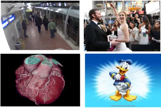
1.1 Examples of Videos. Top Left: A scene from a subway station. Top Right: A smartphone captured video. Bottom Left: Medical imaging for recording heart movements. Bottom Right: A professional movie data. . . 4

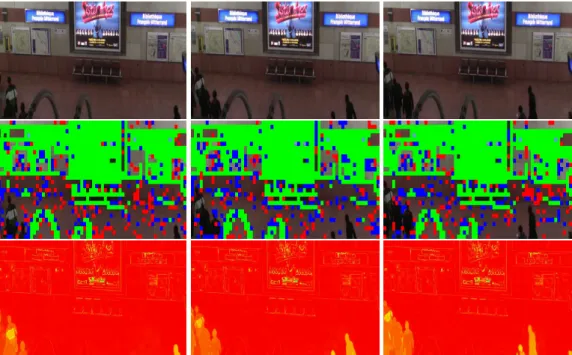
1.2 Low and mid-level vision components for an activity recognition sys-tem. First and third rows display input videos; while the second and fourth rows indicate the outputs by employing basic mid-level vision tools, namelybackground subtraction and multiple object tracking.

Col-ored blobs in the second and the fourth rows indicate different objects.

Image source: [Ryoo 2007]. . . 6

1.3 Optical Flow vectors for successive frames. The flow vectors are incorrect in the circledredzone due to lack of intensity structure. . . 7

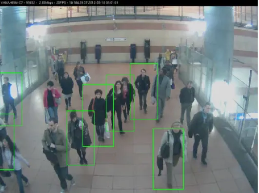
1.4 Sample detection output. Green boxes correspond to detector outputs. No-tice missed detections and impreciseness of the detector in localization of persons. . . 8

1.5 First Row: Sample input image frames from marple13 sequence by [Brox 2010]. Middle Row: A dense video segmentation. The colors rep-resent different groups. Bottom Row: A grouping of pixel trajectories (by [Brox 2010]) . White zones in images are not labeled and hence do not belong to any segments. . . 10

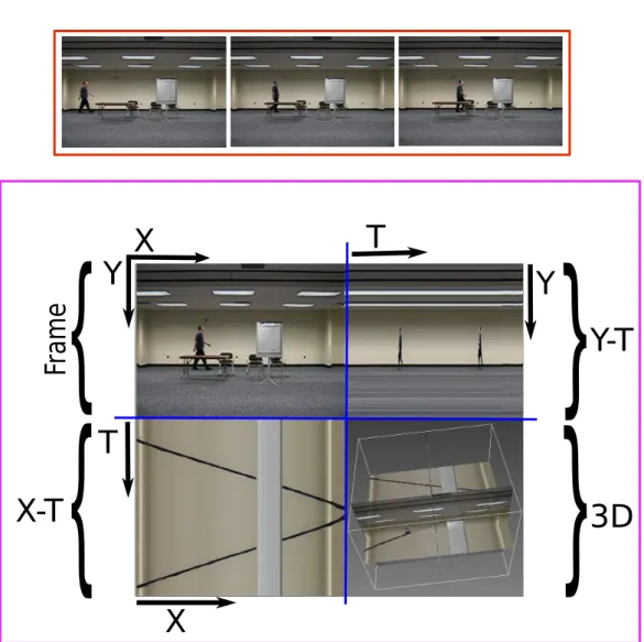
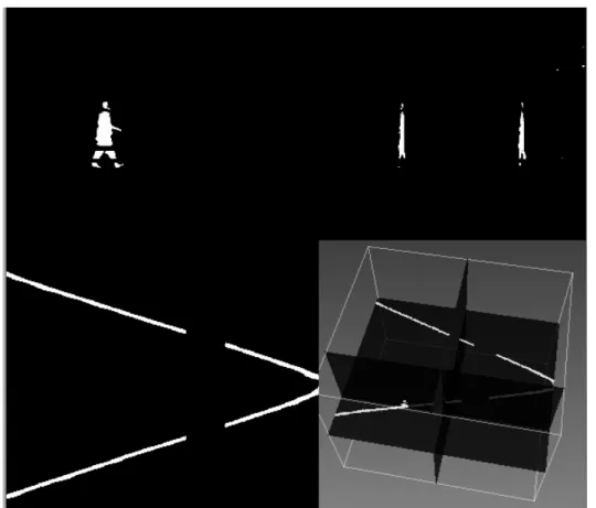
1.6 Slices of a video volume. Top row shows a few sample frames from a video. Bottom row displays the three orthogonal slices from the volume. Theblueline indicates the separation of the slices. Bottom right inset dis-plays the location of three slices inside the volume. . . 11

1.7 Deriche filter is applied on a video volume to extract the foreground (White pixels constitute the foreground). . . 12

1.8 Examples and visualization of fibers: Top Left images show a few frames from a Marple video [Brox 2010]. Top Right shows sample fibers in the first frame of the video. Bottom Row images display two snapshots from a 3D visualizer, considering the video as a 3D volume (2D+T). . . 13

2.1 An image grid with an eight-neighborhood system. . . 20

2.2 Different automatic seed selection sources. Left : Input Image. Center : Seeds obtained from homogeneity criteria. Right : Seeds obtained from edges in Input image (Seeds are shown as white regions). . . 21

2.3 Image showing the importance of non local criterion which can segment above into three regions. There are three segments in an image with a rectangular-shaped intensity ramp in the left half, a constant intensity re-gion with a hole of a high variability rectangular rere-gion.. . . 21

2.4 Segmentation result obtained by [Felzenszwalb 2004]. . . 22

2.6 Left: Braided Pattern, Right: T-Junctions (marked in red/green). . . 24

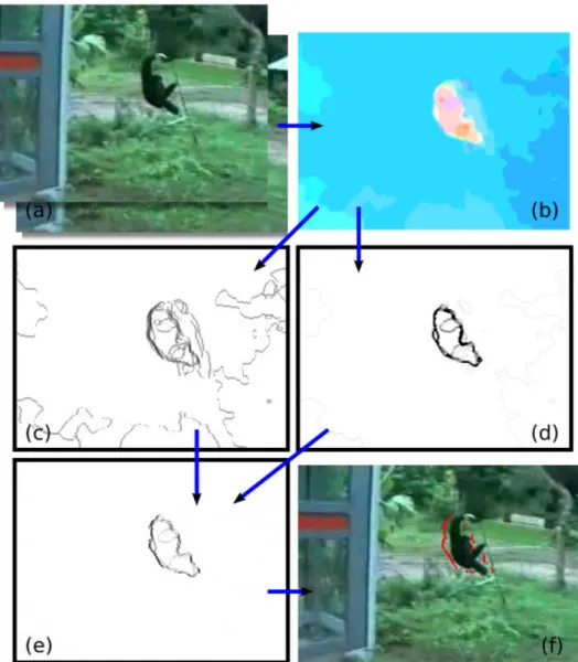
2.7 Pipeline: Object Proposal Generation by [Endres 2010]. Top Right - Bot-tom Left, BotBot-tom Right: Compute a hierarchical segmentation, generate proposals and rank proposed regions. At each stage, classifiers are trained to focus on likely object regions and encourage diversity among the propos-als, enabling the system to localize many types of objects. (Image source: [Endres 2013]). . . 26

2.8 Object proposals on a sample SegTrack video dataset (source [Tianyang 2012]). . . 26

2.9 Object proposal with objectness score. . . . 26

2.10 Segmentation results from [Tsai 2011] on the SegTrack dataset. . . 27

2.11 Motion Boundaries. (a) Two Input Frames. (b) Optical flow. The hue of a pixel indicates its motion direction and the color saturation its velocity. (c) Motion boundaries based on the gradient of the optical flow. (d) Mo-tion boundaries based on the difference in the moMo-tion direcMo-tion between a pixel and its neighbors. (e) Combined motion boundaries. (f) Final motion boundaries after thresholding. (Image source : [Papazoglou 2013]).. . . . 29

2.12 A Video grid. . . 30

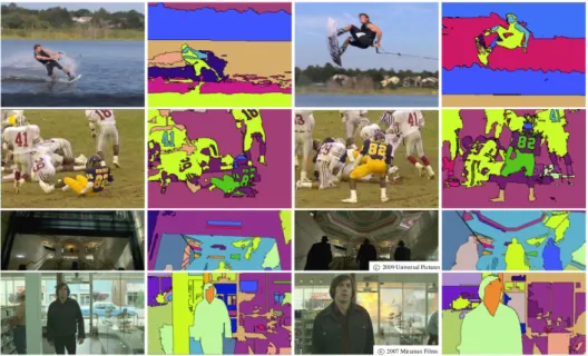
2.13 Image frames from different videos and corresponding outputs at a partic-ular hierarchy. (Image source : [Grundmann 2010]) . . . 30

2.14 First Row : Sample input image frames from marple13 sequence by [Brox 2010]. Bottom Row: A sparse segmentation obtained by group-ing of pixel trajectories (by [Brox 2010]). White zones in images do not belong to any segments. . . 32

2.15 Output from [Ochs 2011]. This approach uses the sparse labeling informa-tion from [Brox 2010] (Bottom Left) and utilizes information from super-pixels and gradients to obtain the final labeling (Bottom Right). . . 32

2.16 Background Subtraction in freely moving cameras from [Sheikh 2009]. First Row: Input image frames. Second Row: Clustered point tracks with blue representing foreground trajectories. Third Row: Estimated fore-ground labeling. Fourth Row: Groundtruth for forefore-ground separation. . . . 33

2.17 Output from [Lezama 2011]. First Row: Input image frames. Second Row: Clustered point tracks with colors denoting separate clusters. Third Row: Dense segmentation output. Fourth Row: The ground truth of ob-ject regions (left) which is automatically propagated by [Lezama 2011] to other frames (middle and right). Image Source: [Lezama 2011]. . . 34

2.18 Motion tubes based representation from [Urvoy 2009]. Image Source: [Urvoy 2009]. . . 35

2.19 Sample motion layer segmentation and relative depth ordering from [Sun 2010]. First image shows an image frame. Second image shows flow field, Third image displays the segmentation output. The colors in-dicate depth ordering with green for front, blue for middle and red for back. Detected occlusions are shown in the Fourth image. Image Source: [Sun 2010]. . . 36

3.1 2D+T video volume represented as a 3D data, as in medical imaging: frontal, sagittal and horizontal slices correspond to cuts along planes (x, y), (y, t) and (x, t) respectively. The Colored boxes around frames are in sync with the colored boxes in right bottom images. Thered linesindicate the values of x and y chosen for the cut. This video shows people exiting a train in a train station. Note in particular the lines in the (x, t) slice, formed by people trajectories, by the train or the background. We name these sets of lines fibers. . . . 41

3.2 A mesh of trajectories induces a mesh of points in each frame. . . 42

3.3 Sample fibers. Left:Redcolored patches show sample fibers on one frame. Right:Sample fibers are displayed by a 3D visualizer (ImageJ). TheGreen box encloses two straight fibers which are formed by the patches on the background. Patches forming straight fibers are marked by thebluearrows on the left image. . . 43

3.4 Straight fibers search. Left: A set of successive frames are shown, overlaid with a 2D rectangular grid. Right: A finer resolution grid is employed if the color correlation in coarser resolution grid is insufficient for building straight fibers. . . 44

3.5 Displays two straight fibers F1 and F2. Straight fibers sharing the same 2D+T cuboid and appearing at different time frames, are merged together if they are sufficiently color-correlated.. . . 45

3.6 Background fibers and the background distance map for a static camera scene. First Row: Input frames for background fiber computation. Sec-ond Row: Straight fibers. Colors indicate the length of straight fibers.

Green indicates fibers of same temporal length as that of the video. Red

colored fibers are of very short temporal length (less than 0.5 of the video temporal length). Blue colored fibers are of intermediate temporal length between the red and green fibers. Third Row: Distance map obtained af-ter extending (cf. section 3.4) onlygreen(i.e. background) fibers. The red color in this distance map indicates lower distance from the background fibers, while lighter colors indicate higher distance from the background fibers. Observe that the moving objects are at a higher distance from the background fibers, than the static regions. . . 46

3.7 Sample interest points in an image frame. We consider a high density of interest points as corner detectors in practice often miss some important corners. . . 47

3.8 Left: Corner and its neighborhood. Center: K-means in color space. Right: Spatial coherency using graph cuts.. . . 48

3.9 Flow improvement by regularizing the mesh. Left: Mt. Right:

regular-ized mesh Mt+1. The black arrow indicates the direction of the motion of

the moving object. The mesh shown is on the background and the elonga-tion of this mesh is due to the inaccurate flow near the moelonga-tion boundary of the black moving object. Green edges indicate the closing boundaries of this mesh. . . 50

3.10 Flow improvement by regularizing the mesh. Left: Mt. Right:

regular-ized mesh Mt+1. The black arrow indicates the direction of the motion of

the moving object. The mesh shown is on the background and the elon-gation of this mesh is due to inaccurate flow near the motion boundaries. Green edges indicate the closing boundaries of this mesh. . . 51

3.11 Splitting a fiber. Red and Green colors indicate separate fibers. During the fiber build process, for a certain time interval, these two fibers were considered a single fiber. Thanks to our motion coherency criteria, we detect a motion in-homogeneity at a certain time (indicated by dashed blue lines). Owing to this motion in-homogeneity detection, we split (spatially and temporally) the fiber into two, and continue the build process for each of these fibers separately. . . 51

3.12 Top Row: Displays five images of a sequence from [Brox 2010]. Bottom Row: Left image displays the same video as a 3D volume as in Fig. 3.1, with an additional bottom right corner showing the 3D position of the xt and yt slices. Right image displays all fibers found, in different colors. Notice that the fibers are well stopped near occlusion vicinity, despite high similarity in color of the tractor and the lady.. . . 52

3.13 Homogeneous and heterogeneous trajectories. The color histogram of a pixel trajectory should be as close to a Dirac peak as possible. In practice, due to some lighting variations or an imperfect camera sensor, the color histogram will not be a perfect Dirac peak. The vicinity of a histogram to a Dirac peak is quantified using the Earth Movers Distance (cf. expression 3.4). . . 54

3.14 The possible extension zone (in green) of a fiber (in brown) is projected on a reference frame (in red), following the trajectories TF

p (in blue)

associ-ated coherently with the fiber F . . . 56

3.15 Left image displays a meshed region of a fiber footprint. Right shows the distance map w.r.t. fiber. The red regions correspond to low distances, while green and blue correspond to comparatively higher distances respec-tively. Note here that the leaks are at higher distance from the sources in Red color. . . 56

3.16 Sample distance maps for fiber footprints. The Red regions correspond to low distances, while green and blue correspond to comparatively higher distances respectively. Notice that the leaks are at higher distance from the sources in Red color. . . 57

3.17 Displays extended fibers merged at a higher hierarchy. For a simple il-lustrative viewing, we fuse fibers which have similar motion. The next section 3.5 will elaborate on merging fibers. Darker regions refer to a low reliability of segmentation. . . 58

4.1 Workflow for fiber based video segmentation. . . 61

4.2 Sample frames from the dataset provided by [Grundmann 2010]. This dataset does not provide groundtruth annotations. . . 62

4.3 Sample frames from xiph.org dataset. Each row indicates three regu-larly spaced frames from a separate video. This dataset does not represent current day video usage as the frame resolution is mere 240x160, along with a poor frame rate. Importantly in many videos, there is no motion and the first and the last frames are identical (cf. last row). . . . 63

4.4 Sample video frames from the motion segmentation dataset (moseg) pro-vided by [Brox 2010]. This dataset provides pixel wise groundtruth anno-tation for a few frames in each sequence. We consider many videos from this dataset and also use their evaluation metrics (and software) to provide quantitative results. . . 64

4.5 Example from the marple3 sequence till the 50th frame. Second-Third Rows: Un-extended fibers at different hierarchy of merging. Third-Sixth Rows: Increasing hierarchy in merging of extended fibers. . . 65

4.6 First Row: Displays five images of a sequence from [Brox 2010]. Second Row: Left image displays the same video as a 3D volume as in Fig. 3.1, with an additional bottom right corner showing the 3D position of the xt and yt slices. Colored arrows on the bottom slice indicate the tractor (green

arrows) and the lady (blue arrows). Right image displays all fibers found,

in different colors. Third Row: Left image displays a high level of their hierarchical clustering. Right Image displays the highest level of the hier-archical clustering, with fiber extension. This result compares favorably to the state-of-the-art of video segmentation in Figure 4.10. . . 66

4.7 First Row: Sample input image frames (12, 24, 46, 53, 66) from marple13 sequence by [Brox 2010]. Bottom Row: After 5 steps of hierarchical merging. Parts of the foreground and background are undistinguishable during the first frames (until the 12th frame, i.e. the leftmost image in the

above figure) of the video (same color). Yet, the two objects follow later

significantly different trajectories, which enables us, when propagating this information back in time, to separate them as different fibers in all frames (cf. section 3.3.2). . . . 67

4.8 Output from [Sand 2008] dataset (frame numbers 1, 10, 20, 40). Fast mov-ing cars are appropriately segmented at a particular hierarchy.. . . 67

4.9 First Row: Sample input image frames at spacing of 40 frames till 110th frame. Second Row: Fiber merging at a lower hierarchy. Notice that the background belongs to one cluster now. Third Row: Fiber merg-ing at higher hierarchy. Notice that different parts of the movmerg-ing persons (e.g. head, torso, elbow) belong to different clusters. Fourth Row: Dense fiber flow after trajectory based association (3.4.2). Fifth Row : Extended Merged Fibers at a lower hierarchy. In this and following images, zones

segmented with low reliability are darker in color. Sixth Row: Extended

merged fibers at a higher hierarchy level. Some part of leg now belongs to the background. This due to the hierarchical merging cost function we employ. The un-extended fibers, however, have well respected boundaries as can be seen in other images. . . 68

4.10 Output from [Grundmann 2010]. Left: Input image and its spatio-temporal slices. Colored arrows on the bottom slice indicate the tractor (green

ar-rows) and the lady (blue arrows). Right: Result obtained by the

state-of-the-art segmentation of videos [Grundmann 2010], using also optical flow, for comparison. The main foreground object and the background are al-ready merged at a relatively low hierarchical level (third). It may appear that increasing the number of hierarchy levels could solve this leak. How-ever the two objects in the circled zone is of similar color and a local color & motion assessment is incapable of indicating the presence of two differ-ent objects. Our result for this video can be seen in Figure 4.6. . . 69

4.11 Sample image frames from the MPI-Sintel optical flow evaluation dataset [Butler 2012]. Each column displays consecutive image frames from one sequence. Large motion and frequent occlusions prohibit the usage of this dataset for our fiber based video representation. . . 73

4.12 Sample frames from the MIT optical flow dataset [Liu 2008]. This dataset includes groundtruth annotations.. . . 73

4.13 Optical flow computed by [Werlberger 2009] for the two consecutive frames on the left. Colors on the right image is the standard Middlebury

datasetencoding of the optical flow. We use this optical flow algorithm as

input flow for our fiber based video representation. Notice that the flow is wrongly estimated for areas between the fingers of the hand. . . 74

4.14 Interpolation of trajectories between articulated object parts. Left: A rotat-ing object part. t1 and t2mark the time instants and show poses of object.

Middle: Expected flow is shown bybluearrows. Notice that a linear inter-polation is sufficient, while a piecewise-constant interinter-polation cannot work in the case of rotations. Right: Interpolating trajectories from two trajec-tories (A, B) located at articulated object parts. . . 75

4.15 Input frames for the inpainting demo (Frame numbers: Top Row: 0, 22. Bottom Row: 44, 61). . . 76

4.16 Inpainting task. Left: original video (top) and xt slice (bottom) showing trajectories. Right: Our result. Clusters of fibers were computed and se-lected with only 7 mouse clicks to distinguish the disturbing girl from the reporter and background. The girl was removed and the hole was filled by extending the background fibers in time. . . 77

4.17 xt slices for the input (top row), and dense fibers (bottom row) at the finest hierarchy. The spatial statistics help in getting good boundary contours of the foreground object (i.e. reporter) by only a few user mouse-clicks. The straight fibers parallel to the time axis help in completing the hole formed by removing the girl. Fibers belonging to the girl are identified by finding fibers which are not parallel to the time axis. . . 77

5.1 Multiple Object (Person) Tracking. The labels for each bounding box is the unique identity of a person. Dotted points show the trajectories of bounding boxes in a few previous and successive frames. . . 82

5.2 A maximal cliques-search based tracker. Gray and colored edges repre-sent input graph and optimized subgraph respectively. Image source : [Zamir 2012]. . . 83

5.3 Network flow model graph for [Zhang 2008]. Nine detections (including false positives) from three successive frames are shown. Trajectory com-putation is performed by maximizing the flow from the source s to sink t. Nodes which are not connected (in the above Figure) to either of s, or t are deemed as false positives (post optimization) Image Source:[Zhang 2008]. 84

5.4 Higher order connections in network flow model by [Butt 2013]. Top: Graph depicting a three frame sequence with three observations in the first frame, two in the second and four in the third frame. Bottom: Graph pro-posed by [Butt 2013]. Candidate match pairs from top graph form nodes in this graph and thin black edges are added between match pairs that share an observation in frame 2, and thick colored hyperedges represent addi-tional constraints that mush be enforced so that each observation is used only once in the matching solution. Image source: [Butt 2013]. . . 86

5.5 Probabilistic Occupancy Maps. a: Original Image from three cameras. b: Probabilistic Occupancy Maps for images in above row. c: Figure represents the corresponding occupancy probabilities on the grid. Image Source:[Berclaz 2011] . . . 89

6.1 High repulsive exclusion constraints, shown for the central green bounding box in frame t, with red edges. Intra-frame exclusions prevent this detec-tion from having the same label as any other detecdetec-tion in the same frame t, while inter-frame exclusion constraints prevent it from having the same label as detections in previous and next frames t − 1, t + 1 that are too far. The maximum radius r is detection-dependent, in that it corresponds to the maximum physically-plausible displacement within a duration of one frame, and that speed estimation depends on object depth. . . 97

6.2 Point tracks and detections. . . 98

6.3 Sample Appearance Clusters for PETS09 S2L1: Each row displays a few samples belonging to the same cluster. Different sizes of cropped detec-tions indicate the distance of persons from the camera. It can be seen that the appearance features are robust to scale changes. . . 100

6.4 Computing the trajectory straightness (equation (6.1)) for a triplet of de-tections j, i, k at the temporal scale δt. . . 101

6.6 Graph reduction and flipper speed gain. Leftmost drawing shows the label-ing of 12 nodes. Node colors indicate a labellabel-ing (stuck at a local minima) and the colored lines (green and yellow) correspond to the groundtruth tra-jectories. Middle inset drawing shows the reduced graph by fusing nodes inside the dotted ellipse in the Leftmost drawing (cf. sec. 6.3.2). Since the graph is reduced, we only need to search for flips of subgraphs of size = 2 (i.e. O(|V |2_{)), instead of enumerating over all possible subgraphs of size}

= 6 (i.e. O(|V |6_{)). The subgraph-flip required to correct the initial}

label-ing is shown by magenta colored rectangular box in the middle inset. The Rightmost drawing correspond to the final correct output in the original

graph. . . 103

6.7 Illustration of the graph cleaning (cf. section 6.3.5) step. The colors of the nodes represent their associations, and same colored nodes belong to the same output trajectory. Nodes inside green boxes indicate interpolated detections for false negatives. Magenta colored nodes are false positives.. . 105

6.8 Streaming trajectory computation. Green and black colored lines repre-sents two trajectories computed in batch 1. Magenta colored nodes in the overlap time span, which belong to the same trajectory (from batch 1) are fusedtogether for batch 2. . . 106

7.1 Workflow of the proposed approach. . . 107

7.2 Model Summary. Left: Point Tracks and detections. Middle: High re-pulsive exclusion constraints, shown for the central green bounding box in frame t, with red edges. Intra-frame repulsive constraints prevent this detection from having the same label as any other detection in the same frame t, while inter-frame repulsive constraints prevent it from having the same label as detections in previous and next frames t−1, t+1 that are too far. The maximum radius r is detection-dependent, in that it corresponds to the maximum physically-plausible displacement within a duration of one frame, and that speed estimation depends on object depth. Right: Comput-ing the trajectory straightness (cf. equation (7.2)) for a triplet of detections j, i, k at the temporal scale δt. . . 109

7.3 Sample frames from the PETS dataset. . . 111

7.4 Sample frames from the TownCenter dataset. . . 111

7.5 Sample frames from the Parking Lot dataset.. . . 112

7.6 A sample frame from the PNNL ParkingLot sequence showing major deficits in the provided annotation. Besides mixing up the identities, several people are not marked in this ground truth. Image source: [Milan 2013a]. . . 113

7.7 Missing persons in annotation : Frame numbers 509 and 526 from PETS S2L1 video. The person below theredarrow is not annotated for a length of 17 frames. . . 113

7.8 Video slices along the (x, t) plane, i.e. for fixed y, for PETS S2L1, showing that labels for trajectories before and after occlusions are maintained.. . . . 115

7.9 PETS S2L1 Output: The numbers in red on each image frames show the corresponding frame numbers from this video batch. The dotted points shows the trajectories of bounding boxes in previous and successive frames. To reduce clutter in display, we show 3 trajectories and their few past and future tracks. Notice that due to the global appearance incorpora-tion, ID 4 is kept intact for the person as he leaves and comes back in the view. Also trajectories before and after crossing are fully consistent. This immaculate consistency despite False Negatives near occlusion vicinity is obtained due to the triplet factors. . . 116

7.10 Consistent people crossing. IDs 0, 11, 13, 14 (in the left part of image frames) are of interest in top rows. IDs 17 and 19’s (right part of the image frames) consistency is shown in the bottom row. . . 122

7.11 Consistent people crossing in dense scenarios. IDs 8, 9, 11, 2,3,7 are intact even after occlusion and false negatives. Images in the first row and last rows are 121 frames apart. . . 123

7.12 Iterations vs. Energy, on a problem size of 4000 variables. TRW-S is able to find usable solutions from first iteration (cf. section 7.6). . . . 124

7.13 Iterations vs. Energy. The RED line corresponds to TRW-S, while the

BLUEline corresponds to MPLP [Sontag 2012]. We observe that TRW-S is fast to minimize energy, and MPLP is unable to find one usable solution. Similar is the issue with another polyhedral method AD3 (cf. section 7.6). . 124

7.14 Processing time improvement by using graph reduction (similar MOTA in both cases), for the first 15 batches. High processing times from batch 8 to 12 are due to high detection rate/frame. In the above cases we let the optimizer run until convergence. . . 125

7.15 Average optimization processing times for the state-of-the-art tracking ap-proaches. Note that this comparison is approximate due to the reasons mentioned in section 7.7. Nevertheless there is a significant gap indicat-ing good computational efficiency of our approach. Note that we have not added the time required by the external tracker for [Milan 2013c]. . . 125

8.1 Top and Bottom Rows correspond to images from different cameras. . . 128

8.2 Correlation between a Parabola and a Line. We show that the classical covariance fails to compute any correlation, while the recently proposed

distance correlationby [Szekely 2009] computes good correlation. . . 129

8.3 Template Tracking using Covariance. Top image shows tracking with the covariance based descriptor. Bottom image shows better drift immunity by using the proposed Brownian descriptor. . . 134

8.4 Template Tracking using Covariance. Top image shows tracking with the covariance based descriptor. Bottom image shows better drift immunity by using the proposed Brownian descriptor. . . 135

8.5 Performance comparison on i-LIDS-MA [Bak 2011b].Top figure corre-sponds to N = 1, 3, while bottom figure has N = 5, 10 (cf. section 8.5 for details). . . 137

8.6 Performance comparison on i-LIDS-AA [Bak 2011b] using different met-rics: L1 corresponds to the L1norm metric between vectorized Brownian

descriptors, L1T refers to the L1 norm on a tangent plane, R - geodesic

distance [Forstner 2003] . . . 138

8.7 Performance comparison on i-LIDS [Zheng 2009]. . . 139

A.1 Difference between Dijkstra and Fast Marching Method. Image Source: http://tosca.cs.technion.ac.il/book/course_ siam10.html. . . 151 A.2 Dijkstra Algorithm. x0 is the source and hence d(x0) is zero; Set X

represents all nodes on a grid. Image Source : http://tosca.cs. technion.ac.il/book/course_siam10.html. . . 152

A.3 Algorithm Fast Marching Method. x0is the source and hence d(x0) is zero;

Set X represents all nodes on a grid. Notice the difference in the update step w.r.t. Dijkstra Algorithm in Figure A.2. Image Source : http: //tosca.cs.technion.ac.il/book/course_siam10.html. . 152

C.1 Top: A noisy image with no structure such as edges and corners. Bottom: The distribution of Ix and Iy. Both eigenvalues of T are of very small

magnitude, and hence the ellipse is of small size. . . 156

C.2 Top: An image with an edge. Bottom: The distribution of Ixand Iy. One

eigenvalue is of very large magnitude stretching one axis of ellipsoid along the corresponding eigenvector. . . 157

C.3 Top: An image with a corner. Bottom: The distribution of Ixand Iy. Both

eigenvalues are of very large value and hence the fitted ellipsoid is of larger size than in Figures C.1 and C.2 . . . 157

2.1 State-of-the-art approaches and the information provided by them. Corre-spondencescolumn indicate long term information about a pixel’s motion across the video. Dense Coverage column indicates if the segmentation approach partitions the video fully i.e. each pixel is associated to a par-ticular segment. Reliability Factor column shows if the segmentation approach provides a per-pixel factor expressing the long term quality of segmentation. . . 38

4.1 Computational time: Typical times observed for one second of a standard video, worst case times (fast background motions), and time expected if using the last GPU card and parallelization of successive chunks in a video stream on a standard 8 processor 2.4 GHz machine. . . 70

4.2 Quantitative results on the moseg dataset [Brox 2010]. Above metrics are the averaged over 15 videos (of 50 frames each). . . 71

4.3 Optical flow evaluation on the MIT dataset [Liu 2008]. Each row shows quantitative optical flow evaluation for a particular video, in terms of per pixel error, averaged over the whole sequence. . . 74

5.1 State-of-the-art approaches and their incorporation of local and global clues. TF stands for the curvature factor (triplet). GAF denotes global appearance factor. . . 91

7.1 Comparison with recent proposed approaches on PETS S2L1 Video. The metrics on the first and last row are obtained using the same code, while the middle ones are taken from the respective papers as their result files are unavailable. . . 117

7.2 Quantitative Results on Towncenter Video batch for frames 1-1000. The authors of [Benfold 2011] use information from head detector along with other information such as point-tracks to refine the locations of bounding boxes, and hence the quantity MOTP is higher. MOTA is the preferred met-ric for us as we do not make any changes in the locations of input bounding boxes, apart from adding bounding boxes for dealing with false negatives from the detector. Note that the work by [Heili 2014b] was published dur-ing this thesis completion period. . . 118

7.3 Quantitative Results on a crowded scene batch of 400 frames, starting from the 450th frame. . . 118

7.4 Quantitative Results on Parking Lot Video. Note that the groundtruth anno-tations exclude some non-occluded pedestrians and there is ID ambiguity at some frames. . . 119

7.5 Optimizer scaling w.r.t. problem size. Computation times (in seconds) for different batch sizes for PETS S2L1 video. Times in column App+k-means measure both appearance feature computation and clustering pro-cessing. For a more practical streaming trajectory computation on 50 frame batches, our optimizer takes 0.016 s/frame (on an average). Refer to the Figure 7.15 for comparative details on processing times. . . 120

7.6 Usefulness of graph reduction: PETS S2L1 computation times (in sec-onds) for the cases when the graph reduction step is either chosen (Row 1) or discarded (Row 2). The column App+k-means, shows cumulative times for both appearance feature computation and clustering. The quantitative results for both rows are similar. . . 121

7.7 State-of-the-art approaches and their incorporation of local and global clues. TF stands for the curvature penalization factor (triplet). GAF de-notes global appearance factor. . . 126

8.1 Quantitative Results for the Towncenter Video for a 390 frame batch. The first column identifies the appearance feature descriptors. . . 139

Introduction

Contents

1.1 Motivation . . . 3

1.1.1 Sources of video data . . . 3

1.1.2 Video Understanding . . . 5

1.2 Optical Flow . . . 6

1.3 Challenges for a video understanding system . . . 7

1.4 Problems Addressed . . . 8

1.4.1 Video Segmentation . . . 9

1.4.2 Multiple Object Tracking. . . 12

1.5 Contributions . . . 13

1.5.1 Video volume segmentation with Fibers . . . 13

1.5.2 Multiple object tracking using efficient graph partitioning . . . 14

1.5.3 Distance covariance based descriptor for appearance matching . . . 14

1.6 Thesis Structure . . . 14

1.1

Motivation

Video understanding is the automatic analysis and interpretation of video data. Owing to the huge amount of video data being generated everyday, an automatic video interpreter has become one of the most sought-after computer vision application.

Despite recent developments in computer vision, the maturity of video understanding systems is far from being perfect. In this thesis we address the problem of segmentation and multiple object tracking to aid video understanding. These two key problems form the core of almost all approaches for video understanding.

The following subsection presents the motivation for an automatic video understanding. Subsequently we elaborate on the building blocks that constitute most video understanding systems.

1.1.1 Sources of video data

The proliferation of cameras has driven an explosion in the amount of video data generated these days. Major contributing sources for this enormous video data are :

• Installation of security cameras at public places like streets, airports, subways. There is one camera for every 32 persons in the United Kingdom with 1.85 million cameras in function (both indoors and outdoors).

• Healthcare: During the last decade there has been a significant move towards evidence-based medicine, which involves systematically analyzing clinical data ac-quired from different sensors and making treatment decisions based on the best avail-able information. Typical application examples include videos recording movement of organs such as the heart, video data corresponding to monitoring daily livings of patients for detection of crucial diseases like Alzheimer.

• Structured and Unstructured movies: Structured video data refers to the videos cre-ated by professionals e.g. cinemas, TV shows; while unstructured corresponds to data created by general public. With the decrease in prices of smartphones & con-sumer cameras, coupled with a steep increase in social media interaction, there has been a burst in the creation of unstructured data. One of internet’s major video data provider Youtube gets uploaded with 48 hours of video everyday. Images and videos altogether comprise 80% of all corporate and public unstructured big data.

Figure 1.1: Examples of Videos. Top Left: A scene from a subway station. Top Right: A smartphone captured video. Bottom Left: Medical imaging for recording heart move-ments. Bottom Right: A professional movie data.

Figure1.1 shows typical sources for video data. Owing to this huge amount of video data, there is a pervasive need in any sector (industry, government) to analyze these data automatically. The enormousness of this data also presents challenges to create efficient storage hardware and software, which is a driving force behind research in data

compres-sion and related hardware. Automatic analysis of video (i.e. video analytics) data can help prescribe actions which in-turn will improve health care, reduce crime, and so on.

1.1.2 Video Understanding

Video understanding is the automatic and logical analysis of information found in the video data. An example of an understanding system is a people counter at supermarkets which could help managing customer services at tills efficiently. On a computer, images are rep-resented as vector images or raster images. Raster images are sequences of pixels with discrete numerical values for color while vector images are a set of color annotated poly-gons. A video is a sequence of images. In order to extract logical information from videos, the encoding must be transformed into constructs depicting physical structures, objects and motion. These constructs will then be analyzed by the computer.

In order to understand the typical building blocks of a video understanding system, let us consider the workflow of an activity recognition system. The aim of an activity recognition system is to automatically label objects, persons and events in a given video. Activity recognition is an important research domain in computer vision and its application areas include surveillance systems, healthcare monitoring, human-computer interactions. Automated surveillance systems in public places such as streets, airports, subways aim at detecting abnormal and suspicious activities. Another important usage of activity recogni-tion is in automatic monitoring of patients and elderly human beings.

Owing to the importance of the task of activity recognition, numerous approaches are being proposed every year at major computer vision conferences. However the accuracy of these systems are far from being perfect. The major limiting factor for good performance of an activity recognition system is the unreliability of low and mid level computer vision components. Low-level vision refers to processing of an image or a video for extracting primitive features such as color edges or corners. Mid-level vision tasks use inputs from low-level vision algorithms to accomplish tasks such as estimation of 3D scene properties from 2D images, determining camera motion from videos and segmentation of an image (or video) into coherent subsets. The automatic interpretation of the information provided by low and mid level vision for conceptual description of the scene (e.g. activity recognition) is referred to as high level vision.

The low and mid level vision components form building blocks for high level vision tasks such as activity recognition. Figure1.2displays sample outputs after a low and mid level processing of the input video. This processing is required for the task of human-object interaction (picking a trash-can or moving hand-luggage). Given an input video, object hypotheses are obtained on a per-frame basis. This task is commonly referred to as

object detection. Often algorithms such as background removal is employed in order to

boost the accuracy of object detection algorithms. A background removal aids an object detection algorithm in removing the noisy outputs which are on high probable background regions.

Subsequently, in order to detect activities performed by objects, the requirement is to infer the motion of the objects in the scene. This task of computing motion of objects in a scene by associating detection hypotheses in image frames is known as Multiple Object

Figure 1.2: Low and mid-level vision components for an activity recognition system. First and third rows display input videos; while the second and fourth rows indicate the outputs by employing basic mid-level vision tools, namelybackground subtraction and multiple

object tracking. Colored blobs in the second and the fourth rows indicate different objects.

Image source: [Ryoo 2007].

Tracking. The second and fourth row in Figure1.2 show outputs after performing

back-ground removal and object tracking on the input video.

Recognition of tasks such as picking a hand-luggage or placing a box in trash-can (cf. Figure1.2) require details about movement of the hand and pixels constituting the hand. This is accomplished by computing trajectories of pixels belonging to the hand. Trajectory of a pixel refers to a time ordered set of points which determine its temporal movement across the video.

An activity recognition approach exploit the above low and mid-level vision informa-tion to recognize activities in a video. Typically this step involves statistical pattern recog-nition algorithms to model the relationship between activities and the basic information obtained from low and mid-level vision tasks.

1.2

Optical Flow

Before we delve any further, it is important to mention one of the important concepts, namely optical flow, which forms the basis for motion computation of pixels in videos, and is used in almost all video understanding systems. Optical flow is the distribution of apparent velocities of movement of brightness patterns in an image [Horn 1981]. Optical flow computing algorithms input a pair of consecutive image frames (one as source and another as target), and provides apparent motion estimates for each pixel from the source

Figure 1.3: Optical Flow vectors for successive frames. The flow vectors are incorrect in the circledredzone due to lack of intensity structure.

image to the target image. Several techniques for computing optical flow exist in the liter-ature. However the accuracy is very limited due to practical difficulties in estimating large displacements for pixels. Moreover it is difficult to compute reliable flow vectors in homo-geneous color areas. The red zone in Figure1.3shows inaccuracy in optical flow vectors inside the red colored elliptical zone. Notice that the flow vectors are of much higher accu-racy near corners and edges. The flow at corners are more reliable due to lesser ambiguity in matching corners in successive frames. The flow ambiguity at edges is also referred as the aperture problem in the literature.

1.3

Challenges for a video understanding system

In the previous sections we have seen some basic vision components used for recognizing activities. The information obtained from the low and mid level vision component is also referred to as features, in the computer vision literature. The features are encoded into suitable descriptors. The features and their descriptions need to be carefully chosen so that they encode definitive information regarding the presence of activities.

Figure 1.4: Sample detection output. Green boxes correspond to detector outputs. Notice missed detections and impreciseness of the detector in localization of persons.

Video understanding is challenging due to unreliable outputs provided by basic low and mid-level vision algorithms such as optical flow, object detection. Another challenge for a video understanding system lies in building tractable models for relating features and objectives.

In an earlier section we have seen the inaccuracy of motion estimates provided by optical flow, which impairs the computation of dense and accurate trajectories for pixels in the video. This in-turn limits the amount of reliable temporal information available for video understanding.

Figure 1.4 shows the output from another important lower level vision component, namely an object detector, for a video understanding system. A person detector is employed to obtain detection hypotheses on the image frame shown in Figure 1.4. The detections obtained by the person detector are shown by the rectangular boxes. Notice that many persons are not detected by the detector, and the localization of some persons are poor. This impreciseness of an object detector pose serious challenges to the tracking of objects, and further limits the accuracy of an understanding system requiring an object tracker.

1.4

Problems Addressed

In this thesis we aim to improve the key mid-level vision components, namely video

A segmentation algorithm provides detailed spatio-temporal relationships of pixels in a video, which are necessary to analyze the geometry and shape changes of object/object-parts across time and space. Another important component of a video understanding sys-tem is a multiple object tracker which provides spatio-sys-temporal movement details about objects in a scene. This output provided by a multi-object tracker is at an object level and hence detailed movements of pixels comprising objects is not available. On the other hand segmentation algorithms, generally do not provide a notion of objects in the outputs. Seg-mentation algorithms which provide semantic label for each pixel of a video are referred to as semantic segmentation methods.

A good segmentation and multi-object tracking for a video understanding system aids in the extraction of reliable features. This subsequently helps in modeling robust relation-ships between features and output variables. In this thesis we address both these problems, namely video segmentation and multiple object tracking.

1.4.1 Video Segmentation

A segmentation algorithm partitions an input video into several components. Each com-ponents is homogeneous w.r.t. one or more properties i.e. the variation of measurements within the regions should be considerably less than variation at the object borders.

Numerous segmentation algorithms exist in the literature. Also any particular segmen-tation approach cannot be suitable for all video understanding tasks. About 30 novel seg-mentation approaches get published at a major computer vision conference, underlining the hunch for a reliable segmentation approach. However a reliable and robust segmentation still eludes the vision community.

The requirements for segmentation depends on the video understanding task. Moreover there can be different segmentation algorithms catering to the same video understanding task. A people counting system may use a motion based segmentation or a segmentation based on filters whose response can localize the persons in a video.

Video segmentation approaches can be broadly classified into two categories, based on the impetus on color on motion information to obtain a segmentation :

• Color based : Approaches belonging to this category primarily rely on color of the pixels to perform segmentation.

• Motion based : Motion provides vital clues for grouping and algorithms under this category rely mainly on motion information to achieve segmentation. Owing to the difficulty in extraction of motion at color homogeneous regions, many algorithms belonging to this category can provide grouping of only a subset of pixels in a video. The last row in Figure 1.5 shows an example for sparse motion based grouping. This grouping has little or no spatial coherency in the output. Typically these sparse representations provide grouping for a mere subset of 3 to 5% of the total pixels in the video.

Most segmentation approaches use a combination of both motion and color informa-tion. However the segments obtained are 2D+time (3D) blobs, termed as supervoxels,

Figure 1.5: First Row: Sample input image frames from marple13 sequence by [Brox 2010]. Middle Row: A dense video segmentation. The colors represent differ-ent groups. Bottom Row: A grouping of pixel trajectories (by [Brox 2010]) . White zones in images are not labeled and hence do not belong to any segments.

which provide little or no detail about spatio temporal motion about pixels constituting the blobs.

The proposed approach in this thesis uses both color and motion information to segment a video. In contrast to the existing state-of-the-art segmentation approaches, we aim at building long term spatio-temporal movement details for all pixels in the video.

Most of the segmentation approaches proposed until the early 2000s are based on frame-by-frame processing. Recently, with the increase in computational efficiency of computers, there is an emerging trend to compute representations based on stacking multi-ple successive frames (in the order of hundreds) of the video. We term this stack video vol-umes. Volume-based approaches have gained importance, as jointly processing all frames of a video brings more information and helps maintaining a coherent segmentation over time. Figure1.6shows slices of a video volume formed by stacking 100 successive frames. In this figure, the first row indicates sample frames of a video. The lower image (inset) dis-plays the video volume by it’s three orthogonal slices (cf. caption for more details).

On this video volume, one of the simplest segmentation task could be to extract fore-ground by computing edges in the temporal (T) dimension. The intuition is that for a fixed camera video, if a person is walking perpendicularly to the camera’s optical axis with suf-ficient speed, then the pixels corresponding to the edges will belong to the person. To this end we use the Deriche filter [Deriche 1987] for computing edges along the temporal axis. This filtering is followed by a thresholding step wherein sufficiently strong-valued edges are kept and the rest are suppressed (dark zones in Figure1.7). Thus we now obtain a bi-nary labeling of the video wherein the foreground corresponds to the white zones in Figure

1.7. The high coherency in background labeling is due to jointly processing the 2D+T data in the form of a video volume. This joint processing helps an edge detector to localize

X-T

Y-T

Fr

am

e

X

Y

X

T

Y

T

3D

Figure 1.6: Slices of a video volume. Top row shows a few sample frames from a video. Bottomrow displays the three orthogonal slices from the volume. Theblueline indicates the separation of the slices. Bottom right inset displays the location of three slices inside the volume.

edges in a better way than considering only two successive frames.

Another advantage brought by this volume is long temporal range information. Local motion information among spatially neighboring pixels can be inaccurate as shown in Fig-ure1.3. However modeling long term affinity (with suitable criteria) between pixels could help in getting around this problem in color homogeneous regions. With reference to the example in Figure1.3, a viable approach to build accurate flow in red zones (lacking dis-criminative intensity structure) is to propagate the high accuracy flow from the edges and corners on the moving person.

In this thesis we pursue video volumes to obtain a robust, reliable and dense video segmen-tation along with long range motion estimate for each pixel in the video.

Figure 1.7: Deriche filter is applied on a video volume to extract the foreground (White pixels constitute the foreground).

1.4.2 Multiple Object Tracking

The task of multiple object tracking refers to the detection and tracking of moving objects (of a particular category) in a scene. This task is usually tackled in two steps :

• Detecting Objects : An object specific detector is applied to obtain detection hy-potheses in a video.

• Data Association : Detection hypotheses are associated to compute trajectories for objects. An object trajectory refers to a time ordered set of object detections. In this thesis, we focus on the data association aspect of a multiple object tracker.

Video volume opens up new perspectives in object tracking. Recent tracking ap-proaches in the state-of-the-art report the usefulness of video volumes in managing oc-clusions and maintaining precise trajectories for objects.

Figure 1.4 shows an object detector’s response (a.k.a. detection hypotheses) on an image frame. Spurious and missed detections along with imprecise localizations are the main challenges for multiple object tracking. Detection hypotheses form interesting spatio-temporal patterns (e.g. cliques in [Zamir 2012]) and in the recent past there has been an increase in interest in finding these patterns to compute object trajectories.

We address the problem of object tracking by utilizing the spatio-temporal structure around the detection hypotheses.

1.5

Contributions

This thesis brings out the following contributions : 1.5.1 Video volume segmentation with Fibers

Figure 1.8: Examples and visualization of fibers: Top Left images show a few frames from a Marple video [Brox 2010]. Top Right shows sample fibers in the first frame of the video. Bottom Rowimages display two snapshots from a 3D visualizer, considering the video as a 3D volume (2D+T).

With respect to the state-of-the-art in video segmentation, the two contributions are as follows :

• We combine both spatial and temporal aspect of video into a single notion, Fiber. A fiber is a set of trajectories spatially connected by a triangular mesh. Some examples

of sparse fibers can be seen in Figure1.8. Fibers are a mid level entity and serve the purpose of bridging the gap between low-level pixels and high-level activity recog-nition.

• Another contribution is the incorporation of hierarchical clustering into segmenta-tion, with meshes. For domains like action recognisegmenta-tion, it is often desired to keep the finest representation in term of fibers (long term dense optical flow) while for domains like background segmentation or foreground estimation (in freely moving cameras) a much coarser representation can be selected.

1.5.2 Multiple object tracking using efficient graph partitioning

Another contribution of this thesis is in the domain of multiple object tracking. We conduct trajectory computation on a video volume. An off-the-shelf person detector is used to obtain probable locations of persons for all frames of this volume. A graph is formed with detections hypotheses as the nodes, and suitable edges are incorporated to encode suitable affinity functions using spatio-temporal cues. The multi-object tracking is then modeled as a graph partitioning problem, such that a part corresponds to trajectory of a person.

This thesis brings out following contributions in this domain :

• Formulating tracking as an energy minimization problem, wherein the natural con-straints of object tracking are dealt in a principled manner.

• A computationally efficient combination of optimizers to achieve a near real time tracking performance, along with maintaining competitive results with the state-of-the-art.

1.5.3 Distance covariance based descriptor for appearance matching

A minor contribution of this thesis is in developing a novel descriptor for appearance matching. We consider the task of identifying persons across multiple cameras. This task is popularly known as identification. Appearance matching for the person re-identification is often based on the covariance of several features such as intensity, gra-dients and wavelets. However the covariance matrix C(X,Y) cannot express reliable corre-lations if the random variables X,Y are non-linearly dependent. Recently [Szekely 2009] proposed a novel coavriance measure termed Distance Correlation, which can compute all degrees of possible relationships between random variables. We proposed a descrip-tor based on distance correlation which outperforms previous state-of-the-art covariance descriptors on re-identification datasets.

1.6

Thesis Structure

This complete thesis is divided into three parts. The first part provide details about Video

The final part concludes this thesis by summarizing the contributions and indicating future research directions.

The chapters are organized as follows:

Chapter 1introduces the motivation and objective of this thesis.

Part 1: Video Segmentation

Chapter 2provides an overview of the state-of-the-art in video segmentation.

Chapter 3describes the first major contribution of this thesis i.e. video segmentation using

Fibers.

Chapter 4 presents quantitative and qualitative evaluations, and comparisons with the state-of-the-art for video segmentation using fibers.

Part 2: Multiple Object Tracking

Chapter 5outlines state-of-the-art approaches in multiple object tracking.

Chapter 6describes the second major contribution in the domain of multi-object tracking. Chapter 7presents qualitative and quantitative results along with comparisons from state-of-the-art for multiple object tracking.

Chapter 8provides detail on appearance matching using distance correlation. This chapter will conclude with quantitative results and discussions on the appearance descriptor applied to tracking and Re-Identification.

Part 3: Concluding the thesis

Chapter 9concludes this thesis by outlining future research directions and perspectives on video segmentation & multiple object tracking.

Video Segmentation: Related Works

Contents

2.1 Image Segmentation . . . 20

2.1.1 Seeded Region Growing . . . 20

2.1.2 Graph Based Image Segmentation . . . 21

2.1.3 Superpixels . . . 23

2.2 Video Segmentation without correspondences. . . 23

2.2.1 Segmentation with Object Proposals . . . 24

2.2.2 Hierarchical graph based video segmentation . . . 28

2.3 Video Segmentation with correspondences . . . 31

2.3.1 Clustering of Point Tracks . . . 31

2.3.2 Point Tracks and Hierarchical Video Segmentation . . . 34

2.3.3 Tube or mesh based video representation . . . 35

2.3.4 Motion layer segmentation . . . 35

2.4 Conclusion . . . 37

Video segmentation has been an active area of research since 1980s. Current work on video segmentation can be broadly classified into two categories: frame-by-frame based approaches and volume-based approaches. Frame-by-frame approaches take as input one or two successive frames of a video, while volume-based approaches consider many suc-cessive frames of a video at once. Frame-by-frame approaches have the advantages of low memory requirement while volume-based approaches in recent years have demonstrated good coherency in object labeling over time. Frame-by-frame approaches are also termed as streaming algorithms as they can be directly applied to a video stream. Recently with the increase in computers’ memory, volume-based approaches have gained importance, as jointly processing all frames of a video brings more information and helps maintaining segmentation or trajectory coherency over time. However the accuracy of current video segmentation algorithms still needs to be improved.

Video segmentation approaches combine various cues from motion, color, to provide spatially and temporally coherent output. An object or part of an object in a video can be identified based on the similarity of color. However the presence of texture, or inhomo-geneous appearance of objects e.g. persons wearing different shaded clothing, adds to the complexity in analyzing the extent of objects. In these cases temporal information from various frames of a video can be exploited to identify the object or its parts. For example

an object in a scene with similar color as the background can be identified based on the difference in motion w.r.t. background.

Motion provides vital cues regarding the grouping of pixels, and the existence of similar motion for pixels implies their similar fate i.e. similar grouping (Gestalt principle).

A key component for many vision algorithms is the estimate of long term correspon-dences for pixels in a video. This long term correspondency for a pixel is also referred to as point trajectory in the computer vision literature. Dense point trajectories are required for finely analyzing the videos. For example, a gesture recognition system characterizing different hand movements will require temporal details about the movement of the hand,

i.e. long term correspondences for pixels constituting the hand. A video segmentation

algorithm can be broadly categorized into two classes depending on the motion estimates provided:

• Segmentation without correspondences: Approaches belonging to this category pro-vide grouping of pixels as objects or object-parts across the pro-video. This grouping provides no detail about long term motion of components (pixels) constituting the group. In plus of color information, most of these approaches use local motion infor-mation computed from optical flow. These algorithms are sought out for application like video tooning, object extraction.

• Segmentation with correspondences: These approaches provide trajectories for most pixels of the video. Application areas include activity/gesture recognition, video compression, object extraction.

2.1

Image Segmentation

Before we delve into video segmentation approaches, it is important to mention some reli-able image segmentation techniques which form the basis for several state-of-the-art meth-ods in video segmentation.

2.1.1 Seeded Region Growing

Figure 2.1: An image grid with an eight-neighborhood system

A region growing approach starts with an incomplete segmentation (i.e. set of regions which does not cover the full image) and attempts to aggregate the unlabeled pixels to one of the regions. The initial set of regions are also known as seeds. A pixel is merged

Figure 2.2: Different automatic seed selection sources. Left : Input Image. Center : Seeds obtained from homogeneity criteria. Right : Seeds obtained from edges in Input image (Seeds are shown as white regions).

to a seed if it fits a predefined criterion based on color similarity. Seeds can either be found manually or in an automatic manner. In manual seed selection, a user annotates the object or its parts by scribbles. On the other hand, an automatic selection of seeds can be performed by information from image gradients, edges as performed by [Köthe 1995]. Some automatic seed selection techniques are shown in Figure2.2. Once these seeds are located, optimization approaches like Dijkstra [Köthe 1995] or graph cuts [Boykov 2006] can be employed to obtain the final segmentation.

2.1.2 Graph Based Image Segmentation

The core motive of this work is in finding criteria which define non local characteristics of an image.

Figure 2.3: Image showing the importance of non local criterion which can segment above into three regions. There are three segments in an image with a rectangular-shaped intensity ramp in the left half, a constant intensity region with a hole of a high variability rectangular region.

Unlike the classical methods in image segmentation (such as split and merge), this method adaptively adjusts the segmentation criterion based on the degree of variability in neighboring regions of the image. This results in a method that, while making greedy decisions, can be shown to obey certain non-obvious global properties. Figure 2.3 from

[Felzenszwalb 2004] shows that a purely local criteria is insufficient to distinguish the three regions. Specifically, in order to obtain a segmentation of the image in Figure2.3, breaking edges with large color variations will never be able to find a segmentation of the high variation region on the right.

Another important aspect of this work is its computational efficiency. The complexity of the approach is quasilinear i.e. O(ElogE), where E is the number of edges. Hence this approach is practically more amenable than its counterparts in image segmentation e.g. Normalized cuts by [Shi 2000] whose complexity is quadratic in terms of number of edges of the graph.. A sample output from this segmentation algorithm is shown in Figure2.4.

Figure 2.4: Segmentation result obtained by [Felzenszwalb 2004].

Implementation

An image is viewed as a graph (V, E), where vertices (or nodes) V correspond to the pixels of an image and edges E are defined by four or eight neighborhood connectivity, as shown in the Figure2.1. Edges are weighted according to the color difference between the nodes they connect. The segmentation process begins with the completely disconnected graph, edges are added one at a time in increasing order of their weights. Prior to adding an edge, there are as many connected components as the number of pixels in the image. An edge addition decreases the number of connected components. The process maintains a forest of Minimum Spanning Trees (MST) for the current components. During an edge addition, each MST Ciis associated with a threshold T (Ci) = w(Ci) + k/|Ci|, where w(Ci) is the maximum weight in the spanning tree of the component Ciand k > 0 is a constant.

An edge e, whose endpoints belong to the different components Ciand Cj is added if and only if

w(e) <= min(T (Ci), T (Cj)), where w(e) is the weight of the edge.

This process is a reminiscent of the famous Kruskal’s Minimum Spanning Tree algo-rithm. The parameter k for fusing nodes (or adding edges) can be varied to obtain hierar-chical segmentation outputs ([Grundmann 2010]). At the lowest level (small value for k) in the hierarchy, an image is segmented to many regions and the number of regions decreases by increasing the value of k.

2.1.3 Superpixels

Superpixels are atomic clusters of pixels which are perceptually meaningful. Superpixel computation has become an important pre-processing step for several image processing and vision tasks. Instead of working on a large graph of pixels, many high level inference tasks extract superpixels in an image to reduce the size of the problem. This provides a significant gain in speed as the number of superpixels for an image is typically 1000 times lesser than the number of pixels. Notice that the lowest level hierarchy (if appropriately chosen) of the approach by [Felzenszwalb 2004] can also provide superpixels.

One of the most popular superpixel algorithm is by [Achanta 2012] and is referred to as SLIC superpixels. Sample images from SLIC are shown in Figure2.5.

Figure 2.5: Sample superpixels from [Achanta 2012] of sizes 64, 256 and 1024.

2.2

Video Segmentation without correspondences

Each moving part of an object carves a distinct sub-volume in the 2D+T cube formed by the video. A viable approach for segmentation would be to directly extract or model these sub-volumes. [Niyogi, S.A. and Adelson 1994] is one of the first works on analyzing the