HAL Id: tel-01104818
https://hal.archives-ouvertes.fr/tel-01104818
Submitted on 19 Jan 2015HAL is a multi-disciplinary open access
archive for the deposit and dissemination of sci-entific research documents, whether they are pub-lished or not. The documents may come from teaching and research institutions in France or abroad, or from public or private research centers.
L’archive ouverte pluridisciplinaire HAL, est destinée au dépôt et à la diffusion de documents scientifiques de niveau recherche, publiés ou non, émanant des établissements d’enseignement et de recherche français ou étrangers, des laboratoires publics ou privés.
Public Domain
TECHNIQUES FOR MULTIUSER MIMO
BROADCAST CHANNELS
Lei Zhao
To cite this version:
Lei Zhao. BEAMFORMING AND POWER ALLOCATION TECHNIQUES FOR MULTIUSER MIMO BROADCAST CHANNELS. Engineering Sciences [physics]. UNIVERSITE DE NANTES, 2014. English. �tel-01104818�
Thèse de Doctorat
Mémoire présenté en vue de l’obtention
du grade de Docteur de l’Université de Nantes Sous le label de l’Université Nantes Angers Le Mans
Discipline : Electronique
Spécialité : Communications numériques Laboratoire : IETR UMR 6164
Soutenance le 1er octobre 2014
École doctorale Sciences et Technologies de l’Information et Mathématiques (STIM)
JURY
Président : M. Salah BOURENNANE, Professeur, Institut Fresnel, Ecole Centrale Marseille Rapporteurs : M. Gilles BUREL, Professeur, Université de Bretagne Occidentale, Brest
M. Jean-Pierre CANCES, Professeur, Université de Limoges
Examinateurs : M. Guillaume ANDRIEUX, Maître de Conférences, IUT La Roche s/Yon Directeurs de Thèse : M. Pascal CHARGE, Professeur, Ecole polytechnique de l’université de Nantes M. Yide WANG, Professeur, Ecole polytechnique de l’université de Nantes
ED-503
Lei ZHAO
B
EAMFORMING AND
P
OWER
A
LLOCATION
T
ECHNIQUES
FOR
M
ULTIUSER
MIMO
B
ROADCAST
C
HANNELS
Acknowledgments
First and foremost, I would like to express my deepest gratitude to my supervisor Prof. Chargé and co-supervisor Prof. Wang, for their professional guidance and un-conditional support throughout the entire three years of my PhD study. I thank them for the countless hours they spent discussing my research work, giving professional suggestions, and correcting the manuscripts. I also thank them for giving me a down-to-earth attitude and spirit in my future career.
Of course, I have to thank my friends and every colleague in the lab, for making these three years in France so enjoyable.
In addition, I would also like to thank China Scholarship Council (CSC) for the financial support.
I also want to express my gratitude to my parents, for their selfless support, I cannot imagine coming so far without their love and understanding.
Finally, I thank my girlfriend Han Zheng for her sweet and thoughtful love, which has substantially supported me for my PhD study.
Résumé de la thèse en français
Pour augmenter les débits de transmission, de nouvelles techniques permettant d’améliorer l’efficacité spectrale des systèmes de télécommunication sont proposées. Parmi les techniques prometteuses, Multiple-Input Multiple-Output (MIMO) est très étudiée [1], [2]. La technique MIMO permet en effet de transmettre plusieurs symboles de données différents de manière simultanée et sur la même bande de fréquence. Cette technique a d’abord été étudiée pour des liaisons point-à-point, c’est-à-dire entre un émetteur et un récepteur, chacun équipé de plusieurs antennes. Les travaux [3], [4] et [5] indiquent notamment que l’efficacité spectrale obtenue pour des systèmes équipés de plusieurs antennes peut s’avérer importante lorsque le canal offre beaucoup de di-versité. Dans [6] et [7] les auteurs soulignent que pour un canal à bruit additif gaussien indépendant et identiquement distribué, la capacité des systèmes MIMO peut croître linéairement avec le nombre d’antennes de transmission ou de réception.
Depuis quelques années, une extension de MIMO nommée multi-utilisateurs MIMO (MU-MIMO) attire de plus en plus d’attention par rapport au système MIMO clas-sique. MU-MIMO permet en effet d’établir des communications simultanées avec plusieurs utilisateurs répartis dans l’espace, chacun équipé d’antennes multiples. Ce système permet donc de servir simultanément plusieurs utilisateurs avec une grande efficacité spectrale en exploitant la diversité spatiale. Ce service est possible au prix d’un traitement du signal plus intensif [8], [9]. Le schéma de base est celui d’une station de base en lien avec plusieurs utilisateurs simultanément dans la même bande de fréquence, et qui exploite les différentes signatures spatiales induites par la disper-sion géographique des utilisateurs. Cette technique est également connue sous le nom de Space-Division Multiple Access (SDMA) [10]. Il est montré qu’en appliquant la technique DPC (Dirty-Paper-Coding), le système MU-MIMO a la capacité d’annuler les interférences connues non causalement au niveau de l’émetteur. A l’aide de tech-niques de formation de voies, il est possible de supprimer les autres interférences. La formation de voies a été utilisée dans les systèmes MIMO [11] de manière optionnelle pour améliorer le rapport signal-sur-bruit (RSB) au niveau du récepteur [12]. Afin
de profiter pleinement de l’amélioration des performances apportée par le multiplex-age spatial dans les systèmes MU-MIMO, les techniques de formation de voies sont essentielles pour éliminer ou minimiser les interférences multi-utilisateurs (MUI).
Le chapitre 2 introduit les canaux MIMO, MU-MIMO, et les canaux d’accès mul-tiple (MAC). La liaison descendante, de la station de base avec des antennes mulmul-tiples vers plusieurs utilisateurs, chacun étant équipé d’une ou de plusieurs antennes, est définie comme un canal de diffusion MU-MIMO. L’objet de l’étude est de déterminer la formation de voies optimale en termes de capacité de ce système. S’agissant ici d’un problème d’optimisation non convexe et non-concave [13], la dualité entre le canal de-scendant MU-MIMO de diffusion et le canal MAC de liaison montante est exploitée. Cependant, malgré l’exploitation de cette propriété, la complexité reste élevée pour résoudre le problème. Afin de réduire cette complexité, des méthodes sous-optimales telles que ZF-DPC [14], SA-DPC [15] et SBD-DPC [16] ont été proposées. Pour ce type de méthodes qualifiées de non linéaires, les signaux à transmettre sont générale-ment encodés d’une manière séquentielle. On distingue alors à chaque étape, une partie de l’interférence, connue au niveau de l’émetteur, et étant causée par les signaux précédemment encodés. Cette interférence peut être éliminée simplement par la tech-nique DPC. Ceci offre plus de degrés de liberté pour la détermination des vecteurs de formation de voies à l’émission, puisqu’il reste à annuler uniquement la partie restante de l’interférence. Cette stratégie conduit généralement à des performances importantes en termes de débit pour ces méthodes non linéaires. La méthode ZF-DPC ne permet de considérer qu’une seule antenne de réception par utilisateur, tandis que la méthode SBD-DPC permet de considérer plusieurs antennes de réception par utilisateur. La méthode SA-DPC proposée dans [15] détermine la formation de voies en émission et en réception pour les flux de données d’une de manière séquentielle. Cette méthode fonctionne même si le nombre total d’antennes en réception est supérieur au nombre d’antennes à l’émission. Un aperçu de ces techniques d’optimisation non-linéaires nécessitant l’algorithme DPC, est donné dans le chapitre 3.
Bien que la capacité globale fournie par ces dernières méthodes s’approche de la capacité optimale, elles nécessitent la mise en œuvre de l’algorithme DPC qui aug-mente la complexité. Par conséquent, des solutions de traitement linéaires, telles que la méthode ZF [17], la méthode BD [18], la méthode RBD [4], la méthode CB [19] et la méthode ZF-SA [20] ont été proposées. Ces méthodes permettent aussi d’annuler complètement l’interférence par la formation de voies. Les méthodes ZF et BD con-sistent, pour chaque utilisateur, à trouver un vecteur de formation de voies à l’émission orthogonal à l’espace formé par les autres utilisateurs. Les méthodes ZF-SA et CB
7 permettent de considérer les cas où le nombre total d’antennes en réception est plus grand que le nombre d’antennes à l’émission. La condition de ZF est relaxée dans la méthode MMSE [21], et les vecteurs de formation voies à l’émission sont calculés par les valeurs propres généralisées. Toutes ces techniques sont décrites dans le chapitre 3. La mise en œuvre de ces méthodes reste raisonnable en termes de complexité. Cepen-dant pour toutes ces techniques, l’optimisation se fait sous une contrainte de puissance cumulée.
Dans la pratique, chaque antenne émettrice possède un amplificateur de puissance dont la linéarité est nécessairement limitée; en particulier dans le cas du système OFDM qui présente de forts PAPR [22]. Ainsi, il est plus réaliste de chercher à opti-miser le débit avec une contrainte de puissance non plus totale mais relative à chaque antenne d’émission. Des techniques de formation voies avec une contrainte de puis-sance par antenne ont été étudiées dans [23], [24], [25], [26] et [27]. Les travaux [23] et [24] se placent dans le cas où chaque utilisateur est équipé d’une seule antenne et considèrent un pré-codage de ZF. Dans [25] cette contrainte ZF est relaxée. Dans [26] les auteurs analysent le cas où chaque utilisateur est équipé de plusieurs antennes, et l’algorithme DPC est utilisé en considérant un ordre d’attribution prédéfini des util-isateurs. Cette méthode [26] attribue à chaque utilisateur un certain nombre de flux de données en fonction du rang de sa matrice de canal. Ce dernier point n’est cepen-dant pas optimal car les canaux offrant un débit faible ou même négligeable pour un utilisateur pourraient introduire néanmoins de fortes contraintes pour les autres utilisa-teurs [15]. Dans [27], la solution optimale sous contrainte de puissance par antenne est obtenue par l’exploitation de la dualité des canaux montants et descendants. Les techniques mises en œuvre pour résoudre ce problème d’optimisation convergent mal-heureusement assez lentement [25]. L’état de l’art des techniques de formation de voies sous la contrainte de puissance par antenne dans les canaux de diffusion MU-MIMO est également donné dans le chapitre 3. Dans la première partie du chapitre 4, nous proposons une approche alternative à la méthode SA-DPC sous la contrainte de la puis-sance totale. La manière de déterminer les vecteurs de formation de voies à l’émission dans la méthode SA-DPC, ne permet pas d’introduire facilement la contrainte de puis-sance par antenne. Dans la méthode proposée, le vecteur de la formation de voies à l’émission est obtenu en déterminant d’abord le sous-espace vectoriel auquel il doit appartenir, puis en cherchant dans cet espace le vecteur qui permet d’optimiser le débit global. La méthode proposée se comporte de manière identique à la méthode SA-DPC lorsque la contrainte de la puissance totale est imposée. Par contre, le procédé proposé peut être facilement modifié pour prendre en compte la contrainte plus réaliste de
puis-sance par antenne. Dans la deuxième partie du chapitre 4, une méthode de formation de voies sous la contrainte de puissance par antenne est proposée. Puisque la solu-tion optimale du problème initial est difficile à obtenir, le problème est scindé en deux sous-problèmes classiques, l’un est un problème d’optimisation SDP (semidefinite-programming), et l’autre se résout par la technique MRC (maximal-ratio-combining). La comparaison avec les méthodes de la littérature montre le bénéfice apporté par cette nouvelle méthode. De plus, la méthode proposée fonctionne même si le nombre total d’antennes de réception est plus grand que le nombre d’antennes d’émission.
Lorsque le RSB est faible, l’interférence apparaît comme négligeable par rapport au bruit gaussien additif. Dans ce cas, il n’est donc pas indispensable de vouloir sup-primer l’interférence complètement. Ainsi la contrainte d’annulation de l’interférence peut être relaxée, mais le problème de l’optimisation de l’allocation de puissance s’avère alors être un problème NP [21]. Dans la littérature, plusieurs approches sous-optimales qui permettent d’optimiser conjointement les vecteurs de formation de voies à l’émission et l’allocation de puissance ont été développées. Dans [28], les auteurs ont analysé la situation où chaque utilisateur dispose d’une seule antenne de récep-tion. Cette technique a été généralisée dans [21] où chaque utilisateur est équipé de plusieurs antennes de réception pour assurer plusieurs flux de données. Cependant, la méthode d’allocation de puissance proposée dans [21] se trouve être un problème d’optimisation GP (geometric-programming) itératif, qui présente une complexité de calcul assez élevée. Dans [29] l’optimisation porte sur le rapport SINR (signal-to-interference-plus-noise ratio) moyen de chaque utilisateur. Cependant ce critère n’est pas toujours optimal, car la dégradation du TEB (taux d’erreurs binaires) apparaît prin-cipalement lorsque le SINR d’un sous-canal est faible même si le SINR moyen de l’utilisateur est élevé. Dans [30], la relation est établie entre le SINR par utilisateur et les débits pondérés (weighted sum rate) dans le cas d’une seule antenne de récep-tion par utilisateur. L’optimisarécep-tion du débit est aussi étudiée pour le cas multicellulaire MIMO dans [31] et [32], et le résultat optimal est trouvé au prix d’une complexité de calcul exponentielle. Dans [33], [34] et [35], des solutions optimales locales ont été proposées avec une complexité raisonnable.
Motivée par [21], au chapitre 5, une nouvelle méthode d’allocation de puissance dans le contexte MU-MIMO est proposée. Nous adoptons la technique de formation de voies MMSE [21], qui est une stratégie efficace pour la résolution d’un tel prob-lème d’optimisation [29], [36]. En outre, contrairement à la technique d’allocation de puissance GP dans [21], la méthode d’allocation de puissance proposée attribue la puissance d’émission totale de manière itérative selon le principe du water-filling,
at-9 tribuant ainsi plus de puissance aux canaux ayant les plus forts gains. Cette stratégie réduit considérablement la complexité de calcul par rapport à la méthode GP. En outre, la méthode proposée attribue la puissance d’émission totale de manière itérative, en prenant en compte à chaque itération la puissance allouée lors des itérations précé-dentes. Cette technique permet d’atteindre des débits proches de la capacité du canal. L’algorithme proposé est intéressant sur le plan de sa mise en œuvre en pratique. Les résultats numériques permettent de valider la technique proposée.
Le chapitre 6 donne la conclusion et quelques perspectives à ces travaux. L’objectif des méthodes étudiées est l’augmentation du débit global, mais il serait important de prendre en considération le RSB à chaque sous-canal. En effet, un faible RSB peut entrainer un fort TEB, qui peut même s’avérer non envisageable en pratique.
Dans ce mémoire, afin de maximiser le débit global, certains utilisateurs pour lesquels le sous-canal n’est pas favorable, sont négligés. Or bien souvent en pratique, le système doit garantir un débit minimum à chaque utilisateur. Il est donc néces-saire aussi de se pencher sur ce problème de qualité de service minimum pour chaque utilisateur.
Parmi les méthodes que nous avons proposées, certaines nécessitent la mise en œuvre de l’algorithme DPC, ce qui entraîne bien souvent une complexité importante des équipements émetteurs et récepteurs. Les recherches futures pourraient porter sur la réduction de cette complexité.
Les canaux non sélectifs en fréquence sont considérés dans cette thèse, il serait intéressant d’étudier le cas où les canaux sont sélectifs en fréquence.
Dans cette étude, nous avons supposé que les canaux sont parfaitement connus. La sensibilité des méthodes proposées par rapport à la connaissance imparfaite des canaux mérite d’être étudiée.
Contents
1 Introduction 19
1.1 Background . . . 19
1.2 Motivation and methodology . . . 23
1.3 Contributions . . . 25
1.4 Publications . . . 25
1.5 Outline of the thesis . . . 26
2 Channel model 27 2.1 MIMO channel model. . . 28
2.2 MIMO capacity . . . 28
2.3 MU-MIMO channel model . . . 33
2.4 MU-MIMO capacity . . . 34
2.5 MAC model and capacity . . . 36
3 Beamforming techniques in MU-MIMO broadcast channels 39 3.1 Optimal solution . . . 40
3.2 Non-linear beamforming techniques . . . 44
3.2.1 Tomlinson Harashima Precoder . . . 44
3.2.2 ZF-DPC method . . . 47
3.2.3 SZF-DPC method . . . 48
3.2.4 SA-DPC method . . . 52
3.3 Summary . . . 52
3.4 Linear beamforming techniques . . . 54
3.4.1 ZF method . . . 55 3.4.2 BD method . . . 56 3.4.3 CB method . . . 59 3.4.4 ZF-SA method . . . 63 3.4.5 MMSE method . . . 65 11
3.5 Summary . . . 71
3.6 Performance comparisons. . . 71
3.7 Beamforming techniques under per-antenna power constraint . . . 76
3.7.1 Per-OPT method . . . 76
3.7.2 PBD-DPC method . . . 78
3.8 Conclusion . . . 81
4 Proposed beamforming methods 83 4.1 Under total transmit power constraint . . . 84
4.2 Under per-antenna power constraint . . . 88
4.3 Simulation results . . . 91
4.4 Conclusion . . . 99
5 Proposed power allocation method 101 5.1 Proposed power allocation . . . 102
5.2 Simulation results . . . 105
5.3 Conclusion . . . 107
6 Conclusion and future work 109 6.1 Conclusion . . . 109
6.2 Future work . . . 111
7 Appendixes 113 7.1 Appendix A : Proof of the general BC-MAC duality . . . 113
List of Figures
1.1 Illustration of capacities with different antennas configurations. . . 20
2.1 Diagram of MIMO system. . . 29
2.2 Diagram of MIMO transmission. . . 31
2.3 Diagram of the decomposed parallel SISO channels. . . 31
2.4 Scheme of the Water-filling algorithm. . . 32
2.5 Comparison between the capacities of unknown CSI and known CSI at the transmitter, Nt= 4, Nr = 4. . . 33
2.6 Diagram of MU-MIMO system. . . 34
2.7 Diagram of MAC system. . . 37
3.1 Evolution of non-linear beamforming techniques . . . 45
3.2 Block diagram of the transmitter . . . 46
3.3 Block diagram of the receiver . . . 46
3.4 Comparison between the achievable sum rate of ZF-DPC method and the sum capacity. . . 49
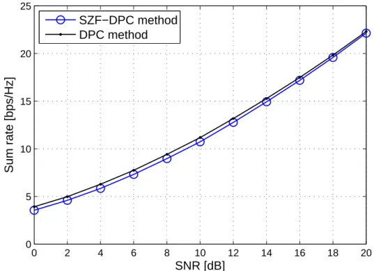
3.5 Comparison between the achievable sum rate of SZF-DPC method and the sum capacity, Nt= 4, Nr,k = 2, ∀k, and K = 2. . . 51
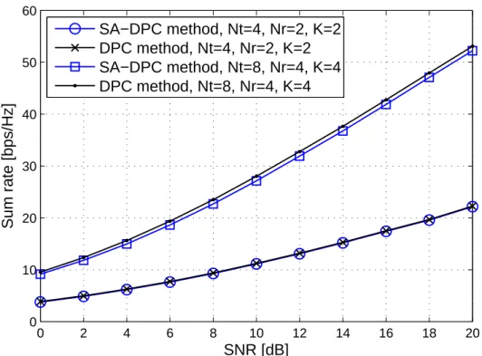
3.6 Comparison between the achievable sum rate of SA-DPC method and the sum capacity. . . 53
3.7 Interference removing techniques in non-linear methods . . . 54
3.8 Evolution of linear beamforming techniques . . . 55
3.9 Scheme of illustrating the noise enhancement problem problem. v1 has gain << 1 along h1 . . . 57
3.10 Comparison between the achievable sum rate of ZF method and sum capacity. . . 57
3.11 Comparison between the achievable sum rate of BD method and the sum capacity. . . 60
3.12 Comparison between the achievable sum rate of CB method and the sum capacity. . . 62
3.13 Comparison between the achievable sum rate of ZF-SA method and the sum capacity. . . 66
3.14 Comparison between the achievable sum rate of MMSE method and the sum capacity, . . . 70
3.15 Interference removing techniques in linear methods . . . 71
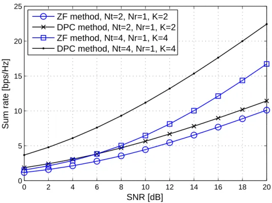
3.16 Sum rate comparison of ZF-DPC method, ZF method and the sum capacity. . . 72
3.17 Sum rate comparison of SZF-DPC method, BD method and the sum capacity. . . 73
3.18 Sum rate comparison of SA-DPC method, ZF-SA method and the sum capacity. . . 74
3.19 Sum rate comparison of SZF-DPC method, SA-DPC method, ZF-SA method, BD method, MMSE method and the sum capacity. . . 75
3.20 Sum rate comparison of DPC method, Per-OPT method, Nt = 4, Nr,k= 2, ∀k, and K = 2. . . 79 3.21 Sum rate comparison of DPC method, Per-OPT method, PBD-DPC
method, Nt = 4, Nr,k = 2, ∀k, and K = 2. . . 82 4.1 Sum rate comparison of DPC method and Prop-T method method,
Nt= 4, Nr,k = 2, ∀k, and K = 2. . . 87 4.2 Complexity comparison of SA-DPC and Prop-T methods. Nt= 4, and
Nr,k= 2, ∀k. . . 88 4.3 Sum rate comparison of DPC method, Per-OPT method, PBD-DPC
method, Prop-T method and Prop-P method, Nt = 8, Nr,k = 2, ∀k, K = 4, and Pn= PNTt. . . 92 4.4 Iteration number comparison of Per-OPT method and Prop-P method,
Nt= 8, Nr,k = 2, ∀k, and K = 4. . . 93 4.5 Processing time comparison of Per-OPT method and Prop-P method,
Nt= 8, Nr,k = 2, ∀k, and K = 4. . . 94 4.6 Sum rate comparison of DPC method, PBD-DPC method, Prop-T method,
and Prop-P method, Nt= 4, Nr,k= 2, ∀k, K = 2, and Pn= PNTt. . . . 95 4.7 Sum rate comparison of DPC method, PBD-DPC method, Prop-T method,
and Prop-P method, Nt= 4, Nr,k= 2, ∀k, K = 2, and Pn= PPNtT
l=1l
LIST OF FIGURES 15
4.8 Sum rate comparison of DPC method, Prop-T method, and Prop-P method, Nt= 4, Nr,k= 4, ∀k, K = 4, and Pn = PNTt. . . 97 4.9 Illustration of the power allocation over the transmit antennas under the
total power constraint and the per-antenna power constraint, Nt = 4, Nr,k = 4, ∀k, K = 4, PT = 1, and Pn = 0.25, ∀n. . . 98 5.1 The ratio of the processing time between GP method over the proposed
method. . . 105
5.2 Sum rate comparison of DPC method, GP method, and the proposed method. Nt= 8, Nr = 2, and K = 4. . . 106 5.3 Illustration of the sum rate approaching the sum capacity with power
List of Acronyms
MIMO Multiple-Input Multiple-Output BC Broadcast Channels
MAC Multiple Access Channels
Non-linear beamforming techniques
ZF-DPC Zero Forcing-Dirty Paper Coding
SZF-DPC Successive Zero Forcing-Dirty Paper Coding SA-DPC Successive Allocation-Dirty Paper Coding
Linear beamforming techniques
ZF Zero Forcing
BD Block Diagonalization CB Coordinated Beamforming
ZF-SA Zero Forcing-Successive Allocation MMSE Minimum Mean Square Error
Beamforming techniques under per-antenna power constraint
Per-OPT Per-Optimal
PBD-DPC Per Block Diagonalization-Dirty Paper Coding
1
Introduction
1.1
Background
With the emerging of the fourth generation (4G) wireless systems, commercial wireless communications such as mobile multimedia, mobile online game, and high quality video etc. come into our daily life. Meanwhile, the requirement for radio spec-trum also increases strongly with this fast development of wireless communication industry and business. The radio spectrum resource being limited, it becomes more and more expensive [37]. In order to meet the requirement of extremely high data rates, a large number of new techniques that can improve the spectrum efficiency and data rates are being studied, and tremendous research efforts are also undertaken to de-velop advanced coding, modulation, signal processing and multiple-access schemes for improving the quality and spectral efficiency of wireless links (e.g. FDMA, CDMA, OFDM, etc.). Multiple-Input Multiple-Output (MIMO) which transmits several dif-ferent data symbols at the same time and on the same frequency, is one key technique among them because of its ability to enhance the channel capacity of cellular systems at no extra cost of spectrum [1], [2]. MIMO technique is first investigated in point to point scenario, that is, the transmitter equipped with multiple transmit antennas and the receiver equipped with multiple receive antennas. The work in [3], [4] and [5] predicts that remarkable spectral efficiencies for wireless systems with multiple antennas can be obtained when the channel exhibits rich scattering. The work in [6] and [7] points
0 2 4 6 8 10 12 14 16 18 20 0 5 10 15 20 25 SNR [dB] Capacity [bps/Hz] Nt=1, Nr=1 Nt=2, Nr=1 Nt=2, Nr=2 Nt=4, Nr=4
Figure 1.1: Illustration of capacities with different antennas configurations. out that for an independent and identically distributed Gaussian noise channel, the ca-pacity of MIMO systems can grow linearly with the number of transmit or receive antennas. Figure 1.1 shows the different capacities with different antennas configura-tions over fading channel. When SNR is 10dB, the capacity for single transmit and receive antenna system is 3 bps/Hz, approximately. A two transmit antennas and one receive antenna system would achieve 4 bps/Hz. A four transmit antennas and four receive antennas system can reach 12 bps/Hz. In addition, the existing 802.11n [38] and 802.16e [39] standards also employ MIMO systems.
The benefits offered by MIMO systems are built on two underlying gains (i.e., spatial diversity and spatial multiplexing), which come with the increased cost of ra-dio frequency hardware. Compared with the conventional Single-Input Single-Output (SISO) systems, MIMO systems have more degrees of freedom regarding the signal transmission. Generally, there are three major transmission models in MIMO system: Diversity [40], Multiplexing [41], and Diversity mixed with Multiplexing [42].
1, MIMO Diversity
Wireless channels severely suffer from fading phenomena, which causes unrelia-bility in data decoding. Fundamentally, the spatial diversity scheme sends multiple
1.1. BACKGROUND 21 copies of the signal through multiple transmit antennas, so that the probability that all the signal components fade simultaneously is reduced. Therefore, the reliability of the data reception is enhanced and improved [43].
Receive diversity can be used in Single-Input Multiple-Output (SIMO) channels. The receive antennas receive the signal with independent fading. Then the receiver combines these signals so that the resulted signal exhibits considerably reduced fad-ing [44]. The receive diversity order is characterized by the number of independently fading branches, and the maximum receive diversity order is equal to the number of receive antennas in SIMO channels. The transmit diversity is applicable to Multiple-Input Single-Output (MISO) channels [8], [11]. The transmit diversity order corre-sponds to the number of independently fading paths that a symbol passes through. Therefore, the maximum transmit diversity order of MISO system is equal to the num-ber of transmit antennas. For a general MIMO system with Nr receive antennas and
Nttransmit antennas, the maximum diversity order that can be achieved is
D = Nr× Nt (1.1)
where the channel between each transmit-receive antenna pair is assumed to fade in-dependently.
2, MIMO Multiplexing
In spatial multiplexing, a high rate signal is split into multiple lower rate streams and each stream is transmitted from a different transmit antenna in the same frequency channel. [4] has shown that in the high SNR region, the capacity of a channel with independent and identically distributed (i.i.d.) Rayleigh fading between each transmit-receive antenna pair is given by
C(SN R) = min{Nr, Nt} log(SN R) + O(1) (1.2)
where SN R is the signal to noise ratio. The spatial multiplexing transmission offers a linear increase with the number of receive or transmit antennas in the transmission rate for the same bandwidth and with no additional power expenditure [10]. Compared with the spatial diversity transmission, the spatial multiplexing transmission aims to maxi-mize the system capacity. One typical spatial multiplexing transmission model is Bell Laboratory Layered Space-Time (BLAST) system [45]. The maximum multiplexing gain of BLAST system is
The spatial multiplexing configuration can also be applied in a multiuser system. Recently, an extension of MIMO named Multiuser MIMO (MU-MIMO) system attracts more attention compared with MIMO system since spatially distributed users with multiple antennas can be served at the same time by using spatial diversity, at the cost of some more signal processing [8], [9]. The base station communicates with the multiple users simultaneously in the same frequency channel by exploiting differ-ences in spatial signatures induced by spatially dispersed users, this technique is also known as space-division multiple access (SDMA) [10]. It is shown that similar capac-ity scaling to MIMO systems can be achieved by dirty paper coding (DPC) technique in MU-MIMO systems. Some advantage of MU-MIMO systems can be obtained with the aid of beamforming techniques. By beamforming we mean all methods applied at the transmitter that facilitate detection at the receiver [46]. Although beamforming is not a new concept and has been used in MIMO systems as well [11], it is optional and used only to improve the SNR at the receiver [12]. However, in order to fully exploit the increased performance of spatial multiplexing in MU-MIMO systems, beamform-ing techniques are essential to eliminate or minimize multiuser interference (MUI). Note that normally, beamforming techniques are performed with the help of the known downlink channel state information (CSI)1at the base station.
The downlink, from the base station with multiple antennas to multiple users with one or more antennas per user, is denoted as MU-MIMO broadcast channels. Consid-ering the optimal beamforming technique in terms of capacity for this system, duality between the downlink MU-MIMO broadcast channels and the uplink multiple access channels (MAC), where several transmitter send different symbols to one common receiver, has to be used. The optimal beamforming vectors are then obtained with an iterative and numerically complex process. To reduce the computational complex-ity, some suboptimal near capacity methods are proposed. For example, zero forcing beamforming, coordinated beamforming, and DPC combined with user scheduling and zero forcing beamforming methods. Currently, there are still some challenges and problems for MU-MIMO beamforming techniques [48].
1. The assumption that full CSI available at the transmit side is valid in Time Division Duplex (TDD) systems because the uplink and downlink share the same frequency band. For Frequency Division Duplex (FDD) systems, however, the CSI needs to be estimated at the receiver and fed back to the transmitter. With beamforming techniques employed at the transmit side, the required computational effort for each receiver can be reduced, and eventually the receiver structure can be simplified [47].
1.2. MOTIVATION AND METHODOLOGY 23
1.2
Motivation and methodology
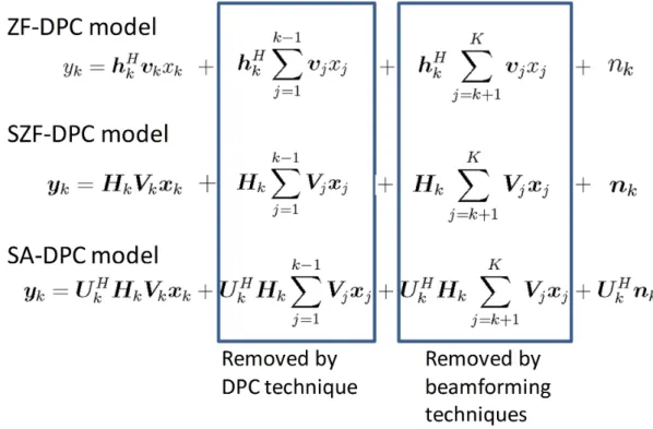
It is proven that DPC can achieve the sum capacity of the MU-MIMO broadcast channels [49], [13]. However, optimizing the transmit covariance matrix in DPC di-rectly is difficult because it is a non-concave optimization problem [13]. To avoid the complex processing, suboptimal solutions such as ZF-DPC method [14], SA-DPC method [15] and SBD-DPC method [16] are proposed, which divide the interference into two parts, one part is removed by DPC and the other part is suppressed by beam-forming techniques. ZF-DPC method only supports single receive antenna per user, and SBD-DPC method extends it to the multiple receive antenna per user case. SA-DPC method proposed in [15] finds the transmit beamforming and receive combining vectors of one data stream at each step for the user who can bring the largest through-put increase, the total number of receive antennas is further extended and can be larger than the number of transmit antennas. We denote these DPC involved beamforming techniques as non-linear methods. Even if the sum rates provided by these suboptimal non-linear methods are close to the sum capacity, obviously, the implementation of DPC increases the complexity of the transmitter and receiver design.
Therefore, linear processing solutions, such as ZF method [17], BD method [18], RBD method [4], CB method [19] and ZF-SA method [20] that eliminate the inter-ference completely by beamforming technique are considered. ZF and BD methods search for the transmit beamforming vectors of each user in the null space of the space spanned by other users. ZF-SA and CB methods adopt the receive combining tech-niques and extend the total number of receive antennas to be larger than that of trans-mit antennas. MMSE method proposed in [21] relaxes the zero-forcing condition, the transmit beamforming vectors are found by generalized eigenvalue technique. It can be seen that the sum rates offered by these methods are close to the sum capacity, and they are easy to implement, but these transmit beamforming vectors are designed under the assumption of a total power constraint.
In practice, the power amplifier of each antenna is limited individually by its linear-ity. Especially in an orthogonal frequency division multiplexing (OFDM) system, the peak-to-average power ratio (PAPR) is high [22]. Thus, a power constraint imposed on each transmit antenna is more realistic. Per-antenna power constraint beamform-ing techniques are studied in [23], [24], [25], [26] and [27]. [23] and [24] investigate the scenario where each user is equipped with a single antenna under the constraint of zero-forcing precoding. In [25], this constraint is relaxed and DPC technique is used to further improve the performance. In [26], authors analyze the case where each
user is equipped with multiple antennas via block diagonalization, and DPC is used under the assumption of a preset user order. However, the method in [26] assigns to a certain user a number of data streams depending on the rank of the relative channel matrix. This is suboptimal if, for instance, some of the subchannels are weak. In that case, the contribution of these subchannels to the sum rate might be negligible while they may impose severe constraints on the subchannels of subsequent users [15]. In [27], the optimal solution under per-antenna power constraint is exploited through the duality of MU-MIMO broadcast channels and corresponding uplink multiple access channels. Lagrange duality method and ellipsoid method are used to find the optimal value, which converge unfortunately quite slowly [25].
In this thesis, we propose a successive allocation of data streams to users. Mo-tivated by [15], one data stream is assigned at each step, the corresponding trans-mit beamforming and receive combining vectors are designed to maximize the global throughput. Moreover, a more practical per-antenna power constraint is imposed to the transmit antennas compared with [15], in which only a total transmit power constraint is considered. It is shown that the optimal solution in the original problem is difficult to obtain. In the proposed method, this problem is first divided into two classical opti-mization problems, which can be solved with existing standard algorithms. Then, we alternatively solve each subproblem under the assumption that the other is fixed sim-ilarly to [21]. The convergence can be achieved within a small number of iterations. At each step, the data stream is allocated to the user who brings the largest increase of the global throughput. The non-causally known interference is pre-subtracted through DPC technique before transmission, and the remaining interference is eliminated by the transmit beamforming and receive combining vectors. Note that the receive com-bining technique being adopted in the proposed method, the number of total receive antennas can be larger than that of transmit antennas.
In this thesis, we also propose an efficient power allocation method in multiuser MIMO broadcast channels. Since the original problem is non-deterministic polynomial-time (NP) hard when the interference is not removed completely, the optimal solution has extremely high computational complexity. Inspired by the classical water-filling algorithm, which assigns more power to the subchannels with large channel gains, we iteratively use water-filling algorithm to perform the power allocation. Simulation re-sults show that the performance is close to the optimal value, and the complexity is substantially reduced.
1.3. CONTRIBUTIONS 25
1.3
Contributions
The main contributions of this thesis are summarized as follows.
– An alternative approach to SA-DPC method is proposed. SA-DPC method cal-culates the transmit beamforming vector directly. In the proposed method, we first find the subspace where the transmit beamforming vector should lie in, then the one that maximizes the global throughput is selected. It is shown that the proposed method can be easily adapted to the scenario where the per-antenna power constraint is imposed.
– A new greedy data stream allocation method in multiuser MIMO broadcast chan-nels under the per-antenna power constraint is proposed. Since the spatial diver-sity in multiuser MIMO broadcast channels is fully exploited, compared with PBD-DPC method in [26], a better sum rate performance is achieved by the pro-posed method. In the propro-posed method, receive combining technique is adopted, and the data streams are assigned to users successively. The number of total re-ceive antennas may be larger than that of transmit antennas.
– An efficient power allocation method is proposed. Compared with the optimal solution, the proposed method has low computational complexity, and the per-formance is close to the optimum value.
1.4
Publications
– L. Zhao, Y. Wang, and P. Chargé. Zero-Forcing DPC Beamforming Design for Multiuser MIMO Broadcast Channels. Submitted to Signal Processing. Under review.
– L. Zhao, Y. Wang, and P. Chargé. Low Complexity Power Allocation in MU-MIMO Broadcast Channels. Submitted to International Journal of Electronics and Communications. Under review.
– L. Zhao, Y. Wang, and P. Chargé. Efficient Power Allocation Strategy in Mul-tiuser MIMO Broadcast Channels. PIMRC 2013.
– L. Zhao, Y. Wang, and P. Chargé. Efficient Iterative Water-filling Power Alloca-tion Method in MU-MIMO Broadcast Channels. MCC 2013.
– L. Zhao, Y. Wang, and P. Chargé. Joint Beamforming Design and Power Allo-cation for Multiuser MIMO Broadcast Channels. SIFWICT 2013.
– L. Zhao, P. Chargé, and Y. Wang. A Novel Zero-Forcing Transmit Data Scheme for Multiuser MIMO Broadcast Channels. SIFWICT 2013.
1.5
Outline of the thesis
The remainder of this thesis is organized into five chapters as listed below.
Chapter 2 introduces the structures of MIMO channel, MU-MIMO channel, and multiple access channels (MAC) channel. Brief capacity calculations of these channels are also given. MIMO channel is decomposed into several parallel SISO channels, and the well-known water-filling algorithm is used to perform the power allocation. For MU-MIMO channel, DPC technique is used to help to find the channel capacity.
Chapter 3 overviews the state of the art of beamforming techniques in the literature. Firstly, the non-linear methods taking advantage of DPC technique are discussed, then the linear beamforming methods are presented. After that, we consider the practical issues and address beamforming techniques under per-antenna power constraint. At last, the performance of these methods in terms of global throughput is compared, and we also give the advantages and disadvantages of each method.
Chapter 4 addresses the proposed beamforming methods. The first part introduces the proposed beamforming method under total power constraint, and the second part presents the proposed beamforming method under per-antenna power constraint. We also show the simulation results of each method, and give the performance compar-isons with other methods.
Chapter 5 introduces the proposed power allocation method when the interference is not completely removed. The original problem is a NP hard problem, and the optimal solution has very high computational complexity. Motivated by the classical water-filling algorithm, we propose a suboptimal method with a very low complexity. The performance is also quite close to the optimal value.
Chapter 6 gives the conclusions of this thesis and the possible directions in the future works.
2
Channel model
A signal propagating through a wireless channel arrives at the destination along a number of different paths, collectively referred to as multipath. These paths arise from scattering, reflection and diffraction of the radiated energy by objects in the environ-ment or refraction in the medium. The different propagation mechanisms influence path loss and fading models differently.
The signal power changes due to three effects : mean propagation (path) lose, macroscopic fading and microscopic fading. The mean propagation loss in macrocel-lular environment comes from inverse square law power loss, absorption by water and foliage and the effect of ground reflection. Mean propagation loss is range dependent. Macroscopic fading results from a blocking effect by buildings and natural features and is also known as long term fading or shadowing. Microscopic fading results from the constructive and destructive combination of multipaths and is also known as short term fading or fast fading. Multipath propagation results in the spreading of signal in different dimensions. There are delay spread, Doppler (or) frequency spread (Time-varying multipath channel) and angle spread. These spreads have significant effects on the signal. Mean path loss, macroscopic fading, microscopic fading, delay spread, Doppler spread and angle spread are the main channel effects. The details have been covered by a number of excellent papers and books [50], [51], [52], [53], [54]. They are beyond the scope of this dissertation. Our goal here is to optimize the capacity by using some well investigated propagation models.
2.1
MIMO channel model
We assume a complex baseband representation for the signal and channel unless otherwise specified. Consider a MIMO system with Nt transmit antennas and Nr
re-ceive antennas (Figure 2.1). The MIMO channel is given by the Nr×Ntmatrix H(τ, t)
with H(τ, t) = h1,1(τ, t) h1,2(τ, t) · · · h1,Nt(τ, t) h2,1(τ, t) h2,2(τ, t) · · · h2,Nt(τ, t) .. . ... . .. ... hNr,1(τ, t) hNr,2(τ, t) · · · hNr,Nt(τ, t) (2.1)
where hi,j(τ, t) is function of time, delay and amplitude gain between the jth transmit
antenna and the ith receive antenna. In [10], the elements of H are shown as indepen-dent zero mean circularly symmetric complex Gaussian random variables (Rayleigh random variables), with suitable choices of the scatterer location, antenna element pat-terns, and scattering model. Some properties of H are summarized below:
E{hi,j(τ, t)} = 0 (2.2)
E{|hi,j(τ, t)|2} = 1 (2.3)
E{hi,j(τ, t)hm,n(τ, t)∗} = 0 if i 6= m or j 6= n (2.4)
If the transmitted signal vector is s(t) ∈ CNt×1, then the received signal vector is
obtained as
y(t) = H(τ, t)s(t) + n(t) (2.5) where n(t) ∈ CNt×1is the Gaussian noise with independent and identically distributed
(i.i.d.) entries of zero mean and variance σ2. In the flat fading channel, since the output
at any instant of time is independent of inputs at previous times, the received signal can be expressed as
y = Hs + n (2.6)
2.2
MIMO capacity
We focus on the MIMO capacity in the frequency flat channel, the capacity in the frequency selectivity channel is not in the scope of this dissertation. First the channel
2.2. MIMO CAPACITY 29
Figure 2.1: Diagram of MIMO system.
H is supposed to be known at both the transmitter and receiver, the capacity of the MIMO channel is defined as [10]
C = max
f (s) I(s; y) (2.7)
where f (s) is the probability distribution of the vector s, and I(s; y) is the mutual information between vector s and y. Note that
I(s; y) = H(y) − H(y|s) (2.8) where H(y) is the differential entropy of the vector y, and H(y|s) is the conditional differential entropy of the vector y, given the knowledge of the vector s. Since the vector s and n are independent. i.e.,
H(y|s) = H(s + n|s) = H(n) (2.9) Then we have
I(s; y) = H(y) − H(n) (2.10) Maximizing the mutual information I(s; y) reduces to maximizing H(y). Note that the covariance matrix of y, Ryy = E[yyH] satisfies
Ryy = HRssHH + σ2INr (2.11)
where Rss is the covariance matrix of s. We know that amongst all vectors y with a
given covariance matrix Ryy, the differential entropy H(y) is maximized when y is
a zero mean circularly symmetric complex Gaussian vector [55]. This in turn implies that s must be a zero mean circularly symmetric complex Gaussian vector, and its
distribution is completely characterized by Rss. The differential entropies of vector y
and n are given by [10]
H(y) = log2|πeRyy| bps/Hz (2.12)
H(n) = log2|πeσ2I
Nr| bps/Hz (2.13)
therefore, I(s; y) reduces to [5]
I(s; y) = log2|INr +
1
σ2HRssH
H| (2.14)
and it follows from (2.7) that the capacity of the MIMO channel is given by C = max trace(Rss)=PT log2|INr + 1 σ2HRssH H| (2.15) where PT is the total transmit power. The capacity is often referred to as the error-free
spectral efficiency or the data rate per unit bandwidth that can be sustained reliably over the MIMO link.
In the above section, the properties of H are presented. Now, we study the capacity of a MIMO channel taking advantage of the properties of H. We assume that the CSI is perfectly known to both the receiver and the transmitter. The transmitter can benefit from this information in order to improve the MIMO channel capacity under the constraint of a fixed transmission power PT. By using the knowledge of the CSI,
the transmit power can be allocated in an optimal way on the transmit antennas. The idea behind this method, called water-filling, is to distribute more power to strong channels and less power to weak channels.
Consider a MIMO channel H with rank of r, through which a normalized signal vector x of dimension r is transmitted. Before transmission, the signal vector x is multiplied by the allocated power and the transmit beamforming matrix, i.e.,
s = V0√P x (2.16) where the unitary matrix V0is obtained from the singular value decomposition (SVD) of H (i.e., H = U0ΣV0H). √P is a diagonal matrix indicating the allocated power for the signal vector x. At the receiver, the received signal vector y is multiplied by
2.2. MIMO CAPACITY 31
Figure 2.2: Diagram of MIMO transmission.
Figure 2.3: Diagram of the decomposed parallel SISO channels.
the matrix U0H. The effective input-output relation for this system is given by y = U0HHV0√P x + U0Hn
= Σ√P x + ˜n (2.17) where ˜n is the r×1 transformed noise vector with covariance matrix E{ ˜n ˜nH} = σ2I
r.
Notice that Σ is a diagonal matrix containing the singular values of the channel matrix H. (2.17) shows that H can be explicitly decomposed (see Fig 2.3) into r parallel Single Input Single Output (SISO) channels satisfying
yi = λi
√
pixi + ˜ni, i = 1, 2, · · · , r. (2.18)
The capacity of the MIMO channel is the sum of individual parallel SISO channel capacities and is given by
C = r X i=1 log2(1 + λ 2 ipi σ2 ) (2.19)
Figure 2.4: Scheme of the Water-filling algorithm.
pi reflects the transmit power in the ith subchannel and satisfiesP pi = PT.
Since the transmitter can access the spatial subchannels, it can allocate variable power across the sub-channels to maximize the mutual information. The mutual infor-mation maximization problem now becomes
C = max P pi=PT r X i=1 log2(1 + λ 2 ipi σ2 ) (2.20)
The objective function for the maximization is concave with respect to the variables pi(i = 1, · · · , r) and can be maximized using Lagrangian method. The optimal power
allocation policy p? i, satisfies p?i = (µ −σ 2 λ2 i )+, i = 1, · · · , r (2.21) r X i=1 p?i = PT. (2.22)
where µ is a constant determined by the total transmission power and (a)+implies
(a)+= a if a ≥ 0 0 if a < 0 (2.23) This optimal power allocation solution is often referred as water-filling algorithm [56], which is pictorially described as Figure 2.4.
If the channel has no preferred direction and is completely unknown to the transmit-ter, the vector s may be chosen to be statistically non-preferential, i.e. Rss = PNTtINt.
anten-2.3. MU-MIMO CHANNEL MODEL 33 0 2 4 6 8 10 12 14 16 18 20 0 5 10 15 20 25 SNR [dB] Capacity [bps/Hz]
Unknown CSI at the transmitter Known CSI at the transmitter
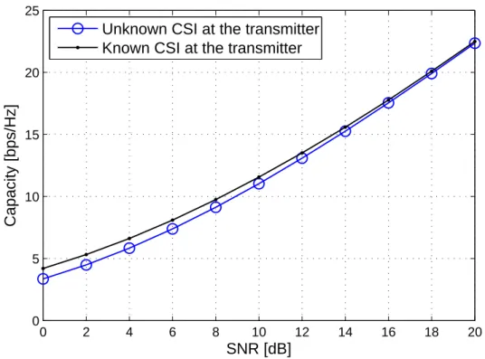
Figure 2.5: Comparison between the capacities of unknown CSI and known CSI at the transmitter, Nt= 4, Nr = 4.
nas. The capacity of the MIMO channel in the absence of channel knowledge at the transmitter is given by [10]
C = log2|INr +
PT
Ntσ2
HHH| (2.24) The capacity of the MIMO channel when channel is known to the transmitter is necessarily greater than that when the channel is unknown to the transmitter. This point can also be observed by the simulation results in Figure 2.5.
2.3
MU-MIMO channel model
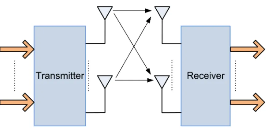
When a base station with multiple antennas supports multiple users with one or more antennas per user, we refer to this class of systems as multiuser MIMO (MU-MIMO). The downlink (forward link) from the base station to the users is a vector broadcast channel and the uplink (reverse link) is a vector multiple access channel. We focus on the downlink MU-MIMO broadcast channels, where a base station is equipped with Nt transmit antennas and serves K users, each user has Nr,k receive
Figure 2.6: Diagram of MU-MIMO system. antennas. The received signal yk ∈ CLk×1by the kth user is
yk = Hk K
X
j=1
Vjxj + nk (2.25)
where Lk is the number of data streams of the kth user; Hk ∈ CNr,k×Nt denotes
the channel between the transmitter and the kth user; xj ∈ CLj×1 is the transmit data
vector for the jth user; Vj ∈ CNt×Ljdenotes the transmit beamforming matrix, and the
allocated transmit power is included. Therefore, compared with (2.16), the transmitted signal can be represented as
s =
K
X
j=1
Vjxj (2.26)
Note that in downlink MU-MIMO broadcast channels, the transmit information for each user is emitted simultaneously, and each user can receive the information of all the users. Therefore, the transmit beamforming technique is essential for users to eliminate the interference, and enhance the desired information meanwhile.
2.4
MU-MIMO capacity
Before presenting the capacity calculation, we introduce dirty paper coding (DPC) first, which plays an important role for MU-MIMO capacity calculation.
2.4. MU-MIMO CAPACITY 35 interference known at the transmitter but unknown at the receiver is modeled as
Y = X + S + Z (2.27) where X and Y are the desired and received signals, respectively, S is the non-causally known interference, and Z is the unknown Gaussian noise. [57] shows that the capacity of this channel under the transmit power constraint is the same as if S did not exist. This technique is also referred to DPC technique.
Successive encoding of transmit information was proved to be optimum in terms of sum capacity in downlink MU-MIMO broadcast channels [14]. Given a preset user order in MU-MIMO broadcast channels, for the first encoded user, similarly to (2.25), the received signal can be written as
y1 = H1V1x1+ H1 K
X
j≥2
Vjxj+ n1 (2.28)
At the time of encoding the first user, signals from the following users are unknown, we receive it (i.e., H1PKj≥2Vjxj) with Gaussian noise together at the receiver.
For the kth (k ≥ 2) user encoding, the received signal can be written as yk= HkVkxk+ Hk k−1 X j<k Vjxj + Hk K X j>k Vjxj+ nk (2.29)
Note that at the time of encoding the kth user, the second term at the right hand of (2.29) (i.e., Hk
Pk−1
j<kVjxj) is known perfectly at the transmitter, which can be
regarded as non-existing by DPC technique. In this case, the data rate of the kth user is given by Rk = log2 |σ2I +PK j=kHkVjVjHHkH| |σ2I +PK j=k+1HkVjV H j HkH| (2.30)
Define the transmit covariance matrix as Qk = E[VkxkxkHVkH]. Note that the
sum capacity of MU-MIMO broadcast channels can be written as max {Qk}Kk=1 K X k=1 log2 |σ 2I +PK j=kHkQjH H k | |σ2I +PK j=k+1HkQjHkH| subject to K X k=1 trace(Qk) ≤ PT Qk≥ 0 (2.31)
(2.31) is neither a convex nor a concave problem. Direct optimization will gen-erally involve an exhaustive search over the entire space of covariance matrices that satisfy the power constraint and over the set of encoding orders, which is obviously very costly. Alternative methods to solve this problem have been proposed in [6], [49], [27], [58], [59], [60], [61], that exploit the relationship between the capacity region of the broadcast channels and that of its dual multiple access channels, which will be presented in the next chapter.
2.5
MAC model and capacity
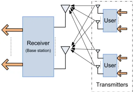
Given MU-MIMO broadcast channels as described in (2.25), the system model for the dual multiple access channels (MAC) (Figure 2.7) is
t = K X k=1 HkHUkxMk + n M (2.32)
where t ∈ CNt×1 is the received signal at the base station; HH
k ∈ CNt×Nr,k denotes
the channel between the kth user and the base station, notice that the channel matrix of MAC is the transpose conjugate of its dual broadcast channels; Uk is the transmit
beamforming matrix of the kth user. Define QMk = UkUkH as the transmit covariance
matrix of the kth user, and nM ∈ CNt×1is the Gaussian noise. Under a sum of transmit
power constraint, i.e.
K
X
k=1
trace(QMk ) ≤ PT (2.33)
it has been shown in [27] that the set of achievable rates in MAC by successively decoding users, which is optimum in terms of capacity, is equal to the set of achievable rates in the dual broadcast channels by performing a successive encoding of users. Moreover, given a set of covariance matrices and a particular decoding order, a method
2.5. MAC MODEL AND CAPACITY 37
Figure 2.7: Diagram of MAC system.
has been found to compute the covariance matrices that achieve the same rates in the broadcast channel by encoding users in reverse order, i.e., the user decoded first in the multiple access channel is encoded last in the broadcast channel. Note that MAC with constraint (2.33) is merely a mathematical tool that allows the computation of optimum operational points in broadcast channel. Obviously, a common power constraint shared by non-cooperating users lacks practical relevance.
As a consequence of these results, the maximization of (2.31) can be indirectly performed by first maximizing the sum of achievable rates in the dual MAC and then computing the covariance matrices that achieve that sum rate in the broadcast channels. Fortunately, the sum capacity optimization in MAC, given by
max {QM k }Kk=1 K X k=1 log2 |σ 2I +Pk j=1H H j QMj Hj| |σ2I +Pk−1 j=1H H j QMj Hj| subject to K X k=1 trace(QMk ) ≤ PT QMk ≥ 0 (2.34)
is a concave problem and therefore, can be maximized by using convex optimization techniques. Details will be given in the next chapter. In [27] it has been shown that the maximum value of (2.34) achieves the sum capacity of its dual MU-MIMO broadcast channels.
3
Beamforming techniques in
MU-MIMO broadcast channels
In the past decade, a great deal of research has been directed toward the devel-opment of transmit beamforming techniques for the downlink MU-MIMO broadcast channels (BC).
It is shown that the optimal transmit strategy given by information theory is DPC, which achieves the capacity region. Unfortunately, DPC does not directly lead to a realizable transmission strategy because of the coupled structure of the transmitted signals. The BC optimization problems are usually non-convex and thus cannot be solved directly. The key technique used to overcome this difficulty is to transform the non-convex BC problem into a convex MAC problem via so called BC-MAC duality relationship. However, the computational complexity of the sum capacity optimiza-tion is still significant. Consequently, there has been substantial interest in developing transmission strategies that approach the performance of optimal solution and are eas-ier to realize in practice.
Non-linear zero-forcing DPC techniques separate the interference into two parts, one part which is non-causally known at the base station can be removed by DPC technique and the rest part is eliminated by transmit beamforming vectors. Since these methods have quite low computational complexities, and their performances are close to the optimal solution, substantial research attentions have been observed in recent
years.
In addition, linear beamforming techniques that avoid the non-linear DPC-like pro-cessing is also promising since the structures of the transmitter and receiver are much more simple and easier to implement, such as zero-forcing (ZF), block diagonalization (BD), and coordinated beamforming (CB).
3.1
Optimal solution
As discussed in Chapter 2, owing to the special structure of the BC, the associated capacity region computation and beamforming optimization problems are typically non-convex, and thus cannot be solved directly. One feasible approach is to consider the respective dual MAC problems, which are easier to deal due to their convexity properties. In the literature, two different BC-MAC dualities are studied substantially. One is subject to a total transmit power constraint (denoted as conventional BC-MAC duality), and another one is based on minimax duality.
Conventional BC-MAC duality discussed in [6], [49], [13], [58], [62], [63], [28], [29] states that, under a single transmit total power constraint, the capacity region of the BC is identical to that of its dual MAC under the same total power constraint. The channel matrix associated with the dual MAC is the conjugate transposed channel matrix of the corresponding BC, and the noise covariance matrices of both the BC and its dual MAC are identity matrices.
The conventional BC-MAC duality is first observed by [62], and is applied to solve the sum power minimization problem for the BC with signal-to-interference-plus-noise ratio (SINR) constraint. Several methods are developed independently to prove the conventional BC-MAC duality. The proof in [62] is based on the equivalence between the optimal solutions of the power minimization problems for the BC and MAC with SINR constraint. [49] proves the conventional BC-MAC duality by presenting the explicit transformation between the transmit covariance matrix of the BC and that of the MAC, and applies this duality to solve the sum-capacity problem. The conventional BC-MAC duality is widely applied to solve a number of BC problems. [28] and [29] solve the SINR balance problem for the BC, by maximizing the minimal SINR problem among all the users under the total power constraint, and by transforming this problem into its dual MAC problem. The conventional BC-MAC duality is also used in [58] to show that DPC achieves the sum capacity. Moreover, the entire capacity region for the BC can be obtained using the conventional BC-MAC duality.
3.1. OPTIMAL SOLUTION 41 of linear power constraints, states that any boundary point of a BC capacity region can be obtained by solving a minimax optimization problem in its dual MAC. The channel matrix of the dual MAC is the conjugate transposed channel matrix of the corresponding BC, and the noise covariance matrix of the dual MAC is unknown for the minimization step of the minimax optimization problem.
Minimax duality proposed in [59], unifies the conventional BC-MAC duality. How-ever, only the sum capacity is considered in [59]. Furthermore, [64] extends minimax duality to solve the capacity region computation problem and beamforming optimiza-tion problem for the BC with a per-antenna power constraint. Using a minimax opti-mization approach, the sum capacity of the MIMO-BC is also studied in [60].
In [27], authors propose a general BC-MAC duality that combines the conventional BC-MAC duality and minimax duality. It can be applied to solve the capacity region computation of the BC under the total power constraint. In addition, the optimal rate region under per-antenna power constraint can also be obtained with multiple linear transmit covariance constraints. In the following, we focus on the case where a total power constraint is imposed to exploit the capacity region of the BC. The general BC-MAC duality compares the SINR of each data stream for both the primal BC and its dual MAC. At the BS of the auxiliary MAC, successive interference cancellation (SIC) is deployed to decode the information of each user [65]. For this dual MAC, the decoding order among the users as well as the data streams of each user is the reverse of the encoding order in the primal BC. Let SIN Ri,j and SIN RMi,j denote the SINR
of the (i, j)th data stream in BC and its dual MAC, respectively. According to DPC principle, encoded data streams have non-causal information about earlier encoded data streams, and thus the interference due to the earlier encoded data streams can be completely removed. Therefore, we have
SIN Ri,j = pi,j uH i,jHivi,j 2 PK k=i+1 PN l=1pk,l uH i,jHivk,l 2 +PN l=j+1pi,l uH i,jHivi,l 2 + σ2 (3.1) and SIN RMi,j = qi,j vi,jHHiHui,j 2 vH i,j( Pi−1 k=1 PN l=1qk,lHk Hu
k,luk,lHHk+Pj−1l=1 qi,lHiHui,lui,lHHi+ I)vi,j
(3.2)
where vi,j denotes both the transmit beamforming vector in the primal BC and the
both the transmit beamforming vector in the dual MAC and receive combining vector in the primal BC of the jth data stream of the ith user; pi,j and qi,j denote the transmit
power of the jth data stream of the ith user in the primal BC and the dual MAC, respectively; N is the number of data streams for each user.
The general BC-MAC duality states that : For a given primal MIMO BC with fixed transmit beamforming and receive combining vectors vi,j and ui,j, and fixed
transmit power pi,j for each data stream, which satisfy trace(
P
i,jpi,jvi,jvi,jH) = PT,
we can always find a set of transmit power qi,j for its dual MAC with fixed transmit
beamforming and receive combining vectors ui,j and vi,j, which satisfyPi,jσ2qi,j =
PT, such that the achievable SINR tuple of the primal BC is the same as that of its dual
MAC, i.e.,
SIN Ri,j = SIN RMi,j (3.3)
The proof is in Appendix A.
In the method proposed in [27], with a given user order, the received signal at the kth user is yk= HkVkxk+ Hk K X l>k Vlxl+ nk (3.4)
then the capacity optimization problem is written as max {Qk}Kk=1 K X k=1 log2 |σ 2I +PK j=kHkQjH H k | |σ2I +PK j=k+1HkQjHkH| subject to K X k=1 trace(Qk) ≤ PT Qk≥ 0 (3.5)
where Qj = VjVjH is the transmit covariance matrix. Unfortunately, as discussed
in Chapter 2, (3.5) is neither a convex nor a concave problem, direct optimization is difficult. According to the general BC-MAC duality, (3.5) can be transformed into a dual MAC problem as
max {QM k } K k=1 K X k=1 log2 |I + Pk j=1HjQ M j HjH| |I +Pk−1 j=1HjQMj HjH| subject to K X k=1 trace(σ2QMk ) ≤ PT QMk ≥ 0 (3.6)
3.1. OPTIMAL SOLUTION 43 where QMk indicates the transmit covariance matrix in the dual MAC. The general BC-MAC duality proved that (3.5) and (3.6) can achieve the same optimal value. From the proof of general BC-MAC duality in Appendix A, we can see that the SINR relation-ship between the BC and its dual MAC relies crucially on the reciprocity relationrelation-ship [5]. In [27], a MAC-BC covariance transformation algorithm between QMk and Qk
is proposed to find Qk when QMk is obtained (Algorithm 1). Note that the objective
function of (3.6) can be reordered as [66]
K X k=1 log2 |I + Pk j=1HjQMj HjH| |I +Pk−1 j=1HjQMj HjH| = K X k=1 log2|I + k X j=1 HjQMj H H j | − K X k=1 log2|I + k−1 X j=1 HjQMj H H j | = K−1 X k=1 log2|I + k X j=1 HjQMj H H j | + log2|I + K X j=1 HjQMj H H j | − K−1 X k=1 log2|I + k X j=1 HjQMj H H j | = log2|I + K X j=1 HjQMj HjH| (3.7)
Therefore, the problem (3.6) can be simplified as max {QM k } K k=1 log2|I + K X k=1 HkQMk H H k | subject to K X k=1 trace(σ2QMk ) ≤ PT QMk ≥ 0 (3.8)
This is a convex problem and the standard techniques (e.g. CVX, Yalmip) can be used to get the optimal transmit covariance matrix QMk ?. Then the BC transmit covariance matrix Qk is found by the MAC-BC covariance transformation algorithm.
Note that the decoding order of the BC is the reverse of the encoding order of its dual MAC.
The optimal solution can be found by this method. But in practice, suboptimal methods, that are much easier to implement with no significant performance degrada-tion, also attract substantial attentions. Next, we introduce several famous suboptimal
Algorithm 1 MAC-BC covariance transformation algorithm Input QMk , 1 ≤ k ≤ K
for k = 1 : K do
Compute the eigen value decomposition of QM k
?
= UkΛkUkH
for j = 1 : N do
Define uk,las the lth column of Uk
Define qk,l as the lth diagonal element of Λk
Obtain vk,jby MMSE receiver
vk,j = (
Pk−1 i=1
PN
l=1qi,lHiHui,lui,lHHi +
Pj−1
l=1 qk,lHkHuk,luk,lHHk +
I)−1HkHuk,j
Normalize vk,j
Compute pk,j using SINRk,j = SINRMk,j[27]
end for
Compute Qk=PNl=1pk,lvk,lvk,lH
end for
methods. The DPC involved method is denoted as non-linear method and otherwise it is denoted as linear method.
3.2
Non-linear beamforming techniques
The first non-linear beamforming technique is ZF-DPC method. In this method, the total number of receive antennas can not be larger than that of transmit antennas, and each user is supposed to have one receive antenna. Then, this method is extended to SZF-DPC method, in which each user can have multiple receive antennas, but the total number of receive antennas can not be larger than that of transmit antennas. Then, SZF-DPC method is extended to SA-DPC method, in which the total number of receive antennas may be larger than that of transmit antennas. In Figure 3.1, the evolution of these non-linear beamforming techniques is given.
3.2.1
Tomlinson Harashima Precoder
Non-linear methods separate the interference into two parts, one part is removed by zero-forcing technique, and the rest part which is non-causally known is eliminated by DPC techniques. A practical implementation of DPC technique is the pre-equalization Tomlinson Harashima Precoder (THP) technique, which is proposed in [67] and [68], aiming to pre-subtract the non-causally known interference at the transmitter. THP is initially proposed for single-input single-output channels in the presence of
inter-3.2. NON-LINEAR BEAMFORMING TECHNIQUES 45
Figure 3.1: Evolution of non-linear beamforming techniques
symbol interference (ISI), and it is extended to BC in [69]. Several different criteria are proposed using THP including zero-forcing (ZF) [69], minimum mean square error (MMSE) [70]. In [71], a robust THP is investigated with imperfect channel state infor-mation (CSI) at the transmitter. The main idea of THP is that, the non-causally known interference produced by the previous precoded symbols can be pre-canceled before transmission at the transmitter, and the modulo operation can be adopted to ensure that transmit power does not exceed the power constraint.
Now, we introduce the pre-equalization THP technique that pre-subtracts the non-causally known interference at the base station. Suppose a base station with Nt
trans-mit antennas transtrans-mits information to K users, each user is equipped with one single receive antenna, the received signal by the kth user is
yk= hHkvkxk+ hHk k−1 X j=1 vjxj+ hHk K X j=k+1 vjxj+ nk (1 ≤ k ≤ K) (3.9)
where vkis the transmit beamforming vector for the kth user. The transmit symbol xk
can be written as xk = ak− k−1 X j=1 bk,jxj (1 ≤ k ≤ K) (3.10)
Figure 3.2: Block diagram of the transmitter
Figure 3.3: Block diagram of the receiver where akis the information symbol and bk,j is defined as
bk,j = hHkvj √ pj hH kvk √ pk (3.11) Using (3.11) and (3.10) in (3.9), we have
yk = hHkvk √ pkak+ hHk K X j=k+1 vjxj+ nk (1 ≤ k ≤ K) (3.12)
Therefore, the non-causally known interference hH k
Pk−1
j=1vjxjcan be pre-subtracted
completely from the base station. In next sections, we will show how to suppress the residual interference hHk PK
j=k+1vjxj.
Define bk = [bk,1, · · · , bk,k−1, 0, · · · , 0]T andxek = [x1, · · · , xk−1, 0, · · · , 0]
T as a
measure of pre-subtracting the known interference term in (3.9), which is shown in Figure 3.2. The transmit symbol xk are successively generated from the information
symbols akin (3.10).
If the information symbol akis uniformly distributed in an M -ary QAM
constella-tion, then E{aaH} = I