Control of Hybrid Renewable Energy Power Plant for Autonomous Systems

HAL Id: tel-03119519

https://hal.univ-lorraine.fr/tel-03119519

Submitted on 24 Jan 2021

HAL is a multi-disciplinary open access

archive for the deposit and dissemination of sci-entific research documents, whether they are pub-lished or not. The documents may come from teaching and research institutions in France or abroad, or from public or private research centers.

L’archive ouverte pluridisciplinaire HAL, est destinée au dépôt et à la diffusion de documents scientifiques de niveau recherche, publiés ou non, émanant des établissements d’enseignement et de recherche français ou étrangers, des laboratoires publics ou privés.

Autonomous Systems

Phatiphat Thounthong

To cite this version:

Phatiphat Thounthong. Control of Hybrid Renewable Energy Power Plant for Autonomous Systems. Electric power. Université de Lorraine, 2020. �tel-03119519�

Université de Lorraine

ECOLE DOCTORALE "Informatique, Automatique, Electronique-Electrotechnique, Mathématiques"

N° attribué par la bibliothèque |_|_|_|_|_|_|_|_|_|_|

Mémoire

en vue d’obtenir

L’Habilitation à diriger des recherches

Spécialité : Génie Electrique

par

Phatiphat THOUNTHONG

Docteur, Génie Électrique de l’Institut National Polytechnique de Lorraine Soutenue publiquement le 1 décembre 2020

Control of Hybrid Renewable Energy Power Plant for Autonomous Systems

Membres du Jury : Président :

Christophe TURPIN Directeur de Recherche CNRS, LAPLACE, Toulouse

Rapporteurs :

Éric MONMASSON Professeur – Université de Cergy Pontoise Daniel HISSEL Professeur – Université de Franche-Comté

Manuela SECHILARIU Professeur – Université de Technologie de Compiègne

Examinateurs :

Betty LEMAIRE-SEMAIL Professeur – Université de Sciences et Technologies de Lille Bernard DAVAT Professeur – Université de Lorraine

Serge PIERFEDERICI Professeur – Université de Lorraine Babak NAHIDMOBARAKEH Professeur – Université de Lorraine

Invité :

Noureddine TAKORABET Professeur – Université de Lorraine

-i-Abstract (English)

This application to Habilitation to Advise Researches is prepared with the GREEN laboratory of the University of Lorraine. It is a synthesis of my research work and a vision of my future projects, mainly in the spirit of scientific collaboration of the RERC (Renewable Energy Research Center) of the King Mongkut's University of Technology North Bangkok and the GREEN Laboratory of the University of Lorraine.

This document composes of three main parts. Part I is a long curriculum vitae. In Part II, it is the synthesis research works that I have done after my PhD thesis. It composed of two main topics: 1) a study of DC/DC converter (interleaved converter, three-level converter) for FC, PV, Battery, and supercapacitor applications; 2) energy management for hybrid system (FC/SC, FC/Battery, etc…). For the control approach, a classic linear control and a nonlinear control based on differential flatness estimation have been studied and compared in hybrid energy source. Finally, in Part III, it is a research perspective, developed for the next years, and a short conclusion.

-ii-Abstract (Français)

Ce dossier d’Habilitation à Diriger des Recherches est préparé en collaboration avec le laboratoire GREEN de l’Université de Lorraine. Il constitue une synthèse de mes travaux de recherche et une vision sur mes projets à venir principalement dans un esprit de collaboration scientifique du RERC (Renewable Energy Research Center) du King Mongkut’s University of Technology North Bangkok et le Laboratoire GREEN de l’Université de Lorraine.

Ce document est composé de trois grandes parties. La première partie correspond à mon curriculum vitae détaillé. La seconde est la synthèse des travaux de recherche réalisés après mon doctorat ou je présente deux principaux axes à savoir un axe sur les convertisseurs DC/DC (interleaved converter, three-level converter) pour les applications Pile à Combustible, Panneaux Photovoltaïques, batteries et super-condensateurs et un axe sur la gestion d’énergie des systèmes hybrides (association Pile à combustible-supercondensateur, Pile à combustible-batteries, etc…). Quant aux stratégies de commande, des régulateurs linéaires conventionnels et non linéaires basés sur le concept de platitude des systèmes différentiels ont été étudiés et comparés pour des applications liées à la gestion d’énergie des sources hybrides d’énergie électrique. Finalement la troisième partie est consacrée aux perspectives pour les prochaines années et à une brève conclusion.

-iii-Table of Content

Abstract i

Table of Content iii

Part I. Curriculum Vitae (Dossier Scientifique) 1

Suppressed

Part II. Research Works (Mémoire d’HDR) 72

II.1 Introduction 72

II.2 Renewable Energy Sources and Storage Devices 78

II.2.1 Renewable Energy Source 78

II.2.1.1 Fuel Cell 78

A. Fuel Cell Principle 78

B. Fuel Cell System 83

C. Fuel Cell Characteristics 85

II.2.1.2 Photovoltaic 89

A. Photovoltaic Principle 89 B. Photovoltaic Characteristics 91

II.2.2 Energy Storage Devices 97

II.2.2.1 Battery 97

A. Battery Principle (lead-acid battery) 97 B. Battery Characteristics 100

II.2.2.2 Supercapacitor 102

A. Supercapacitor Principle 102 B. Supercapacitor Characteristics 105 C. Supercapacitor Versus Battery as an Energy Storage Device 114

II.3 Hybrid Power Source 116

II.3.1 Power Converter Structure 116

II.3.2 DC/DC Converter 125

II.3.2.1 Classic Converter 125

A. Non-reversible Converter 125

B. Reversible Converter 126

II.3.2.2 Parallel Interleaved Converter 126

II.3.2.3 Three Level Converter 142

II.3.3 Hybrid Power Plants 152

II.3.3.1 Fuel cell/battery hybrid power source 152

A. System Description 152

B. Energy Management 153

C. Performance Validation 153

D. Conclusion 161

II.3.3.2 Fuel cell/supercapacitor hybrid power source 161 A. Modeling of the Hybrid Power Source 162 B. Energy Management and Control Laws 163 C. Performance Validation 168

D. Conclusion 175

II.3.3.3 Fuel cell/battery/supercapacitor hybrid power source 177

A. System Description 177

B. Energy Management of Hybrid Power Source 178 C. Performance Validation 184

II.3.3.4 Photovoltaic/supercapacitor hybrid power source 190 A. Modeling of the Hybrid Power Source 190

B. Energy Management 190

C. Performance Validation 191

D. Conclusion 195

II.3.3.5 Fuel cell/photovoltaic/supercapacitor hybrid power source 198 A. Modeling of the Hybrid Power Source 198 B. Energy Management of Hybrid Power Source 198 C. Performance Validation 199

D. Conclusion 210

Part III. Perspective and Conclusion 211

III.1 Research Perspective 211

III.2 Conclusion 221

References 223

Appendix: Brief Differential Flatness Based Control 233 @@@ END @@@

-72-II.1 Introduction

Energy is important to everyone’s life. Among different types of energy, electric energy is one of the most essential that people need every day. Electricity can be generated in many ways from various energy sources. Electric power can be generated by conventional thermal power plants (using fossil fuels, or nuclear energy), hydropower stations, and other alternative power generating units (such as wind turbine generators, photovoltaic arrays, fuel cells, biomass power plants, geothermal power stations, etc.). Fossil fuels (including coal, oil and natural gas) and nuclear energy are not renewable, and their resources are limited. Currently, most of the energy demand in the world is met by fossil and nuclear power plants. A small part is drawn from renewable energy technologies such as wind, solar, fuel cell, biomass and geothermal energy [Raj08], [Too09]. Wind energy, solar energy and fuel cells have experienced a remarkably rapid growth in the past ten years [Agl09], [Ber09a], [Mil09] because they are pollution-free sources of power.

The cost of wind turbine, solar photovoltaic, and fuel cell electricity is still high [Moc09], [Pat09], [Sal09]. Nevertheless, with ongoing research, development and utilization of these technologies around the world, the costs of solar cells and fuel cell energy are expected to fall in the next few years. As for solar cell and fuel cell electricity producers, they now sell power freely to end-users through truly open access to the transmission lines. For this reason, they are likely to benefit as much as other producers of electricity. Another benefit in their favour is that the cost of renewable energy falls as technology advances, whereas the cost of electricity from conventional power plants rises with inflation. The difference in their trends indicates that wind, hydrogen, and solar power will be more advantageous in future. In the near future, the utility power system at a large scale will be supplied by renewable energy sources, i.e., hybrid energy systems, in order to increase their reliability and make them more effective for grid connected applications, as shown in Fig. II.1.1.

Additionally, they generate power near the load centres (called “autonomous system” or “grid independence”, which eliminates the need to run high-voltage transmission lines through rural and urban landscapes. However, there are still some severe concerns about several sources of renewable energy and their implementation, e.g.,

1) capital costs and

-73-The intermittency problem, for example, of solar energy is that solar panels cannot produce power steadily because their power production rates change with seasons, months, days, hours, etc. If there is no sunlight, no electricity will be produced from the photovoltaic (PV) cell [Kol09], [Sen09]. For fuel cell, when a large load is applied to the cells, the sudden increase in the current can cause the system to stall if the depleted oxygen or hydrogen cannot be replenished immediately and sufficiently. Cell starvation can lead to a system stall, permanent cell damage or reduced cell lifetime [Tan04], [Cor06], [Cor08]. To protect the fuel cells from overloading and starvation, especially during transient conditions, excessive oxygen and hydrogen can be supplied to the cells during the steady-state operation, which increases the reserve of available power in anticipation of a load increase. This strategy, however, is conservative and leads to increased parasitic losses, decreased air utilization and thereby compromised system performance. Therefore, the fuel cell power or current slope must be limited to prevent a fuel cell stack from experiencing the fuel starvation phenomenon and to optimize the system.

-74-Fig. II.1.2. Grid Independence: renewable energy hybrid power plant.

Therefore, in order to supply electric power to fluctuating loads with a renewable hybrid power system in autonomous system, an electric energy-storage system [a battery or/and a supercapacitor (SC)] is needed to compensate for the gap between the output from the renewable energy sources and the load, in addition to the collaborative load sharing among those energies [Kak09], [Rea09], [Tho08b], see Fig. II.1.2.

-75-Moreover, hydrogen as an energy storage media has the potential to address both daily and seasonal buffering requirements. Systems that employ an electrolyzer to convert excess electricity to hydrogen coupled with hydrogen storage and regeneration using a fuel cell can, in principle, provide power with zero (or near zero) emissions. Hydrogen production by solar energy or wind energy is a ‘renewable–regenerative system’ [Ber09a], and this process is known as the electrolysis process. The basic principle is the following: when the photovoltaic input power exceeds the load power demand, the system controller determines that the energy should be directed to hydrogen production. In this kind of operation, i.e., a solar based renewable–regenerative system, almost half of the solar input energy is directed to hydrogen production and converted with 60% energy efficiency.

Based on present storage device technology, battery design has to supply the trade-off between specific energy, specific power, and cycle life. The difficulty in obtaining high values of these three parameters has led to some suggestions that the energy-storage system of distributed generation systems should be a hybridization of an energy source and a power source [Coo09], [Tho09g]. The energy source, mainly fuel cells or/and solar cells in this document, has high specific energy, whereas the power source has high specific power. The power sources can be recharged from the main energy source(s) when there is less demand. The power source that has received wide attention is the supercapacitor (or ‘ultracapacitor’, or ‘electrochemical double-layer capacitor’) [Bau09], [Ber09b], [Sch09].

The enhancements in the performance of renewable energy source power systems that are gained by adding energy storage are all derived from the ability to shift the system output. Firming up the renewable system is accomplished by ensuring that energy is available when there is a demand for it rather than being limited by the availability of the renewable resource. As a result, the system output may need to be shifted to periods when the hydrogen and/or the sun, for example, are not available [Tho07]. Depending on the size and type of the energy-storage system and the load, it may be possible to provide all of the power needed to support the load. A much more common scenario is for the energy storage to simply provide enough power for applications, like peak shaving, without having full load support capability. The energy-storage system may also provide sufficient energy to ride out electric service interruptions that range from a few seconds to a few hours. This is especially important for service disruptions that occur when the renewable resource is not available.

-76-For FC vehicle applications, General Motors (GM; USA) became the first automaker to demonstrate a drivable FC vehicle named the Electrovan in 1966. There are many types of FCs characterized by their electrolytes. One of the most promising to be used in electric vehicle applications is the polymer electrolyte membrane FC (PEMFC) because of its relatively small size, light weight, and ease to build [Na07], [Per07]. Today, many automobile companies (such as GM, Renault, Opel, Suzuki, Toyota, Daihatsu, DaimlerChrysler, Ford, Mazda) have demonstrated the possibilities of using the PEMFC as a main source in electric vehicles called FC vehicles (FCVs). The concept of an FCV is depicted in Fig. II.1.3. For example, after a long history of FC research and development from 1964, GM unveiled an FCV powered by PEMFC (75 kW, 125–200 V, 200 cells) to drive a wheel motor (a permanent magnet synchronous: 60 kW, 305 Nm) with a driving range of 400 km in 2000. In the United States, in 2002, the Honda FCX was the first FC car to be certified for use by the general public, and so theoretically become publicly available. This four-seater city car has a top speed of 150 km/h and a range of 270 km. The hydrogen fuel is stored in a high pressure tank [Hoo03].

-77-In industry, United Technologies Corporation (UTC) FC (USA) is involved in the development of the FC systems for space and defense applications. UTC FC activity began in 1958 and led to the development of the first practical FC application used to generate electrical power and potable water for the Apollo space missions. In 1998, UTC FC delivered a 100-kW FC power plant, with 40% efficiency, to Nova Bus for installation in a 40-ft, hybrid drive electric bus under a DOE/Georgetown University contract [Var06].

GM is involved in the development of PEMFCs for stationary power and the more obvious automotive markets [Hel07]. In February 2004, they began the first phase of installation operations in Texas at Dow’s chemical manufacturing, the largest facility in the world. These FC systems are used to generate 35MWof electricity.

Axane (France) was created in 2001 and is working on PEM FC technology [Lec04]. It is positioning itself to the objective three markets that are likely to provide large commercial outlets in the short term: 1) portable multiapplication generators (500 W–10 kW), 2) stationary applications (more than 10 kW), 3) mobile applications for small hybrid vehicles (5 kW–20 kW).

In this HDR document in Part II, many structures of renewable hybrid power source are proposed for both grid independence and vehicle applications. The basic principles, characteristics, and working constraints of the FC, PV, battery, and supercapacitor are presented in Section 2. The power circuit structures, the power electronics topologies, energy management and innovative energy control law (based on linear system and nonlinear differential flatness approach) are presented in Section 3.

-78-II.2 Renewable Energy Sources and Storage Devices

II.2.1 Renewable Energy Source

II.2.1.1 Fuel Cell A. Fuel Cell Principle

An FC is a device that converts the chemical energy of a fuel directly to electrical energy. Its concept was proposed approximately 170 years ago when William Robert Grove conceived the first FC in 1839, which produced water and electricity by supplying hydrogen (H2) and oxygen (O2) into a sulfuric acid bath in the

presence of porous platinum electrodes [Tho08a], see Fig. II.2.1. The process by which this is done is very similar to the electrochemical process by which a battery generates power; at one electrode, a fuel such as hydrogen is

oxidized, and at the other electrode an oxidant such as oxygen is reduced. The reactions exchange ions through a solid or liquid electrolyte and electrons through an external circuit, as shown in Fig. II.2.2.

Fig. II.2.1. Fuel cell principle discovered by Sir William Grove.

Sir William Robert Grove (11 July

1811 – 1 August 1896) was a Welsh judge and physical scientist. He was a pioneer of fuel cell technology.

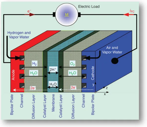
-79-Fig. II.2.2. Different layers of an elementary cell of PEMFC.

There are many different types of FCs, with the principal differences between them being the type of electrolyte and/or the type of fuel that they use. For instance, both the phosphoric acid FC (PAFC) and the molten carbonate FC (MCFC) have a liquid electrolyte, whereas a solid oxide FC (SOFC) has a solid, ceramic electrolyte [Cho06a], [Suz08], [Wan07a]. A proton exchange FC or polymer electrolyte membrane FC (PEMFC) and a direct methanol FC (DMFC) may have the same solid polymer electrolyte, but the DMFC uses liquid methanol for fuel whereas the PEMFC uses gaseous hydrogen [Ko08], [Paq08].

The PEMFC has many of the qualities required of an automotive power system including relatively low operating temperature, high power density, and rapid startup [Cor08], [Ema08], [Mit06]. In addition, PEMFC may also be used in residential and commercial power systems [Neh06].

-80-The FC model here is for a type of PEM, which uses the following electrochemical reaction:

Energy Electrical Heat+ + → + O H O 2 1 H_{2 2 2} . (2.1)

The theoretical value of a single cell voltage of FC is 1.23 V. It is never reached even at no load. At the rated current, the voltage of an elementary cell is about 0.6–0.7 V [Sad06], [Pag07], [Pas07]. Therefore, an FC is always an assembly of elementary cells that constitute a stack, as Fig. II.2.3 depicts. The examples of a FC stack are shown in Fig. II.2.3 to Fig. II.2.5 that have been used for studying in the following works both in the GREEN lab and the RERC lab.

In a single FC, the two plates [Fig. II.2.3(b)] are the last of the components making up the cell. The plates are made of a light weight, strong, gas-impermeable, electron-conducting material; graphite or metals are commonly used. The first task performed by each plate is to provide a gas flow field. The channels are used to carry the reactant gas from the point at which it enters the FC to the point at which the gas exits. Flow-field design also affects water supply to the membrane and water removal from the cathode. The second task served by each plate is that of current collector. With the addition of the flow fields and current collectors, the PEMFC is completed.

(a) (b)

Fig. II.2.3. PEMFC (23 cells, 500 W, 40 A, around 13 V), manufactured by the Centre for Solar Energy and Hydrogen Research Baden-Württemberg (ZSW) Company (Germany): (a) stack and (b) a serpentine flow field plate of 100 cm2. Pressed against the outer surface of each backing layer is a piece of hardware, called a plate, which often serves the dual role of flow field and current collector. It was functioned at the GREEN laboratory during 2002-2005.

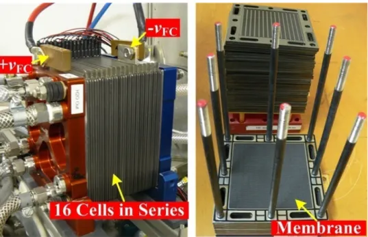
-81-Fig. II.2.4. PEMFC (16 cells, 500 W, 50 A, and around 11 V), manufactured by the Centre for Solar Energy and Hydrogen Research Baden-Württemberg (ZSW) Company (Germany). It is being functioned at the GREEN laboratory.

Fig. II.2.5. The Nexa PEMFC (1.2 kW, 46 A, around 26 V), developed and commercialized by the Ballard Power Systems Inc. It is being functioned at the RERC laboratory.

As developed earlier [Adz08], [Pas07], the Nernst equation for the hydrogen/oxygen FC, using literature values for the standard-state entropy change, can be written as

-82-(

)

( )

( )

where E is the reversible no-loss voltage of the FC (the thermodynamic potential), T is the cell temperature (K), pH2 and pO2 are the partial pressure of hydrogen and oxygen (bar), respectively,

and nCell is the number of cells in series.

The FC voltage VFC is modeled as [Adz08], [Pas07], [Sad06]

(

)

Activationloss _Ohmicloss Concentrationloss

i i I B i I R i i I A E V _      ₋ + ⋅ + + ⋅ −       + ⋅ − = L n FC n FC m O n FC FC log log 1 (2.3)

where IFC is the delivered FC current, iO is the exchange current, A is the slope of the Tafel line, iL is

the limiting current, B is the constant in the mass transfer term, in is the internal current, and Rm is

the membrane and contact resistances. These parameters can be determined from experiments. So, a typical fuel cell polarization characteristic with electrical voltage against current is shown in Fig. II.2.6.

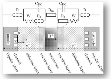
-83-Fig. II.2.7. Small signal equivalent electric circuit of the fuel cell.

Finally, Fig. II.2.7 shows an equivalent circuit valid for small signals [Fri04]. The electrodes are represented by a capacitor CDC which takes into account the double layer capacity appearing

because of an accumulation of electrons and protons on both sides of the reactive layer. The chemical reaction is represented by resistors Rt, diffusion effects by a Warburg impedance W, and

finally the membrane by an ohmic resistance Rm. The dashed parts of the circuit—electric resistance

of the bipolar plates and voltage drop of the anode—are neglected. By choosing a high frequency, the influence of the electrodes can be separated from the one of the membrane.

B. Fuel Cell System

Figure II.2.3 shows some of the tubes that deliver gases. There are usually 2 × 4 connections: two wires for the current, 2 × 2 tubes for the gases, and 1 × 2 tubes for the cooling system. As the gases are supplied in excess to ensure a good operation of the cell, the non consumed gases have to leave the FC carrying with them the produced water (Fig. II.2.8). Generally, a water circuit is used to impose the operating temperature of the FC (approximately 60–70 °C). At start up, the FC stack is warmed and later cooled at the rated current. Nearly, the same amount of energy generated is heat and electricity.

An FC stack requires fuel, oxidant, and coolant to operate. The pressure and flow rate of each of these streams must be regulated. The gases must be humidified, and the coolant temperature must be controlled. To achieve this, the FC stack must be surrounded by a fuel system, fuel delivery system, air system, stack cooling system, and humidification system.

-84-Once operating, the output power must be conditioned. Suitable alarms must shut down the process if unsafe operating conditions occur, and a cell-voltage monitoring system must monitor FC stack performance. These functions are performed by the electrical control systems.

Figure II.2.9 shows the simplified diagram of the PEMFC system of the stack presented in Fig. II.2.3. When an FC system is operated, its fuel flows are controlled by an FC controller that receives an FC current demand (reference), iFCREF, from the user (manual operation) or from the

energy-management controller (in case of automatic operation). The fuel flows must be adjusted to match the reactant delivery rate to the usage rate by the FC controller. For the FC system considered here, the FC current demand signal iFCREF is in a linear scale of 50 A/10 V.

Fig. II.2.8. External and internal connections of a PEMFC stack.

Fig. II.2.9. Simplified diagram of the PEMFC system. vFC, iFC, and iFCREF are the FC voltage, current, and current

-85-C. Fuel Cell Characteristics

Refer to (2.3) and Fig. II.2.6, the polarization curves of a selection of commercially available fuel cells (Fig. II.2.3) are shown in Fig. II.2.10, at pressures close to atmospheric. An FC power source is always connected to the dc bus by a DC/DC converter. Switching characteristics of the PEMFC (500 W, 40 A, refer to Fig. II.2.3) at steady-state when connecting with a boost converter are presented in Fig. II.2.11. It can be seen that the PEMFC contains a complex impedance component, which it is not purely resistive at a high switching frequency of 25 kHz [Tho06a], [Hin09]. One can observe that its output impedance depends on operating point. One can also see the nonlinearity of the FC voltage curve during the change of current slope from positive to negative or vice versa. It can be concluded that an FC model is composed of complicated impedances [Jun07], [Pag07].

Thounthong et al. [Tho07] (who worked with a 500-W PEMFC system by ZSW Company, Fig. II.2.3), Corrêa et al. [Cor04], [Cor05a] (who worked with a 500-W Ballard and 500- W Avista PEMFC system), and Zhu et al. [Zhu06] (who worked with a 500-W PEMFC system) have demonstrated that the electrical response time of an FC is generally fast, being mainly associated with the speed at which the chemical reaction is capable of restoring the charge that has been drained by the load. On the other hand, because an FC system is composed of many mechanical devices, the whole FC system has slow transient response and slow output power ramping [Jur05], [Wan07b].

-86-(a) (b)

Fig. II.2.11. Experimental Result: Switching characteristics of a 500 W PEMFC of 25 kHz at the FC current supply of (a) 10 A and (b) 40 A (rated current).

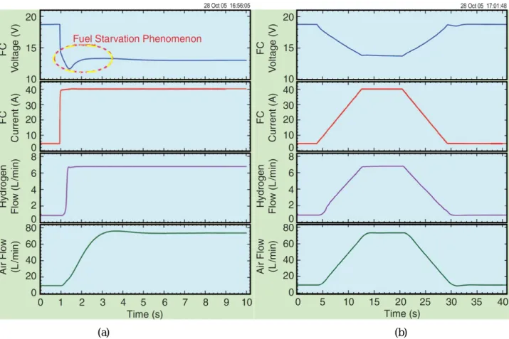
For clarity about the FC dynamics, Figure II.2.12 illustrates a ZSW PEMFC system (Fig. II.2.3), and it depicts the FC voltage response to a current demand of the PEMFC stack. The tests operate in two different ways: current step and controlled current slope of 4 A·s-1. One can scrutinize the voltage drop in Fig. II.2.12(a), compared to Fig. II.2.12(b), because fuel flows (particularly the delay of air flow) have difficulties following the current step. This characteristic is called fuel starvation phenomenon [Gay08], [Mei08], [Puk04], [Tho08a]. For the second test, Figure II.2.13 illustrates a Nexa PEMFC system (Fig. II.2.5), and it depicts the FC voltage response to a current demand of the PEMFC stack. One may see again the fuel starvation phenomenon. As illustrated in Fig. II.2.14, it also presents the worse case in which the FC system (Fig. II.2.3) shuts down because of a high FC-voltage drop from the fuel starvation problem. As already explained earlier, after the FC system is operated in many times of fuel starvation, its performance is reduced.

Reliability and lifetime are the most essential considerations in such power sources. Previous research, by Taniguchi et al. [Tan04], has clearly demonstrated that hydrogen and oxygen starvation caused severe and permanent damage to the electrocatalyst of the FC, as well as reducing its performance of voltage–current curve. They have recommended that fuel starvation must absolutely be avoided, even if the operation under fuel starvation is momentary, in just 1 s. As a result, to utilize the FC in dynamic applications, its current or power slope must be limited, for example, 4 A·s−1 for a PEMFC (0.5 kW, 12.5 V) [Tho06b]; a 2.5 kW·s−1 for a PEMFC (40 kW, 70 V) [Rod05]; and 500 W·s−1 for a PEMFC (2.5 kW, 22 V) [Cor05b].

-87-(a) (b)

Fig. II.2.12. Experimental Result: Dynamics characteristics of a 500 W ZSW PEMFC to (a) a high current step from 5 A to 40 A (rate current), (b) controlled current slope of 4 A·s-1_.

(a) (b)

Fig. II.2.13. Experimental Result: Dynamics characteristics of a 1.2 W Nexa PEMFC to (a) current step and (b) controlled current slope of 2 A·s-1_.

-88-Fig. II.2.14. FC starvation problem.

Remark 1: one may summarize the constraints to operate an FC as follows:

1) The FC power or current must be kept within an interval (rated value, minimum value or zero).

2) The FC current must be controlled as a unidirectional current.

3) The FC current slope must be limited to a maximum absolute value (for example, 4 A·s−1), to prevent an FC stack from the fuel starvation phenomenon.

4) Switching frequency of the FC current must be greater than 1.25 kHz, and the FC ripple current must be lower than around 5% of rated value, to ensure minor impact to the FC conditions [Cho04], [Gem03].

-89-II.2.1.2 Photovoltaic A. Photovoltaic Principle

Photovoltaic effect is a basic physical process through which solar energy is converted into electrical energy directly. The physics of a PV cell, or solar cell, is similar to the classical p-n junction diode, shown in Fig. II.2.15 [Wan06a]. A PV cell can basically be considered as a diode. When the cell is illuminated, the energy of photons is transferred to the semiconductor material, resulting in the creation of electron-hole pairs. The electric field created by the p-n junction causes the photon-generated electron-hole pairs to separate. The electrons are accelerated to n-region (N-type material), and the holes are dragged into p-region (P-type material),

shown in Fig. II.2.15. The electrons from n-region flow through the external circuit and provide the electrical power to the load at the same time. The PV cell shown in Fig. II.2.15 is the basic component of a PV energy system. Since a typical PV cell produces less than 2 W at approximately 0.5 V DC, it is necessary to connect PV cells in series-parallel configurations to produce desired power and voltage ratings. Figure II.2.16 shows how single PV cells are grouped to form modules and how modules are connected to build arrays. There is no fixed definition on the size of a module and neither for an array. A module may have a power output from a few watts to hundreds of watts. And the power rating of an array can vary from hundreds of watts to megawatts.

Fig. II.2.15. Schematic block diagram of a PV cell.

Alexandre-Edmond Becquerel (24

March 1820 – 11 May 1891) was a French physicist who studied the solar spectrum, magnetism, electricity and optics. He is credited with the discovery of the photovoltaic effect, the operating principle of the solar cell, in 1839.

-90-Fig. II.2.16. PV Cell, module, and array.

The most commonly used model for a PV cell is the one-diode equivalent circuit as shown in Fig. II.2.17. Since the shunt resistance Rsh is large, it normally can be neglected. The five

parameters model shown in Fig. II.2.17(a) can therefore be simplified into that shown in Fig. II.2.17(b). This simplified equivalent circuit model is commonly used in many studies [Wan04], [Amo00].

The relationship between the PV voltage VPV and the PV current IPV can be expressed as

[Xia06]:           − − = − =      + ⋅ 1 s PV PV O L D L PV κ R I V e I I I I I (2.4)

where IL = light current (A); IO = saturation current (A); IPV = PV current (A); VPV = PV output

voltage (V); Rs = series resistance (Ω); κ = thermal voltage timing completion factor (V). There are

four parameters (IL, IO, Rs and κ ) that need to be determined before the I-V relationship can be

obtained. That is why the model is called a four-parameter model. Both the equivalent circuit shown in Fig. II.2.17 and (2.4) look simple. However, the actual model is more complicated than it looks because the above four parameters are functions of temperature, load current and/or solar irradiance.

-91-(a) (b)

Fig. II.2.17. One-diode equivalent circuit model for a PV cell. (a) Five parameters model; (b) Simplified four parameters model.

B. Photovoltaic Characteristics

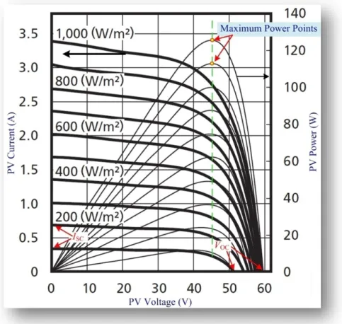
The model I-V and P-V characteristic curves under different irradiances are given in Fig. II.2.18 at 25 °C. It is noted from the figure that the higher is the irradiance, the larger are the short-circuit current (ISC) and the open-circuit voltage (VOC). And, obviously, the larger will be the

maximum power. The maximum power point (MPP), short-circuit current and open-circuit voltage are also illustrated in the figure.

The effect of the temperature on the PV model performance is illustrated in Fig. II.2.19. It is noted that the lower the temperature, the higher is the maximum power and the larger the open circuit voltage. On the other hand, a lower temperature gives a slightly lower short circuit current.

-92-Fig. II.2.18. Characteristic curves: current/power vs. voltage (cell temperature: 25 °C) of Sharp solar modules (Na-E125G5, 94.8 W) model under different irradiances.

Fig. II.2.19. I-V characteristic curves of the PV model [Kyocera PV Module (KC200GT, 142 W)] under different temperatures.

-93-Solar power source requires so much larger initial cost compared to conventional electricity generation techniques. Therefore, it is very natural to desire to draw as much power as possible from a PV array which has already been installed. Otherwise, the system would lose valuable solar energy. Maximum power output of the PV array changes when solar insolation, temperature, and (or) load levels vary. Control is, therefore, needed for the PV generator to always keep track of the maximum power points [Che10], [Gib10]. Trajectory of those maximum power points has been drawn in Fig. II.2.18. Maximum power point tracking (MPPT) is one of the techniques to obtain maximum power from a PV system.

Fig. II.2.20. Concept of MPP for PV system.

The problem considered by MPPT techniques is to automatically find the voltage VPVMPP or

current IPVMPP at which a PV array should operate to obtain the maximum power output PMPP under

a given temperature and irradiance. It is noted that under partial shading conditions, in some cases it is possible to have multiple local maxima, but overall there is still only one true MPP. Most techniques respond to changes in both irradiance and temperature, but some are specifically more useful if temperature is approximately constant. Most techniques would automatically respond to changes in the array due to aging, though some are open-loop and would require periodic fine-tuning. By controlling the switching scheme of the converter(s) connected to the PVs the maximum power points of the PV array can always be tracked, as shown in Fig. II.2.20.

-94-Several different MPPT techniques have been proposed in the literature. Two popular tracking methods based on power measurement are widely adopted in PV power systems: the perturbation and observation method (P&O, or “Hill climbing”) and the incremental conductance method (IncCond) [Xia06], [Esr07]. Actually, both P&O and IncCond are based on the same technique. Here, only a classic P&O technique is studied as following.

Fig. II.2.21. Divergence of hill climbing/P&O from MPP.

P&O involves a perturbation in the duty ratio of the power converter or a perturbation in the operating current of the PV array. In the case of a PV array connected to a power converter, perturbing the duty ratio or the PV array current and consequently perturbs the PV array voltage. From Fig. II.2.21, it can be seen in 4 cases:

I. Incrementing the current increases the power when operating on the left of the MPP, II. Decrementing the current decreases the power when operating on the left of the MPP,

-95-III. Incrementing the current decreases the power when operating on the right of the MPP, IV. Decrementing the current increases the power when operating on the right of the MPP,

Based on P&O MPPT, the algorithm for the PPVMPP is described in Fig. II.2.22, where the ∆I

defined PV current step size and ∆t the sampling time. Note that this sampling time must be higher

than a main program sampling time. Two sensors are usually required to measure the PV array

voltage and current from which power is computed. The process is repeated periodically until the MPP is reached. The system then oscillates about the MPP. The oscillation can be minimized by reducing the perturbation step size (∆I). However, a smaller perturbation size slows down the MPPT. A solution to this conflicting situation is to have a variable perturbation size that gets smaller towards the MPP [Esr07].

-96-Finally, to prove the implemented P&O for a PV panel, the PV (Ekarat Solar 800 W, 25 V) has been in installed on the roof of the laboratory building (KMUTNB, Thailand) and also used in the following work, see Fig. II.2.23. The P&O has been implemented in MATLAB/Simulink with a dSPACE controller. The ∆I is set at 0.1 A and ∆t is set at 6 ms. Fig.II.2.24 shows the experimental results of MPPT at t = 15:01:29 (estimate PPVMPP = 260 W) and at t = 09:30:17 (estimate PPVMPP =

300 W). One can see the excellent performance of the P&O algorithm.

Fig. II.2.23. PV panel (Ekarat Solar, 800 W) is installed on the roof of the laboratory building (KMUTNB, Thailand).

(a) (b)

-97-Remark 2: one may summarize the constraints to operate a PV system as follows:

PV power systems require some specific estimation algorithms to deliver the MPP. Because of the typical low-efficiency characteristics of PV panels, it is very important to deliver the maximum instantaneous power from these energy sources to the load. It is obligatory to use DC/DC or DC/AC converters with effective MPPT techniques.

II.2.2 Energy Storage Devices

II.2.2.1 Battery

A. Battery Principle (lead-acid battery)

Electrochemical batteries (or “batteries,”) are electrochemical devices that convert electrical energy into potential chemical energy during charging, and convert chemical energy into electric energy during discharging. A cell is an independent and complete unit that possesses all the electrochemical properties. Basically, a battery cell consists of three primary elements: two electrodes (positive and negative) immersed into an electrolyte as shown in Fig. II.2.25.

Because it is the most widespread battery

technology in today’s automotive and power system applications, the lead-acid battery case is used as an example to explain the operating principle theory of electrochemical batteries. A lead-acid battery uses an aqueous solution of sulfuric acid (2H+ + SO42−) as the electrolyte. The electrodes are

made of porous lead (Pb, anode, electrically negative) and porous lead oxide (PbO2, cathode,

electrically positive). The processes taking place during discharging are shown in Fig. II.2.26(a), where lead is consumed and lead sulfate is formed [Ro97], [Ehn09]. The chemical reaction on the anode can be written as

Pb+SO2₄− →PbSO₄ +2e− (2.5)

Gaston Planté (1834–1889) was the

French physicist who invented the lead-acid battery in 1859.

-98-This reaction releases two electrons and, thereby, gives rise to an excess negative charge on the electrode that is relieved by a flow of electrons through the external circuit to the positive (cathode) electrode. At the positive electrode, the lead of PbO2 is also converted to PbSO4 and, at

the same time, water is formed. The reaction can be expressed as

PbO₂ +4H+ +SO₄2−+2e− →PbSO₄+2H₂O (2.6) During charging, the reactions on the anode and cathode are reversed as shown in Fig. II.2.26(b) that can be expressed by:

Anode: PbSO₄+2e− →Pb+SO2₄− (2.7) And

cathode: PbSO₄ +2H₂O→PbO₂+4H+ +SO2₄− +2e− (2.8) The overall reaction in a lead-acid battery cell can be expressed as

overall: Pb+PbO₂+2H₂SO₄ ⇔2PbSO₄+2H₂O (2.9)

-99-(a) Discharging (b) Charging

Fig. II.2.26. Electrochemical processes during the discharge and charge of a lead-acid battery cell.

Fig. II.2.27. Lead-acid battery model.

The lead-acid battery has a cell voltage of about 2.03 V at standard condition, which is affected by the concentration of the electrolyte and the nominal discharge voltage level is 1.75V/cell, or approximately 87.5% of the nominal cell voltage rating. Then, the number of cells connected in series determines the nominal voltage of the battery system, and the capacity of the battery system is the basic factor in determining the discharge rate. The voltage is the force enforcing each of the electrons coming out of the battery and the capacity is the number of electrons that can be obtained from the battery. While the voltage is fixed by cell chemistry, the capacity is variable depending on the quantity of active materials.

-100-The equivalent circuit for a battery is shown in Fig. II.2.27. -100-The internal resistance is due to the resistance of electrolyte and electrode. Self-discharge resistance is a result of electrolysis of water at high voltages and slow leakage across the battery terminals at low voltages. The overvoltage is modeled as an RC circuit with a time constant in the order of minutes [Cas92], [Sal92].

B. Battery Characteristics

Battery manufacturers usually specify the battery with coulometric capacity (C, amp-hours), which is defined as the number of amp-hours gained when discharging the battery from a fully charged state until the terminal voltage drops to its cut-off voltage, as shown in Fig.II.2.28. It should be noted that the same battery usually has a different number of amp-hours at different discharging current rates. Generally, the capacity will become smaller with a large discharge current rate, as shown in Fig.II.2.29. Battery manufacturers usually specify a battery with a number of hours along with a current rate. For example, a battery labeled 100 Ah at C5 rate has a 100 amp-hour capacity at 5 amp-hours discharge rate (discharging current 100/5 = 20 A).

Another important parameter of a battery is the state-of-charge (SOC). SOC is defined as the ratio of the remaining capacity to the fully charged capacity. With this definition, a fully charged battery has an SOC of 100% and a fully discharged battery has an SOC of 0%. However, the term “fully discharged” sometimes causes confusion because of the different capacity at different discharge rates and different cut-off voltage (refer to Fig.II.2.28). The change in SOC in a time interval, dt, with discharging or charging current iBat may be expressed as

Bat Bat Q dt i SOC= ∆ (2.10)

where QBat is the rated capacity (Ah). For discharging, iBat is positive, and for charging, iBat is

negative. Thus, the SOC of the battery can be expressed as

( )

( )

-101-Fig. II.2.28. Cut-off voltage of a typical battery.

Fig. II.2.29. Discharge characteristics of a lead-acid battery.

Another important parameter of a battery is the state-of-health (SOH) of a battery is the percentage of its capacity available when fully charged relative to its rated capacity. For example, a battery rated at 30 Ah, but only capable of delivering 24 Ah when fully charged, will have a state-of-health of 24/30 × 100 = 80%. Thus, the state-state-of-health takes into account the loss of capacity as the battery ages.

Remark 3: one may summarize the constraints to operate a battery as follows:

1) A lower current charges the battery more uniformly. Also, excessive charging rates increase the chance of overheating, which can mean battery damage. Battery charging current may set at QBat/5 – QBat/10, in normal operation.

-102-2) Avoid over-discharge which leads to “sulfation” and the battery is ruined. The reaction becomes irreversible when the size of the lead-sulfate formations become too large.

3) Avoid overcharging causes other undesirable reactions to occur: Electrolysis of water and generation of hydrogen gas; electrolysis of other compounds in electrodes and electrolyte, which can generate poisonous gasses; bulging and deformation of cases of sealed batteries

II.2.2.2 Supercapacitor A. Supercapacitor Principle

Recent progress in supercapacitor technology has principally been applied in computer memory backup systems, but with the latest increases in capacitor energy storage levels, higher power applications [especially uninterruptible power supply (UPS) and hybrid vehicle] have become practicable. Electrochemical capacitors are presently called by a number of names: supercapacitor, ultracapacitor, or electrochemical double-layer capacitor. These terms are used interchangeably, and they refer to a capacitor that stores electrical energy in the interface that lies between solid electrodes and an electrolyte, as delineated in Fig. II.2.30 and Fig. II.2.31.

Hermann von Helmholtz (August 31,

1821 – September 8, 1894) was a German physician and physicist who made significant contributions to several widely varied areas of modern science.

-103-Fig. II.2.30. Principle of operation of a supercapacitor.

Fig. II.2.31. Construction details of supercapacitors with activated carbon electrodes.

The double-layer capacitor phenomenon was discovered by Helmholtz, one of the greatest natural scientists, who mathematically formulated the first main theorem of thermodynamics, in the 1800s. To maximize the capacitance C, the area A must be maximized and d minimized. Nowadays, the equivalent plate separation distance at the double layer consists of a few electrolyte molecule diameters of about 10−10 m. This plate separation distance is impossible in a conventional capacitor due to traditional dielectric breakdown, consisting of ionization followed by spark discharge. Terminal voltage of the supercapacitor is limited though, due to dissociation of the electrolyte. This

-104-limits the maximum voltage (2.5–3 V) of a supercapacitor cell used in this experiment to 2.5 V. Electrode area in the supercapacitor is maximized by use of activated carbon with an effective surface area up to 3,000 m2/g of material. The large surface area combined with the high capacitance per unit area yields the very large capacitance seen in the supercapacitor [Nel03].

Since the early 1990s, supercapacitors dedicated to high power industrial applications (capacitance up to some thousands farads, specific energy and specific power of several Wh/kg and kW/kg, respectively) have been available. The first high-power supercapacitors were developed by the Pinnacle Research Institute (PRI) for U.S. military applications such as laser weaponry and missile guidance systems. However, only in the 20th century did supercapacitors become well known in the context of hybrid electric vehicles promoted by the Department of Energy (DOE) under a supercapacitor development program. DOE supercapacitor development programs of long-term goals are specific energy >15 Wh/kg, specific power >2.0 kW/kg after 2003. Some example of recent supercapacitor technology can be seen in Fig.II.2.32-34.

-105-Fig. II.2.33. Maxwell supercapacitor cell and module studied in the RERC laboratory since 2007.

Fig. II.2.34. Maxwell supercapacitor bank (165 F, 48 V) studied in the RERC laboratory since August 2013.

B. Supercapacitor Characteristics

The supercapacitor model is very complex because of the distributed-parameter model. Many different models have been proposed for the double-layer effect [Nel03]. Recent works [Uzu08], [Nel03] have proposed that the reduced order model (as portrayed in Fig. II.2.35) for a supercapacitor cell is presented because of its simplicity and its operating times on the order of a few seconds. It is comprised of three ideal circuit elements: a capacitor CCell, a series resistor RS

called the equivalent series resistance (ESR), and a parallel resistor Rp. The parallel resistor Rp

models the leakage current found in all capacitors. This leakage current is equal to a few milliamps in a big supercapacitor.

-106-Fig. II.2.35. Simplified equivalent circuit of a supercapacitor cell including RP.

Many applications require the capacitors to be connected together, in series and/or parallel combinations, to form a “bank” with a specific voltage and capacitance rating. Normally, they are always connected in series. Capacitance variations affect the voltage distribution during cycling, and voltage distribution during sustained operation at a fixed voltage is influenced by leakage current variations. For this reason, an active voltage balancing circuit is employed to regulate the cell voltage.

It is common to choose a specific voltage, and thus, calculating the required capacitance. In analyzing any application, one first needs to determine the following system variables affecting the choice of supercapacitor:

1) maximum voltage, VSCMax;

2) working (nominal) voltage, VSCNom;

3) minimum allowable voltage, VSCMin;

4) current requirement, ISC , or the power requirement, PSC;

5) time of discharge, td;

6) capacitance per cell, CCell;

7) cell voltage, VCell.

Connecting many cells in series to form a bank, this does lead to an increase in total ESR and to a decrease in total capacitance. Defining nS as the number of capacitors connected in series, the

maximum capacitor voltage VSCMax, total ESR, and capacitance CSC of the capacitor bank can be

estimated as:

V_SCMax =n_S⋅V_Cell (2.12.1)

S Cell SC n C C = (2.12.3)

The discharge profile for a supercapacitor bank under a constant current is shown in Fig. II.2.36. A constant discharging current ISC is particularly useful when determining the parameters of

the supercapacitor. Nevertheless, Fig. II.2.36 should not be used to consider sizing supercapacitors for constant power applications such as a general power profile (drive cycle) used in electric vehicle. Worst case scenarios from drive cycle determine size of the storage devices. For example, Mitchell et al. [Mit06] presented that the Renault fuel cell automobile (SCENIC II, rated power of 70 kW of a PEMFC) needs a supplementary constant power (from battery) of around 30 kW for a 3 s for transient power (vehicle acceleration). Then, the discharge profile for a supercapacitor under a constant power PSC is shown in Fig. II.2.37.

Fig. II.2.36. Discharge profile for a supercapacitor under constant current.

-108-To estimate the minimum capacitance requirement CSCMin, one can write an energy equation

without losses (ESR neglected) under a discharging constant power PSC as:

C_SCMin

(

( )

)

1 _{− =}

(2.13)

Where vSC(t) is the supercapacitor terminal voltage. Then,

( )

Since the power being delivered is constant, the minimum voltage VSCMin and maximum

current ISCMax can be determined based on the current conducting capabilities of the supercapacitor.

Equations (2.13) and (2.14) can then be rewritten as:

SCMin SC 2 SCNom SCMin 2 C t P V V = − ⋅ d (2.15) SCMin SC 2 SCNom SC SCMax 2 C t P V P I d ⋅ − = (2.16)

The variables VSCMax and CSC are related by the number of cells in series. Voltage rating is

important, but the capacitor will also fail if the current is too high. The assumption is that the capacitors will never be charged above the combined maximum voltage rating of all the cells. Generally, VSCMin is chosen as VSCMax/2, from (2.13), resulting in the remaining energy of 25%.

In applications where high currents are drawn, the effect of the ESR has to be taken into account. The energy dissipated Eloss in the ESR, as well as in the cabling, connectors, and converter,

could result in an undersizing of the number of capacitors required. For this reason, one can theoretically calculate the losses in the ESR as:

= ∫d

( )

-109-To calculate the required capacitance CSC, one can rewrite (2.13) as:

_SCMin

(

)

2 1 E t P v V C − = _d + (2.18)

From (2.13) and (2.18), one obtains:

C_SC =

(

)

where χ is the defined energy ratio [Tho09b].

The SC bank is always connected to the dc bus by means of a two-quadrant dc/dc converter (bidirectional converter), as illustrated in Fig. II.2.38. Firstly, to demonstrate the high dynamics of supercapacitor source, Fig. II.2.40 presents the transient response of an SC converter interfacing between the dc bus and the SC bank (SAFT SC module: 292 F, 30 V, see Fig. II.2.39) [Tho09b]. The initial voltage of the SC bank is 30 V. It shows the SC current set-point (reference) iSCREF and

the measured SC current iSC. One can observe the high dynamic response of the supercapacitor

source from 0 to 50 A (discharging) in 0.4 ms. Unquestionably, the fast response of supercapacitor power source can function with the high inertia main source to improve the slow dynamics of the whole system. For the discharging characteristics of the SAFT SC module (292 F, 30 V), Fig. II.2.41 presents the transient response at a discharging constant current of 50 A. It shows the SC voltage vSC and the SC current iSC. Because of an aged supercapacitor bank, one can observe the

high voltage drop in ESR. One may verify the total capacitance CSC as:

F. v t I C SC 300 SC SC _∆ = ∆ ⋅ =

-110-Fig. II.2.38. Supercapacitor converter testing concept.

-111-Fig. II.2.40. Experimental Result: Supercapacitor dynamics response to a current step 0 A to 50 A of SAFT supercapacitor bank (292 F, 30 V).

Fig. II.2.41. Experimental Result: Discharge profile for a supercapacitor under a constant current of 50 A of SAFT supercapacitor bank (292 F, 30 V).

-112-For the next testing, Fig. II.2.42 presents the discharging characteristics of the Maxwell SC module (100 F, 32 V, see Fig. II.2.33) under a constant current of 50 A. It shows the SC voltage vSC

and the SC current iSC. One again may verify the total capacitance CSC as:

F. v t I C SC 105 SC SC _∆ = ∆ ⋅ =

Finally, Fig. II.2.43 presents the discharging characteristics of the Maxwell SC module (100 F, 32 V, see Fig. II.2.33) under a constant power of 400 W. It shows the SC power reference, the measured SC power, the SC voltage, and the SC current. One again may verify the total capacitance CSC as:

( )

Fig. II.2.42. Experimental Result: Discharge profile for a supercapacitor under a constant current of 50 A of Maxwell supercapacitor bank (100 F, 32 V).

-113-Fig. II.2.43. Experimental Result: Discharge profile for a supercapacitor under a constant power of 400 W of Maxwell supercapacitor bank (100 F, 32 V).

-114-C. Supercapacitor Versus Battery as an Energy Storage Device

The battery is still the most extensive energy storage device to provide and deliver electricity. Today, there are many kinds of battery technologies used, such as lead-acid, NiCd, NiMH, or Li ion. Using analytical expressions to model a battery behavior has always been limited by the complex nature of battery electrochemistry [Col07], [Lee08], [Szu08]. For lead-acid cell, the terminal voltage of battery VBat (see Fig. II.2.27) and internal resistance RBat are strong functions of

the SOC. The actual voltage curve is linear over most of its operating range; nevertheless, at the end of discharge, the voltage decreases very rapidly toward zero. This is because the internal resistance of a lead-acid battery is almost linear during discharge, but the losses are substantial below 25% SOC because of the increase in internal resistance of the battery. This is a reasonable work for the case of batteries used in electric vehicles, because the battery is typically operated only down to 60% SOC [or 40% depth of discharge (DOD), the amount of energy capacity that has been removed from a battery]. Usually, DOD is expressed as a percentage of the total battery capacity, and DOD = 100% − SOC.

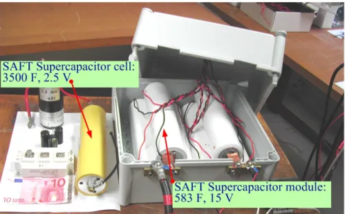
For the supercapacitor, an innovative prototype supercapacitor SC3500 model developed and manufactured by SAFT is 3,500 F, 2.5 V, 500 A, and 0.65 kg with a maximum energy storage capacity of 10,938 J (2 kW·kg-1 _{and 4:67 Wh·kg}-1_{) in an equivalent series resistance (ESR) of only}

0.8 mΩ (representing small losses). Terminal voltage of the supercapacitor is limited, though, because of dissociation of the electrolyte. This limits the maximum voltage of 2.5–3 V.

When comparing the power characteristics of supercapacitors and batteries, the comparisons should be made for the same charge/discharge efficiency. Only one half of the energy at the peak power from the battery is in the form of electrical energy to the load, and the other one half is dissipated within the battery as heat in the ESR. This is to say that the efficiency of batteries is around 50%. For supercapacitors, the peak power is usually for a 95% efficient discharge, in which only 5% of the energy from the device is dissipated as heat in the ESR. For a corresponding high-efficiency discharge, batteries would have a much lower power capability.

Furthermore, the main drawback of the batteries is a slow-charging time, limited by a charging current [Yan07]; in contrast, the supercapacitors may be charged/discharge in a short time depending on a high-charging current (power) available from the main source (see Fig. II.2.40 − Fig. II.2.43). The capacitor voltage vSC can then be found using the following classical equation:

( ) ( ) _SC( _o) o SC SC SC 1 t v d i C t v t t + ∫ = τ τ (2.20)

where iSC is the capacitor charging current.

Moreover, Fig. II.2.44 compares the advanced technologies of batteries and supercapacitors in terms of specific power and energy. Even though it is true that a battery has the largest energy density (meaning more energy is stored per weight than other technologies), it is important to consider the availability of that energy. This is the traditional advantage of capacitors. With a time constant of less than 0.1 s, energy can be taken from a capacitor at a very high rate [Oru07], [Uzu08], [Wan07c]. On the contrary, the same-size battery will not be able to supply the necessary energy in the same time. More advantageous, unlike batteries, supercapacitors can withstand a very large number of charge/discharge cycles without degradation (or visually infinite cycles) [Tho08a].

Fig. II.2.44. Specific power versus specific energy of modern storage devices: supercapacitor, lead-acid, and Li-ion battery technology. The supercapacitors and Li-ion batteries are based on the SAFT company.

Remark 4: one may summarize the constraints to operate a supercapacitor bank as follows:

To operate the SC module, its module voltage is limited to an interval [VSCMin,

VSCMax]. The higher VSCMax value of this interval corresponds to the rated

voltage of the storage device. In general, the lower VSCMin value is chosen as

VSCMax/2, where the remaining energy in the SC bank is only 25% and the SC

-116-II.3 Hybrid Power Source

II.3.1 Power Converter Structure

Solar and wind power generation are two of the most promising renewable power generation technologies. Fuel cells also demonstrate large prospective to be clean power sources of the near future because of many merits they have and the fast development in FC technologies. However, none of these technologies is perfect now. Solar and wind power are highly dependent on climate while fuel cells need hydrogen-rich fuel and the cost for fuel cells is still very high at current stage. Nevertheless, because different renewable energy sources can complement each other, multi-source hybrid alternative energy systems (with proper control) have great potential to provide higher quality and more reliable power to customers than a system based on a single resource.

There are many combinations of different alternative energy sources (photovoltaic and/or wind and/or fuel cell) and storage devices (battery and/or supercapacitor) to form a hybrid system. The solutions can be generally classified into two categories: AC coupling and DC coupling.

In an AC coupling scheme, shown in Fig. II.3.1, different energy sources are integrated through proper power electronic interfacing circuits to a power frequency AC bus. Coupling inductors may also be needed to achieve desired power flow management. The advantages of this coupling are as follows:

1) High reliability. If one of the energy sources is out of service, it can be isolated from the system easily.

2) Ready for grid connection.

3) Standard interfacing and modular structure. 4) Easy multi-voltage and multi-terminal matching. However, this structure has some disadvantages:

1) Synchronism required.

-117-Fig. II.3.1. Hybrid energy system integration: AC coupling.

In a DC coupling configuration, shown in Fig. II.3.2, different alternative energy sources are connected to a DC bus through appropriate power electronic interfacing circuits. Then the DC energy is converted into 50 Hz (France, Thailand, for example) or 60 Hz (USA) AC through a DC/AC converter (inverter) which can be bi-directional. For the DC link voltage level, it is depending on its applications:

■ 270 V or 350 V for the standard on the all-electric aircraft [Dol06]

■ 48 V [Agb04], 120 V [Wai05], or 400–480 V [Lee06], [Wan06b], [Cho06b] for stand-alone or parallel grid connections

■ 42 V (PowerNet) a new standard voltage for automobile systems [Ema08], [Fah04], [Kei04] ■ 270–540 V for electric vehicles [Luk08], [Gok02], [Bit04]

■ 350 V (transit bus systems) to 750 V (tramway and locomotive systems) [Var06], [Fur06], [Mon03], [Kim08], [Mil06], [Mil07], [Yon07], [Oga07], [Nic03].

-118-The advantages of the DC coupling are as follows:

1) Synchronism not needed for DC connection.

2) Suitable for long distance transmission; it has less transmission losses. 3) Single-wired connection

However, this structure has some disadvantages:

1) Concerns on the DC voltage compatibility

2) If the DC/AC inverter is out of service, the whole system fails to supply AC power.

Fig. II.3.2. Hybrid energy system integration: DC coupling.

A hybrid energy system can either be stand-alone (autonomous) or grid-connected if utility grid is available. For an autonomous application, the system needs to have sufficient storage capacity to handle the power variations from the alternative energy sources involved. A system of this type can be considered as a micro-grid, which has its own generation sources and loads. For a grid-connected application, the alternative energy sources in the micro-grid can supply power both to the local loads and the utility grid. In addition to real power, these sources can also be used to give reactive power support to the utility grid. The capacity of the storage device for these systems

-119-can be smaller if they are grid-connected since the grid -119-can be used as system backup. However, when connected to a utility grid, important operation and performance requirements, such as voltage, frequency and harmonic regulations, are imposed on the system.

However, here the stand-alone (autonomous) applications both FC vehicles and the renewable energy power plant with the DC coupling will be presented as following. Firstly, to control the power or current from the main energy source(s), a nonreversible DC/DC converter is always chosen to interface a main source to a DC bus. Then, we propose 7-configurations for the power converter connections.

• For the first one as detailed in Fig. II.3.3, it is very simple one that a main energy source S1 is connected to a DC bus by a DC/DC converter and an energy storage device E1 is directly connected to a DC bus [Tho08b]. An energy storage device should be a battery bank because battery voltage, for example, in a lead-acid battery, is nearly constant and virtually independent from discharge current and drops sharply when almost fully discharged. The main advantage is that it is no need a reversible DC/DC converter for an energy storage device E1. However, a battery bank should be composed of many cells connected in series in order to increase the utilized DC bus voltage.

• For the second one as presented in Fig. II.3.4, it is common configuration that a main energy source S1 is connected to a DC bus by a nonreversible DC/DC converter and an energy storage device E1 is connected to a DC bus by a reversible DC/DC converter [Tho07], [Tho11b]. An energy storage device can be either a battery bank or supercapacitor module. The main advantage of this configuration is that one can fully control a power from a main source and an energy storage device.

• For the third configuration as presented in Fig. II.3.5, a main energy source S1 is connected to a DC bus by a reversible DC/DC converter and an energy storage device E1 is connected to a terminal of a main source by a reversible DC/DC converter [Pay11]. An energy storage device can be either a battery bank or supercapacitor module. The main advantage of this configuration again is that one can fully control a power from a main source and an energy storage device. An