Les methodes numeriques pour les equations aux derivees partielles avec des conditions aux limites non locales

(1)

REPUBLIQUE ALGERIENNE DEMOCRATIQUE ET POUPU-LAIRE

MINISTERE DE L’ENSEIGNEMENT SUPERIEUR ET DE LA RECHERCHE SCIENTIFIQUE UNIVERSITE MENTOURI CONSTANTINE

FACULTE DES SCIENCES EXACTES

N d’ordre: N Série:

THESE

Pour obtenir le grade de

DOCTEUR D’ETAT EN MATHEMATIQUES Option:Analyse Numerique

LES METHODES NUMERIQUES POUR LES EQUATIONS AUX DERIVEES PARTIELLES AVEC DES CONDITIONS AUX LIMITES

NON LOCALES

Présentée par

AHMED CHENIGUEL

Le 14/05/2012

JURY

Président A.L. Marhoun Prof Université Mentouri Constantine

Rapporteur A. Ayadi Prof Université Elarbi Ben Mhidi-Oum Elbouaghi Examinateurs M. Bouzit M.C Université Elarbi Ben Mhidi-Oum Elbouaghi

... A.Hameida M.C Université Mentouri Constantine

...M.Reghioua M.C Ecole Normale Superieure de Constan-tine ...M.Djabbarni M.C Université Elarbi Ben Mhidi-Oum El- bouaghi

(2)

REMERCIEMENTS

Cette thèse est le fruit réalisé sous la direction du monsieur le pro-fesseur A. Ayadi, que je tiens particulièrement a remercier pour son encadrement et pour ces conseils qui ont été pour moi un appui con-sntant.

Je témoigne ma profonde reconnaissance a monsieur le professeur M.A.L. Marhoune qui malgré ces multiples taches a accepté la prési-dence de cette thèse. Je remercie aussi le Dr.M. Reghioua Maitre de conférence à l’école supérieure de Constantine qui malgré ces lourde taches de directeur de l’école normale supérieure de Constantine a ac-cepté de faire partie du jury d’examen de cette thèse. Je tiens a re-mercier le Dr M. Bouzit Maitre de conférence à l’université Elarbi Ben Mhidi qui s’est montré toujours très disponible durant l’achèvement de cette thèse. Je tiens aussi a remercier le Dr. A. Hameida Maitre de conférence à l’université Mentouri pour avoire accepté de faire partie du jury. Je tiens a remercier le Dr. M. Djabbarni Maitre de conférence à l’université Elarbi Ben Mhidi pour avoire accepté de faire partie du jury, je tiens a remrcier le Pr.K. Belarbi Professeur a l’institut d’électronique université Mentouri ainsi que le Dr;A. Lanani Maitre de conférence à l’université Mentouri pour leur encouragement durant la réalisation de cette thèse. Mon dernier remerciement va a monsieur le chef de départe-ment de mathématiques à l’université Mentouri le Dr. F. Rahmani pour son abnégation.

(3)

Contents

Introduction 4

1 An overview 11

1:1 High order compact f inite dif f erence 11

1.2 Consistency, Stability and Convergence 13

. 1.3 The compact scheme 17

1.4 Interior scheme 20

1.5 Adomian decomposition method 23

1.6 The Homotopy perturbation method 27

2-One dimensional di¤usion equation with an integral boundary con-dition

2.1 Sixth-order compact …nite di¤erence scheme 31

2.2 Standard Compact …nite di¤erence 31

2.3 Computational results 33

2.4 One dimensional nonhomogenous heat equation with nonlocal

boundary conditions 36

2.6 Numerical examples 38

2.7 Conclusion 45

2.8 One-dimensional nonhomogeneous di¤usion equation withe deriv-ative boundary conditions..58

2.11 Conclusion 64

2.12 A two-dimensional di¤usion equation 81

2.15 A three-dimensional di¤usion equation 96

3 Numerical method for solving wave equation with an integral bound-ary condition

3.3 Conclusion 115

3.4 The homotopy perturbation method for solving nonlocal

prob-lems 122

3.5 Analysis of the homotopy perturbation method 123

(4)

Liste of Tables

Absolute error for various spatial lenghts: 2.1 Absolute error for hx = 0:125 and ht= 0:001.

2.2 Absolute error for..hx= 0:1 ::: == ht = 0:001:::::::: :::::::::::::::::::::::::::::::::::::::::::::::::::::::::::::

2.3 Absolute error for..hx= 0:1. and ht = 0:01:::::::::: ::::::::::::::::::::::::::::::::::::::::::::::::::::::::::::

2.4 Absolute error for..hx= 0:1....and.ht= 0:01:::::::::::::::::::::::::::::::::::::::::::::::::::::::::::::::::::::::

2.5 Absolute error for. hx= 0:1...and:ht= 0:25:::::::::::::::::::::::::::::::::::::::::::::::::::::::::::::::::::::::

2.6 Absolute error for. hx= 0:1:::and ht = 0:25::::::::::::::::::::::::::::::::::::::::::::::::::::::::::::::::::::::

2.7 Absolute error for..hx= 0:1...and ht= 0:25:::::::::::::::::::::::::::::::::::::::::::::::::::::::::::::::::::::::

2.8 Absolute error for .hx= 0:1...and ht= 0:25::::::::::::::::::::::::::::::::::::::::::::::::::::::::::::::::::::::

2.9 Absolute error for..hx= 0:1:::::and ht= 0:01::::::::::::::::::::::::::::::::::::::::::::::::::::::::::::::::::::::

2.10 Absolute error forhx= 0:1:::::and ht= 0:0250:::::::::::::::::::::::::::::::::::::::::::::::::::::::::::::::::::

2.11 Absolute error for hx = 0:1:::::and ht= 0:0250:::::::::::::::::::::::::::::::::::::::::::::::::::::::::::::::::::

2.12 Absolute error for hx = hy = 0:1and ht= 0:0250:::::::::::::::::::::::::::::::::::::::::::::::::::::::::::::::::::::::::::::::::::::::::

2.13 Absolute error for hx = hy = hz = 0:1and ht= 0:0250:::::::::::::::::::::::::::::::::::::::::::::::::::::::::::::::::::::::::::::::::::

2.14 Absolute error for hx = hy = hz = 0:1...and ht =

0:0250:::::::::::::::::::::::::::::::::::::::::::::::::::::::::::::::::::::::::::

3.1 Absolute error for hx = 0:1and ht= 0:0250:::::::::::::::::::::::::::::::::::::::::::::::::::::::::::::::::::::::::::::::::::::::::::::::

3.2 Absolute error for hx = 0:1and ht= 0:0250::::::::::::::::::::::::::::::::::::::::::::::::::::::::::::::::::::::::::::::::::::::::::::::

3.5 Absolute error for hx = 0:1 and ht= 0:0250::::::::::::::::::::::::::::::::::::::::::::::::::::::::::::::::::::::::::::::::::::::::::::::

(5)

Liste of …gures 2:1 f or example (2:1) 2:2 f or example (3; 1) 2:3 f or example (3; 3) 2:4 f or example (3; 3) 2:5 f or example (4) 2:6 f or example (4) 2:7 f or example (5) 2:8 f or example (5) 2:9 f or example (1) 2:10 f or example (1) 2:11 f or example (1) 2:12 f or example (1) 2:13 f or example (2) 2:14 f or example (2) 2:15 f or example (3) 2:16 f or example (3)

(6)

2:17 f or example (4) 2:18 f or example (1) 2:19 f or example (1) 2:20 f or example (3) 2:21 f or example (3) 2:22 f or example (1) 2:23 f or example (1) 2:24 f or example (2) 2:25 f or example (3) 3:1 f or example (3) 3:2 f or example (2) 3:3 f or example (3) 3:4 f or example (1) 3:5 f or example (2) 3:6 f or example (3) 3:7 f or example (4) 3:8 f or example (5) 3:9 f or example (6) 3:10 f or example (7)

(7)

Introduction

There are three important steps in the computational modelling of any physical process. First one problem de…nition, the second one is model, and the third one is computer simulation.

The …rst natural step is to de…ne an idealisation of our problem of interest in terms of relevent quantities which we would like to measure. In de…ning this idealisation we expect to obtain a well-posed problem this is one that has a unique solution for a given set of parameters. It might not always be possible to guarantee the …delity of the idealisation since, in some instences the physical process is not totally understood. An example the complex environment within a nuclear reactor where obtaining measurments is too di¢ cult.

The second step of the modelling process is to represent our ideal-isation of the physical reality by a mathematical model, the governing equations of the problem. These are available for many physical phe-nomenon. For example the equations of elasticity in structural mechanics govern the deformation of a solid object due to applied external forces. These are complex equations that are very di…cult to solve both analyt-ically and numeranalyt-ically. To overcome this problem we need to introduce simplifying assumptions to reduce the complexity of the mathematical model and make it at hand to either exact or numerical solution. After the selection of an approximate, together with suitable boundary and initial conditions, we can proceed to its solution mathematical model.

Over the last few years, various processes in the natural sciences and engineering lead to the non classical parabolic initial/boundary value problems which involve non-local integral terms over the spatial do-main. The integral terms may appear in the boundary conditions in which case the boundary condition is called non-local, or in the govern-ing partial di¤erential equation itself, which is then often referred to as a partial integro-di¤erential equation, or in both. Non-local boundary value problems were …rst used by [51,57]. The presence of an integral term in a boundary condition can complicate the application of a stan-dard numerical techniques such as …nite di¤erence method, …nite element methods,spectral techniques, boundary integral equation scheme, etc. It is important to convert the non local boundary-value problems to more desirable form, to make them more applicable the problems of practical interest. In many cases it is a hard task. The use of quadrature ap-proximations in these problems is not an easy task. The accuracy of the quadrature must be compatible with the discretization of the di¤erential equation. The sparsity of coe¢ cient matrices of systems of linear alge-braic equations arising in the time-stepping is complicated. Due to this

(8)

reason new methods are introduced to overcome these di¢ culties, like, Adomian decomposition method, Homotopy perturbation method and variational iteration method, etc. Up to now partial di¤erential equa-tions with non local boundary condiequa-tions have been one of the fastest growing aeras in various …elds. Science and industry are both responsible for this growth in the last three decades.

In this thesis we will consider the numerical solution of mathematical problems which are modeled by partial di¤erential equations with non local boundary conditions. E¢ cient and accurate numerical methods are introduced, analysed and used. for solving one dimensional homo-geneous heat equation with nonlocal boundary conditions two steps are needed, in the …rst one we apply a sixth-order …nite di¤erence scheme using the method of lines semi-discretization approach to transform the model of partial di¤erential equation into a system of …rst order ordinary di¤erential equations, in the second step we solve the resulted system of …rst order di¤erential equations using the technique of fourth-order Runge-Kutta method. The obtained results are more accurate than those obtained by former searchers who are dealed with this kind of problems [6]. In the next chapters we introduce the Adomian’s decom-position method for solving both one dimensional , two-dimensional and three-dimensional homogeneous and non homogeneous heat equation( linear and nonlinear) [1-5]. In the last chapter we analyse and use the Homotopy perturbation method for solving linear (nolinear) equations with nonlocal boundary conditions.The obtained results are with good agreement of the exact ones.

(9)

(10)

1 An overview

1.1 High order compact …nite di¤erence

Finite di¤erence schemes can be classi…ed into two types, explicit and implicit. Explicit schemes expresse the nodal derivatives like an explicit weighted sum of the nodal values of the function, e.g,

u0_i = ui+1 ui 1

2h + O(h

2₎

The local truncation error is O(h2) = h 2 6 u 000_{( );} _{2 (x} i 1; xi+1) And ui" = ui+1+ ui 1 2ui h2 + O(h 2₎

The local truncation error is O(h2) = h

2

12u

(4)_{( );}

2 (xi 1; xi+1)

Where h denotes the step size of equally spaced mesh of the domaine of u.

Assuming that u000and u(4) _{are bounded, the local truncation error}

approaches zero at the same rate that h2 _{approaches zero, when h ! 0.} It simply said that the local truncation error is of order h2_{, which is}

denoted by the symbols O(h2_{). Implicit methods increase the complexity}

of the algorithm since they require matrix inversion but are still relatively uncomplicated. Better approximations can be obtained by increasing the order of the truncation error of the …nite di¤erence scheme.This is commonly accomplished by including more points in the stencil of the numerical scheme.

As an example, consider an explicit centred …nite di¤erence formula with a …ve point stencil approximating the …rst derivative

u0_i ui 2 8ui 1+ 8ui+1 ui+2

(11)

which has a local truncation error of O(h4₎ _{given by} i = 1 30h 4 u(5)( ); _{2 (x}i 2; xi+2) (2)

The smaller truncation error is more advantageous, but it require a larger stencil.

A disatvantage for this approach is the need to include more equation for grid points near and at the boundaries. Also, for highier-order im-plicit schemes, the inversion of the matrices with the increased number of non-zero diagonals may be too costly. An alternative is to not enlarge the stencil, but involve values of the derivative at some nodes where the function is already evaluated.

considering the …nite di¤erence approximation of the …rst derivative proposed in 1966 by Collatz [56], which approximates the derivative values at

three grid points with known function values over the same three grid points 1 4u 0 i 1+ u0i+ 1 4u 0 i+1 3 4h(ui+1 ui 1) (3) This scheme is of order four as it will be proven later, this new scheme has a local truncation error of O(h4_); _{similar to (1.1). However, if (1.1)}

is used over a discretized domaine, four additional formulas are needed at the two points on both ends where the stencil protrudes the domaine. On the contrary, scheme (1.3) only requires additional formulas at each of the end points. Assuming that at least one boundary condition is known, only one additional formula may be needed.Thus the proposed implicit scheme (1.3) gives a distinct advantage over the explicit equation (1.1).

The developement and application of the above implicit …nite di¤er-ence formula (1.3) to solve initial boundary value problems modled by partial di¤erential equations is more recent appearence.

As mentioned above, some partucular formulas are reported by Col-latz [56] pp. 538. However, their implementation as di¤erence schemes approximating partial di¤erential equations began in the early 1970s for some ‡uid mechanics problems. Since that time, several distinct classes of compact schemes have been developed. The two most common are the upwind and the centred schemes see, Lele [38]. In recent years, due to the appearence of faster and more powerful computing machine , com-pact schemes are proving more advantageous. The current emphasis of these higher-order methods has been to the …eld of ‡uid mechanics as well as other areas of aero-acoustics and electro-magnetics... In the last

(12)

ten years, much work has been done with compact schemes by many authors.

This work discusses the formulation of two di¤erent approaches the …rst one sixth-order compact …nite di¤erence scheme and Fourth-Order Runge-Kutta Algorithm.

1.2 Consistency, Stability and Convergence

Finite di¤erence schemes approximating partial di¤erential equations are analyzed according to three important propreties:consistency,stability and convergence. To introduce these concepts, consjder the following boundary value problem

uxx = q(x); 0 < x < 1 (4)

u(0) = a ; u(1) = b (5)

Where q is contuneous and bounded function in its interval. Introducing the di¤erential operator L

We rewrite the problem (1.4) and (1.5) in an operator form we have Lu =_fuxx; 0 < x < 1 (6)

u(0) = a; u(1) = b

To obtain a numerical approximation of this problem, a grid formed by points in the domain of the function u must be de…ned. By selecting hx as uniform step sizes along the x-axis, the grid points

x = ihx; i = 0; 1; 2; ::N (7)

Using central di¤erence approximations for uxx on the grid points,

equa-tion (1.4) is approximated by a …nite di¤erence equaequa-tion. As a conse-quence, the continuous problem (1.4), (1.5) is replaced by a new discret problem given by Ui+1+ Ui 1 2Ui h2 x = q(xi); i = 0; 1; 2; ::::; N (8) U0 = a; UN +1= b (9)

The discrete problem (1.8)-(1.9) can also be written in the form

(13)

Where U is the vector of unknowns U = [ U 1; U 2; ::::::; U N] and A = 1 h2 2 6 6 6 6 6 6 6 6 4 2 1 : : : :: : 1 2 1 : : : : : 1 2 1 : : : : : 1 2 1 : : : : : 1 2 1 : : : : : 1 2 1 : : : : : 1 2 3 7 7 7 7 7 7 7 7 5 ; Q = 2 6 6 6 6 6 6 6 6 4 q(x1) _ha2 q(x2) : : : q(xN 1) q(xN) _hb2 3 7 7 7 7 7 7 7 7 5 (11)

Solving this system we obtain the approximate solution U Where U = 2 6 6 6 6 6 6 6 6 4 U1 U2 : : : : UN 3 7 7 7 7 7 7 7 7 5

Thus, the centred di¤erence is a second oreder accurate approxima-tion to u00 _{at x}

i ; i = 1; 2::::N and the local truncation error which is

denoted by replacing U i by the exact solution u(xi) in the di¤erence

equation (1,8) as follows i = [u"(xi) + h2 12u 0000_(x i) + O(h4)] q(xi) (12) Or i = h2 12u 0000_(x i) + O(h4)

Where u0000 _{is a function independent of h , and}

i = O(h2) as h ! 0; de…nning as follows = 2 6 6 6 6 6 6 6 6 4 1 2 : : : : N 3 7 7 7 7 7 7 7 7 5

(14)

Then

= Au Q Or

Au = Q + (13)

Hence the global error is given by the vector E = u U

subtructting (1,13) from (1,10) we obtain

AE = (14) Or E = 2 6 6 6 6 6 6 6 6 4 E1 = E2 = : : : : EN = = u1 U1 u2 U2 : : : : uN UN 3 7 7 7 7 7 7 7 7 5

Rewritting (1,14) in the following form

AhEh = h (15)

The superscrit h means that we are acting on a grid equally spaced with a mesh step h: solving the above system we have

Eh = (Ah) 1 h and taking norms gives

Eh = (Ah) 1 h (Ah) 1 h (16)

Supposing that there is a constant C independent of h such that

(Ah) 1 C (17)

Then

Eh C_k hk (18)

Where the norms used are kEk₁= max

(15)

Or kEk1 = h N X i=1 jEij And so on.

De…nition 1 Suppose a …nite di¤erence for a linear boundary value problem gives a linear system of the form

AhUh = Qh

Where h is the mesh width. We say the method is stable if (Ah₎ 1

exists and there exist a positive number h1and a constantC, independent

of h such that

(Ah) 1 C; f or all h h1 (19)

De…nition 2 The di¤erence scheme (1,8) is consistent with the con-tinuous problem (1,4) if h _{! 0 as h ! 0. Moreover if the inequality}

h _c

1hk (20)

holds for some positive constants c1 and k, then it is said that the

dif-ference scheme (1,8) is of order hk _{consistent with the continuous}

prob-lem(1,4)

The concepte of convergence is now presented.

Theorem 1 If the di¤erence scheme (1,8) is stable and is also consistent with the continuous problem (1,4) then, the discrete solution Uh of (1,8)converges to the solution u of (1,4) and satis…es

Eh (Ah) 1 h C h _{! 0 as h ! 0} (21)

Where C is independent of h. The proof results from (1,19) and (1,20), hence, the discret solution Uh_{of (1,8) converges to the continuous}

one u of (1,4) with order of O(h2_):

1.3 The Compact Scheme

Considering high-order approximation for the …rst derivative of a func-tion u using implicit schemes as de…ned in [56], pp.538-539.For this we suppose a function u of one variable de…ned on the real line R: A uni-form partition uni-formed by discrete points xi; i = 0; 1; 2; :::;is de…ned in

R: An implicit numerical approximation of the …rst derivative u0 _{at the}

grid points can be given by

u0_{i 1}+ u0_i+ u0_i+1= a

(16)

where and a are arbitrairy constants. In fact equation (1,22) rep-resents a family of numerical approximations for u0:

Theorem 2 _{If u is an n + 1 times di¤erentiable function on R} (n 4) and xi; i = 0; 1; 2; :::; is a uniform partition of R with step size

h, then the implicit …nite di¤erence scheme equation (1,22) de…nes a one parameter family of numerical approximations for u0 with second order formal accuracy. Fourth-order maximum formal accuracy is obtained for a = 3₂ and = 1₄ with local truncation error

i =

1 120h

4_u(5)_{( );}

2 (xi 1; xi+1) (23)

Proof Grouping all terms of equation (1,22) on the left-hand side, expanding the functions u and its …rst derivative u0at each node accord-ing to their Taylor expansions, and substitutaccord-ing them into (1,22) leads to u0_{i 1}+ u0_i+ u0_i+1 a 2h(ui+1 ui 1) (24) = 2 (u0_i+h 2 2!u 000 i + h4 4!u (5) i + :::) + u0i a 2h[(ui+ hu 0 i+ h2 2!u 00 i + h3 3!u 000 i + h4 4!u (4) i + ::::) (ui hu0i+ h2 2!u 00 i h3 3!u 000 i + h4 4!u (4) i :::)]

combining like terms gives

u0_{i 1}+ u0_i+ u0_i+1 a 2h(ui+1 ui 1) = (2 + 1 a)u0_i+ (2 2! a 3!)h 2_u000 i +(2 4! a 5!)h 4_u(5) i + :::

By setting (2 + 1 a) = 0, the …rst term is eliminated and equation (22) becomes a one parameter family of second order schemes, that, is the constant a is uniquely determined by the parameter as a = 2 + 1:The truncation error is given by

i = (2 2! a 3!)h 2_u000 i = 4 1 6 h 2_u000 i

In addition, if the second coe¢ cient term in (1,24) is forced to zero, that is, 2_2! _3!a = 0 , then both constants and a are uniquely de-termined. These values are = 1

4 and a = 3

(17)

de…ning (3). The local truncation error is i = (2 4! a 5!)h 4_u(5) i = 1 120h 4_u(5)_{( )}

which proves that the implicit compact scheme 1 4u 0 i 1+ u0i+ 1 4u 0 i+1= 3 4h(ui+1 ui 1)

has the same formal fourth-order accuracy as the …ve-point explicit cen-tered …nite di¤erence scheme. An important advantage of the scheme (1,22) is that its stencil only consists of three points instead of …ve as in the explicit centered counterpart. The formal order of accuracy for the implicit scheme (1,22) can be easily increased by enlarging its stencil, maintainig a tridiagonal matrix for the unknown derivative values. For this purpose , consider the scheme

u0_{i 1}+ u0_i+ u0_i+1= a

2h(ui+1 ui 1) + b

4h(ui+2 ui 2) (25) The analogous of theorem 2 for this new scheme can be formulated as follows here.

Theorem 3 If u is n+1 times di¤erentiable function on R (n 6) and xi; i = 0; 1; 2; :::; is a uniform partition of R with step size hx, then the

implicit …nite di¤erence equation (1,24) de…nes a one parameter family of numerical approximations for u0 _{with four-order formal accuray. A}

sixth-order maximum formal accuracy is obtained for a = 14₉ ; = 1₃; and b = 1₉ with local truncation error

i =

1 1200h

6

u(7)( ); _{2 (x}i 2; xi+2) (26)

Proof Grouping all terms of equation (1,25)) on the left-hand side, expanding the functions u and its …rst derivative u0 _{at each node}

according to their Taylor expansions, substituting them into (1,25), and combining like terms leads to

u0_{i 1}+ u0_i+ u0_i+1 a 2h(ui+1 ui 1) b 4h(ui+2 ui 2) = (2 + 1 a b)u0_i+ (2 2! a 3! 22_b 3! )h 2 u000_i +(2 4! a 5! 24_b 5! )h 4_u(5) i + (2 6! a 7! 26_b 7! )h 6_u(7) i

By setting 2 + 1 a b = 0 and 2_2! _3!a 2_3!2b = 0; the …rst two terms in the right-hand side are eliminated and the equation (1,25)

(18)

becomes a one parameter family of fourth-order schemes.That is, the constants a and b are uniquely determined by the parameter . The truncation error is given by the O(h4₎ _{term in the right-hand side. If}

this third term is forced to zero, then all constants ; a and b are uniquely detrmined. These values are = 1₃; a = 14₉; and b = 1₉: As a consequence, the following sixth-order compact scheme approximation for the …rst derivative is obtained 1 3u 0 i 1+ u0i+ 1 3u 0 i+1= 7 9h(ui+1 ui 1) + 1 36h(ui+2 ui 2) (27) The local truncation error for this particular scheme is

i =

1 1260h

6_u(7)_{(&); &}

2 (xi 2; xi+2)

Note that the presence of factorial terms yields the coe¢ cients of the truncation error that is very small. This may in fact result in an even higher order of formal accuracy for the given scheme than is suggested by O(h6_{). The previous sixth-order scheme (1,27) usually written as}

1 3u 0 i 1+ u0i+ 1 3u 0 i+1= 7 9h(ui+1 ui 1) + 1 36h(ui+2 ui 2) (28) The following will also adopt the same convention. Similar proce-dures as those used in proving the above theorems, can be followed to derive other compact schemes. When dealing with the boundary value problems, the complete compact di¤erencing scheme consits of two dif-ferents types of formulas. The interior formula, which is the heart of the compact scheme, approximates derivative values at all but the bound-ary and near boundbound-ary points. To approximate derivative values at these points, one-sided di¤erence schemes that mimic the implicit nature and the formal order of accuracy of the interior scheme may be used. The number of points excluded by the interior scheme depends on the stencil.

1.4 Interior scheme

The compact scheme for the …rst derivative at interior points (1,22) and (1,25) are particular cases of the more general well-known schemes de…ned, as ‡lows L X k= L kUi+k0 = 1 h M X l= M lUi+l; 0 = 1; k = k (29)

(19)

By expading the summations, the schemes are shown as

LUi L0 + L+1Ui L+10 + ::: + 1Ui 10 + Ui0+ :: + LUi+L0

=1

h( MUi M + M +1Ui m+1+ :: + 1Ui 1+ 0Ui+ 1Ui+1+ :: + MUi+M: The left-hand side there are 2L+1 derivative values and the

right-hand side has a 2M+1 node stencil. To avoid the computational com-plexity when uing the implicit schemes, we should restricte L 2. The formula (1,29) for the …rst derivative reduces to

U_{i 3}0 + U_{i 2}0 + U_{i 1}0 + U_i0+ U_i+10 + U_i+20 + U_i+30 = (30) = a 2h(Ui+1 Ui 1) + b 4h(Ui+2 Ui 2) + c 6h(Ui+3 Ui 3) + d 8h(Ui+4 Ui 4) Further study of compact schemes will be reduced to the L = 2 case where = 0. The second derivative scheme is

U_{i 2}00 + U_{i 1}00 + U_i00+ U_i+100 + U_i+200 (31) = a h2(Ui+1 2Ui+ Ui 1) + b 4h2(Ui+2 2Ui+ Ui 2) + c 9h2(Ui+3 2Ui+ Ui 3)

Similarely a third derivative centered compact scheme is given by U_{i 2}000 + U_{i 1}000 + U_i000+ U_i+1000 U_i+2000 (32) a

2h3(Ui+2 2Ui+1+ 2Ui 1 Ui 2) +

b

8h3(Ui+3 3Ui+1+ 3Ui 1 Ui 3)

Finally, a fourth derivative compact scheme can be written as U_{i 2}(4)+ U_{i 1}(4)+U_i(4)+ U_i+1(4)+ U_i+2(4) = a

h4(Ui+2 4Ui+1+6Ui 4Ui 1+Ui+2)

(33) The formal order of accuracy of the compact schemes can be obtained by expanding each term in above equations in Taylor series about xi and

then matching the Taylor series coe¢ cients for the terms in the scheme as performed in theorems 2 and 3. Here the derivation of centred compact di¤erencing extended in general form to schemes with pentadiagonal implicit matrix up to 9 grid points stencils. First, consider the Taylor expansions for the left-hand side terms in (1,30) with = 0.

U_{i 2}0 = U_i0 2hU_i00+2 2_h2 2! U 000 i :: 29_h9 9! U (10) i + 210_h10 10! U (11) i + R11(x) (34) U_{i 1}0 = U_i0 hU_i00 h 2 x 2!U 00 i ::: h9 9!U (10) i + h10) 10!U (11) i + R11(x) (35)

(20)

U_i0 = U_i0 U_i+10 = U_i0 + hU_i00+h 2 2!U 00 i + ::: + h9 9!U (10) i + h10 10!U (11) i + R11(x) U_i+20 = U_i0+ 2hU_i00+2 2_h2 2! U 000 i + :: + 29_h9 29 U (10) i + 210_h10 210 U (11) i + R11(x)

We do the same thing for expanding the righ-hand side Ui 4 = Ui 4hUi0+ 42h2 2! U 00 i :: 49h9 9! U (10) i R11(x) Ui 3= Ui 3hUi0+ 32h2 2! U 00 i_::: 39h9 9! U (9) i + 310h10 10! R11(x) Ui 2= Ui 2hUi0+ 22_h2 2! U 00 i :: 29_h9 9! U (9) i + 210_h10 10! U (10) i R11(x) Ui 1= Ui hxUi0+ h2 2!U 00 i :: h9 9!U (9) i + h10 10!U (10) i + R11(x) Ui+1 = Ui+ hUi0+ h2 2!U 00 i + :: + h9 9!U (9) i + h10 10!U (10) i + R11(x) Ui+2= Ui+ 2hUi0+ 22_h2 2! U 00 i + :: + 29_h9 9! U (9) i + 210_h10 10! U (10) i + R11(x) Ui+3= Ui+ 3hUi0+ 32_h2 2! U 00 i + :: + 39_h9 9! U (9) i + 310_h10 10! U (10) i + R11(x) Ui+4= Ui+ 4hUi0+ 42_h2 2! U 00 i + :: + 49_h9 9! U (9) i + 410_h10 10! U (10) i + R11(x)

Doing the same like in theorems ( 2) and (3) the last expansions are substituted into (2.9) we gather all like terms we obtain

(1+2 +2 )U_i0+2 2!( +2 2 _)h2_U000 i + 2 4!( +2 4 _)h4_U(5) i + 2 6!( +2 6 _)h6_U(7) i + +2 8!( + 2 8 _)h8_U(9) i + 2 10!( + 2 10 _)h9_U(11) i + ::: + : = (a+b+c+d)U_i0+1 3!(a+2 2_b+32_c+42_d)h2_U000 i + 1 5!(a+2 4_b+34_c+44_d)h4_U(5) i + +1 7!(a + 2 6_{b + 3}6_{c + 4}6_d)h6_U(7) i + 1 9!(a + 2 8_{b + 3}8_{c + 4}8_d)h8_U(9) i + :: + 1 11!(a + 2 10_{b + 3}10_{c + 4}10_d)h10_U(11) i + ::::

Equating coe¢ cients with the same power of h we get the follownig system of six equations

(21)

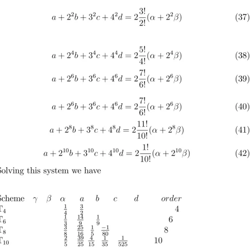
a + 22b + 32c + 42d = 23! 2!( + 2 2 ) (37) a + 24b + 34c + 44d = 25! 4!( + 2 4 ₎ ₍₃₈₎ a + 26b + 36c + 46d = 27! 6!( + 2 6 ₎ ₍₃₉₎ a + 26b + 36c + 46d = 27! 6!( + 2 6 ₎ ₍₄₀₎ a + 28b + 38c + 48d = 211! 10!( + 2 8 ₎ ₍₄₁₎ a + 210b + 310c + 410d = 2 1! 10!( + 2 10 ) (42)

Solving this system we have

Scheme a b c d order

T4 1₄ 3₂ 4

T6 1₃ 14₉ 1₉ 6

T8 3₈ 25₁₆ 1₅ ₈₀1 8

T10 2₅ 39₂₅ ₁₅4 ₃₅1 ₅₂₅1 10

Table 1. Coe¢ cients of interior schemes for …rst derivative

Scheme a b c d order T4 1 10 6 5 4 T6 2 11 12 11 3 11 6 T8 9 38 147 152 51 95 23 700 8 T10 8 29 1126 1305 988 1305 74 1015 43 9135 10

(22)

1.5 Adomian decompostion method

Usually numerical methods are based on discretization techniques, and only approximate values of the solution are obtained and only for some values of time and space. With Adomian decomposition method, the solution is obtained by a series expanssion of the so called Adomian’s polynomials, not requiring discretization of the variables, and, there-fore, not being a¤ected by errors associated to discretization. Also this method does not require linearization or perturbation and, consequently, does not change the actual solution of the problem. As well, Adomian’s decomposition method is very competent on …nding an approximate or exact solution for linear and non linear problems, not required in many cases, large computer memory.To introduce the Adomian decomposition method, consider the initial boundary value problem

ut r(a(x)ru) = G(x; t; u); x 2 2 R; t 2]0; T ] (43)

With the initial condition

u(x; 0) = u0(x); x2 (44)

Where G(x; t; u) is non linear vector function, some assumptions are taken for the data a; G; and u0 in order to assure the existence and

uniqueness of the solution of the system (1,45).

The principal algorithm of the Adomian decomposition method ap-plied to a general non linear equation is in the form

L(u) + R(u) + N (u) = q (45)

The linear term are decomposed into L+R, while the non linear terms are represented by N (u). L is taken as the highest order derivative, and R is the remainder of the linear operator. L 1 _{is regarded as the inverse}

operator of L and is de…ned by a de…nete integration from 0 to t, i.e., L 1(:) = Z t 0 (:)dt (46) If L a second-order operator L 1(:) = Z t 0 Z t 0 (:)dt dt (47)

(23)

Operating on both sides of equation (1,47) with the inverse operator L 1 yields

L 1(L(u)) = L 1(q) L 1(R(u)) L 1(N (u)) (49) Or

u(x; t) = u(x; 0) + tut(x; 0) + L 1(q) L 1(R(u)) L 1(N (u)) (50)

The decomposition method represents the solution of equation (1,32) as a series u(x; t) = 1 X n=0 un(x; t) (51)

The nonlinear operator, N (u), is decomposed as follows N (u)) =

1

X

n=0

An (52)

Substituting (1,33) and (1,34) into (1,32) we have

1 X n=0 un(x; t) = u0 L 1(R( 1 X n=0 un)) L 1( 1 X n=0 An) (53) Where u0 = u(x; 0) + tut(x; 0) + L 1(q) (54)

Consequently, it can be written as

u1 = L 1(R(u0)) L 1(A0) (55)

u2 = L 1(R(u1)) L 1(A1)

::

un+1 = L 1(R(un)) L 1(An)

Where An are Adomian’s polynomials of u0; u1; u2; :::; and are

ob-tained from the formula An = 1 n! dn d n[G( 1 X i=0 i ui)] =0; n = 0; 1; 2; ::: (56) Equation (1,38) gives A0 = g(u0) A1 = u1 d du0 g(u0)

(24)

A2 = u2 d du0 g(u0) + u2 1 2! d2 du2 0 g(u0) A3 = u3 d du0 g(u0) + u1u2 d2 du2 0 g(u0) + u3 1 3! d3 du3 0 g(u0) (57) :: :: ::

The accuracy level of the approximation of u(x; t) can be enhanced by computing components as far as we like. The n-term approximant

lim_n!1Sn= u(x; t); where (58)

Sn= n 1

X

k=0

uk(x; t); k 0

can be used to approximate the solution.

Conver

gence of the solution

We consider the following hypotheses

(H1) (T (u) T (v); v u) kku vk2; k > 0; u; v 2 H (59)

(H2) Whatever may be M > 0, there exists a constant C(M ) > 0

such that for u; v 2 H with kuk M, we have

(T (u) T (v); w) CM_ku v_{k kwk for every w 2 H} Where H is a Hilbert space.

Theorem. If N is lipschitzian function in H, the Adomian method applied to the following nonlinear heat equation

@u @t =

@2u

@x2 + g(u)

Where g(u) is the nonlinear terms converges.

Proof. We consider the above equation, then we set L(u) = @u @t; R(u) = @2_u @x2; N (u) = g(u) We have L(u) = @u @t = T (u) = @2_u @x2 + g(u)

(25)

This operator is hemicontinuous. We can the convergence hypothesis (H1) :ie.

There exists a constant k > 0, such that for u; v 2 H we have (T (u) T (v); u v) k_ku v_k2; T (u) T (v) = @ 2 @x2(u v) (g(u) g(v)); (T (u) T (v); u v) = ( @ 2 @x2(u v); u v) (g(u) g(v));

But there exists a real > 0 such that ( @ 2 @x2(u v); u v) ku vk 2 Because @2 @x2

Is a di¤erential operator in H. In addition , (g(u) g(v); u v) _ku v_k2 Where > 0 is the lipschitzian constant and therefore

(T (u) T (v); u v) ( )_ku v_k2;

And taking k = ; then we obtain hypothesis (H1), we can now

prove the hypothesis (H2), i.e.

8M > 0; • C(M) > 0 such that kuk kMk ; kvk M =₎ (T (u) T (v); w) C(M )_ku v_{k kwk ; 8w 2 H}

Thus we obtain

(T (u) T (v); w) _ku v_{k kwk + ku} v_{k kwk} C(M )_ku v_{k kwk}

(26)

1.6 The homtopy perturbation method

The explicit solutions of di¤erential equations are obtained by making use of reliable algorithm like homotopy perturbation method (HPM). In recent years, much attention has been given to the study of HPM ,He [13-17], and [23, 27, 29] for solving a wide range of problems whose mathematical models are governed by di¤erential equations or system of di¤erential equations. HPM deform a di¢ cult problem into an in…nite set of problems which are easier to solve without any need to transform nonlinear terms.The speed of convergence of the method is based on a rapidly convergent series with easily computable components. Numerical results show that the homotopy perturbation method is easy to imple-ment and accurate when applied to solve Partial di¤erential equations. to illustrate the basic ideas of this method, we consider the following equation:

L[u(x; t)] + N [u(x; t)] = q(x; t); (x; t)₂ (60) Subject to the boundary condition

B(u;@u

@ ) = 0; (x; t)2 And initial condition

u(x; 0) = u0 (61)

Where L is a linear operator, N a nonlinear operator and q(x; t) is the source term, B is a boundary operator and is the boundary of the domain . we de…ne a convex homotopy H(u; p) by

H(u; p) = (1 p)[L(v) L(u0)] + p[L(u) + N (u) q(x; t)] = 0 (62)

We have

H(u; 0) = L(v) L(u0) (63)

H(u; 1) = L(u) + N (u) q(x; t) (64) This shows that H(u; p) continuously traces an implicitly de…ned curve from a starting point H(v0; 0) to a solution function H(f; 1). The

embedding parameter monotonically increases from zero to unit as the trivial problem

L(v) L(u0) = 0

Continuously deforms the original problem L(u) + N (u) q(x; t) = 0

(27)

The embedding parameter p 2 [0; 1] can be considered as an expand-ing parameter [13-14,17]. We can assume that the solution of equation (44) can be written as a power series in p, as following

v = v0+ v1+ v2+ v3+ ::: (65)

The comparison of like powers of p give solutions of various orders and the best approximation is u = lim_p!1v = v0+ v1+ v2 + v3+ :::

It constitutes a main objective of this thesis to perform a numeri-cal analysis of heat equation with nonlonumeri-cal boundary conditions in both cases one-dimensional, two-dimensional and three-dimensional and wave equation , studying its solutions and behaviour by di¤erent numerical methods, namely High- order …nite di¢ rence method, Adomian’s de-composition method and homotopy perturbation method. In the second chapter we used the sixth-order …nite di¤erence scheme for solving a one dimensional di¤usion equation with an integral boundary condition, the obtained results are of order O(h6

x +h4t) [6]. in the last six chapters we

used the Adomian’s decompsition method and homotopy perturbation method, the obtained results are all exact [1-5].

(28)

(29)

2 A one-dimensional di¤usion equation with an

in-tegral condition

In this chapter, we …rst introduce the compact sixth-order …nite di¤er-ence formula then we adjust compact …nite di¤erdi¤er-ence formula for the following heat equation with non local boundary conditions

@u @t = @2_u @x2; (x; t)2]0; 1[ ]0; T [ (66) u(x; 0) = f (x); 0 < x < 1 (67) ux(1; t) = g(t); 0 < t < T (68) Z b 0 u(x; t)dx = m(t) (69)

where f (x), g(t), b and m(t) are known. This problem describe cer-tain chemicals absorbing light at various frequencies. The intensity of such light on photoelectric cell gives us an electric signal which is pro-portional to the total amount of chemical present in the volume through which the light passes. Let u(x; t) denote the chemical concentration which is di¤using in a straight glasse tube with x measured in the di-rection of axis of the tube. Then the electric signal produced by a light beam passing through the tube at right angles between x = 0 and x = b is proportional to R₀bu(x; t)dx. This integral represents the total mass of chemical in 0 x b at time t [18]. For such di¤usion processes, the integral condition (4) aries naturally and can be used as supplementary information in the determination of unknown concentration u(x; t).

J.cannon and J.vander hoek [49] studied the existence and uniqueness propreties of this problem.

A.B gumel [30] has proposed numerical scheme of order O(h2 x+ h2t)

L0_Stable parallel Algorithm for solving this problem.

Later, M.Akram and pasha [18] have proposed a more accurate al-gorithm of order O(h3

x + h3t). We propose a more accurate scheme of

order O(h6

x+ h4t). The numerical experiments show that the proposed

sixth-order schemes are unconditionally stable and more accurate than that in [18], furthermore for the choice

hx = 1₈ and ht= ₁₀₀₀1

The approximate solution coincides with the exact one at more than half of grid points discretization.

(30)

2.1 SIXTH-ORDER COMPACT FINITE

DIFFER-ENCE FORMULA

Compact formula is a special …nite di¤erence method which uses the values of the function and its derivatives only a

three consecutive points.

First keeping time continuous, we carry out a spatial discretization of @_@x2U2; we divide the interval [0; 1] using a uniform grid 0 = x0 < x1 <

x2 < :::::: < xN

with a mesh size hx= xi+1 xi = _N1; i = 0; 1; 2; :::::; N 1; N:

2.2 STANDARD COMPACT FINITE DIFFERENCE

The standard sixth-order compact …nite di¤erence formula for second derivative is h2 x 12(U 00 x2_{i 1}+ 10U_x002_i+ U_x002 i+1) = Ui 1 2Ui+ Ui+1) (70) where Ui = U (xi; t) and the coe¢ cients can be determined in the

following way.

1- Write the compact …nite di¤erence formula in general form

h2_x(a 1Ui 1" + a0Ui"+ a1Ui+1" ) = b 1Ui 1+ b0Ui+ b1Ui+1 (71)

where a 1; a0; a1; b 1; b0 and b1 are parameters to be determined.

2- Expand botIh sides of the equation (2.6) using Taylor series at the point xi

with respect to the discretization parameter hx:

3- We obtain six equations by setting the coe¢ cients hj

x; j =

0; 1; :::; 5

equal zero.solve the six equations for the six unknown parameters. The obtained accuracy is O(h6

x) for formula (2.6)

2.2- Write equation (2.1) in a discret point form @u(xi; t) @t = @2_u(x i; t) @x2 i ; i = 1; ::::; N 1 (72) Equation (2.5) is valid only for i = 2; 3,...,N 2to attain the same accuracy at i = 1

(31)

and i = N 1 special formula must be developed. When i = 1 we use the formula

h2 x 12(14U " 1 5U " 2 + 4U " 3 U " 4) = U0 2U1+ U2 (73)

From Simpson integration Rule we have_R

b

0 u(x; t)dx t hx

3 (u0+ 4u1+ u2) = m(t);

b has been chosen as a grid point, and when i=N-1 we use the formula h2 x 12( 127 30 U " N 4+ 86 5 U " N 3 257 10 U " N 2+ 461 15 U " N 1) = UN 2 UN 1+hU 0 N (74) We use U to stand for the approximation value of u throughout this chapter.

All Formula are O(h6

x) or written in Matrix Form

AU " = M U + H (75) Where A = h2x 12 2 6 6 6 6 6 6 6 6 6 6 6 6 6 6 4 14 5 4 1 0 0 : : : 0 1 10 1 0 0 : : : : 0 0 1 10 1 0 0 : : : 0 0 0 1 10 1 0 0 : : 0 0 0 0 1 10 1 0 0 : 0 0 : : 0 1 10 1 0 : 0 0 : : : 0 1 10 1 0 0 0 : : : : 0 1 10 1 0 0 : : : : : 0 1 10 0 0 : : : : 0 127 30 86 5 257 10 461 15 3 7 7 7 7 7 7 7 7 7 7 7 7 7 7 5 M = 2 6 6 6 6 6 6 6 6 6 6 6 6 6 6 4 6 0 0 : : : : : : 0 1 2 1 0 0 : : : : 0 0 1 2 1 0 0 : : : 0 0 0 1 2 1 0 0 : : 0 0 0 0 1 2 1 0 : : 0 0 : : 0 1 2 1 0 : 0 0 : : : 0 1 2 1 0 0 0 : : : : 0 1 2 1 0 0 : : : : : 0 1 2 1 0 : : : : : : 0 1 1 3 7 7 7 7 7 7 7 7 7 7 7 7 7 7 5 ; H = 2 6 6 6 6 6 6 6 6 6 6 6 6 6 6 4 3 hm(t) 0 : : : : : : 0 hU0 N 3 7 7 7 7 7 7 7 7 7 7 7 7 7 7 5 :

(32)

Finally, we obtain

U " = A 1M U + A 1H Putting A 1_{M = B} _{and A} 1_{H = R(t)}

U " = B U (t) + R(t ) (76) Substituting in (2.7) we get a system of ordinary di¤erential equations

dU

dt = B U (t) + R(t) (77)

with the initial condition

U (0) = f (x)

Putting f (t; U ) = B U (t) + R(t), we obtain the following equation

dU

dt = f (t; U ) (78)

We solve this equation using fourth-order Runge-Kutta Method as followning k1 = f (t0; U0) k2 = f (t0+1₂ht;K₂1htU0) k3 = f (t0+1₂ht;K₂2htU0) k4 = f (t0+ ht; k3ht+ U0) UN +1 = UN + 1 6ht(k1+ 2k2+ 2k3+ k4) (79)

2.3 COMPUTATIONAL RESULTS

In order to test the sixth-order compact …nite di¤erence scheme, we consider the problem. Consider the heat

equation with f (x) = 0:5x2 g(t) = 1

m(t) = 0:75t + 1₆(0:75)3

which is easily seen to have exact solution u(x; t) = 0:5x2+ t: Using Runge-Kutta method, the problem is solved for

hx=1₈; ht= ₁₀₀₀1 ; hx = ₁₀1 ; ht= ₁₀₀₀1

The results of approximate solution are tabulated in Tables 1 and 2

(33)

hx = 1₈; ht= ₁₀₀₀1

x exact solution approximate solution absolute error

1 8 8:8125 10 3 _8:3865 ₁₀ 2 _7:5053 ₁₀ 2 1 4 0:03225 2:8182 10 2 _4:068 ₁₀ 3 3 8 7:1313 10 2 _7:1477 ₁₀ 2 _1:64 ₁₀ 4 1 2 0:126 0:126 0:0 5 8 0:19631 0:19631 0:0 3 4 0:28225 0:28225 0:0 7 8 0:38381 0:38381 0:0 T able 1 hx = ₁₀1; ht = ₁₀₀₀1

x exact solution approximate solution absolute error

1 10 0:006 0:14449 0:13849 1 5 0:021 1:7083 10 2 _3:917 ₁₀ 3 3 10 0:046 4:5849 10 2 _1:51 ₁₀ 4 2 5 0:081 8:10446 10 2 _4:46 ₁₀ 5 1 2 0:126 0:126 0:0 3 5 0:181 0:181 0:0 7 10 0:246 0:246 0:0 4 5 0:321 0:321 0:0 9 10 0:406 0:406 0:0 T able 2

Conclusion

It is observed that the results obtained using compact sixth-order …nite di¤erence scheme are unconditionally stable and highly accurate and more e¢ cient if compared to those obtained by Akram and Pasha [18]. the method developed is sixth-order accurate in space and fourth-order in time with very high speed fourth-fourth-order Runge-Kutta Algorithm. It should to be noted that, only one iterate was needed to obtain the results shown in both tables 1 and 2.

(34)

uex= 0:5x + t 1 0 1.0 0 0.8 0.6 0.4 x 0.0 0.2 z ₂3 4 1 y 4 3 2 5

(35)

2.4 One-dimensional nonhomogeneous heat

equa-tion with nonlocal boundary condiequa-tions

Statement of the Problem

In this chapter, we consider the non homogeneous heat equation in one dimension with the non local boundary conditions. There has re-cently been much attention to the search for better and more accurate solution methods for determining a solution, approximate or exact to this type of problems. Consider the heat equation

@u @t =

@2_u

@x2 + q(x; t); 0 < x < 1; 0 < t T (80)

Subject to the given initial condition

u(x; 0) = f (x); 0 x 1 (81)

And the non local boundary conditions u(0; t) = Z 1 0 (x; t)u(x; t)dx + g(t)1; 0 < t T (82) u(1; t) = Z 1 0 (x; t)u(x; t)dx + g(t)2; 0 < t T (83)

where f ,g1; g2; ; and qare known functions and are su¤eciently smooth,

T is given constant. Many authors as [6] , [9] [18-22] ,[30-31] and [24-26], have suggested traditional techniques for solving this type of problems in M. A. Rahman [8], has proposed a fourth-order numerical …nite dif-ference scheme for the solution of this problem. We propose a new tech-nique for solving the given problem, this techtech-nique is based on Adomian’s series solution method. This method provides us an exact solution which is much better result than that in [8]

.

2.5 Adomian Decomposition Method

To introduce the Adomian decomposition method, consider the problem @u @t = @ @x(k(x) @u @x) + G(x; t; u); x2 R; t2 (0; T ] (84) With the initial condition

(36)

And the nonlocal boundary conditions u(0; t) = Z 1 0 '(x; t)u(x; t)dx + g(t)1; 0 < t T (86) u(1; t) = Z 1 0 (x; t)u(x; t)dx + g(t)2; 0 < t T (87)

Where G(x; t; u) is nonlinear function, assuming that su¢ ciently smooth in order to assure the existence and uniqueness of the solution to the equation (2,1)

In this section, we outline the steps to obtain a solution of (3,1)-(3,4) using Adomian decomposition method, which is initiated by G.Adomian[36], [40],and [47]. To begin it is convenient to rewrite the problem in the standard form

Lt(u) = Lxx(u) + q(x; t) (88)

Where the di¤erential operators Lt and Lxx are given by

Lt(:) = _@t@(:) and Lxx = @

2

@x2:

Assuming that the inverse operator Lt1 exists and it is de…ned as

L_t1 = Z t

0

(:)dt (89)

Applying inverse operator Lt1 on both sides of (3; 5) and using the

initial condition yields

L_t1(Lt(u)) = Lt1(Lxx(u)) + Lt1(q(x; t))

Or

u(x; t) = f (x) + L_t1(Lxx(u)) + Lt1(q(x; t))

Now we decompose the unkown function u(x; t) by a sum of components de…ned by the series [36]

u(x; t) =

1

X

k=0

uk(x; t) (90)

Where u0 is identi…ed as u(x; 0) , the components uk(x; t) are obtained

by the recursive formula

1 X k=0 uk(x; t) = f (x) + Lt1fLxx( 1 X k=0 uk(x; t))g + Lt1(q(x; t)) Or u0(x; t) = f (x) + Lt1(q(x; t)) (91)

(37)

uk+1(x; t) = Lt1(Lxx(uk(x; t))); k 0 (92)

We note that the recursive relationship is constructed on the basis that the zeroth component u0(x; t) is de…ned by all terms that arise from

the initial condition and from integrating the source term,the remaining components uk(x; t); k 1;can be completly determined such that each

term is computed by using the previous term. Accordingly, considering few terms only the relations (3,8) and (3,9) give

u0 = f (x) + Lt1(x; t)

u1 = Lt1(Lxx(u0))

u2 = Lt1(Lxx(u1))

and so on. As a result, the components u0 ,u1;u2,... are identi…ed and

the series solution thus entirely determined. However, in many cases the exact solution in a closed form may be obtained as we can see in our examples.

2.6 Numerical Examples

EXAM P LE 1 we consider the problem (3; 1) with;

f (x) = x2; 0 < x < 1; g1(t) = 1 4(t + 1)2; 0 < t < 1 (93) g2(t) = 3 4(t + 1)2; 0 < t < 1; (x; t) = x; 0 < x < 1 (94) (x; t) = x; 0 < x < 1; q(x; t) = 2(x_(t+1)2+t+1)3 ; 0 < x < 1; 0 < t 1

which has exact solution u(x; t) = ( x t+1)

2_{, we rewrite the given}

prob-lem in an operator form

Lt(u(x; t)) = Lxx(u(x; t)) + q(x; t) (95) where Lt(:) = _@t@(:),Lxx = @ 2 @x2(:),L 1 t = Rt 0(:)dt

Applying the inverse operator Lt1on both sides of (3,12) we have

u(x; t) = u(x; 0) + L_t1(Lxx(u(x; t))) + Lt1(q(x; t)) (96)

Now the recursive formula is

(38)

Or u0 = x2+ Lt1f 2(x2+ t + 1) (t + 1)3 g And uk+1(x; t) = Lt1(Lxx(uk(x; t))); k 0 (97)

Using the recursive relation we compute the components as follows u0 = x2+ Z t 0 2(x2+ t + 1)dt (t + 1)3 = x2 (t + 1)2 + 2 t + 1 2 (98) u1 = Lt1(Lxx(u0)) = Z t 0 2dt (t + 1)2 = 2 t + 1 + 2 uk = 0; k 2 (99)

The solution in the series form is given by u(x; t) = 1 X k=0 u(x; t) Or u(x; t) = u0(x; t) + u1(x; t) + uk(x; t); k 2

Hence, the solution of (3,1) with (3,10) and (3,11) is given as u(x; t) = x

2

(t + 1)2

which is the exact solution.

EXAM P LE 2 In this example we consider

q(x; t) = 0 (100) u(x; 0) = f (x) = 0:5x2; 0 < x < 1 (101) ux(1; t) = g(t) = 1; 0 < t < T Z b 0 u(x; t)dx = m(t) = 0:75t +1 6(0:75) 3 ₍₁₀₂₎

where b is belongs to ]0; 1[. We rewrite the given problem in an operator form as

Lt(u(x; t)) = Lxx(u(x; t)) + q(x; t) (103)

(39)

Lt(:) = _@t@(:); Lxx = @ 2 @x2; L 1 t = Rt 0(:)dt:

Applying the inverse operator Lt1 on both sides of (3,20), we have

u(x; t) = u(x; 0) + L_t1(Lxx(u(x; t))) + Lt1(q(x; t) (104)

u0(x; t) = f (x) + Lt1(0)

Or

u0(x; t) = 0:5x2+ Lt1(0)

And

uk+1(x; t) = Lt1(Lxx(uk(x; t))); k 0

Using the recursive relation we compute the components as follows

u0(x; t) = 0:5x2 (105) u1(x; t) = Lt1(Lxx(u0(x; t)) Or u1(x; t) = Z t 0 dt = t (106) uk(x; t) = 0; k 2 (107)

Thus, the solution in series form is given by u(x; t) = 1 X k=0 uk(x; t) Or u(x; t) = u0(x; t) + u1(x; t) + uk(x; t); k 2

Hence, the solution of (3,1) with (16-19) is given as u(x; t) = 0:5x2+ t

This solution coincides with the exact one.

EXAM P LE 3 consider the problem

q(x; t) = 30x4+ 6t5

(40)

u(0; t) = Z 1 0 (x; t)u(x; t)dx+g1(t); 0 t T u(1; t) = Z 1 0 (x; t)u(x; t)dx + g2(t); 0 t T Where (x; t) = 0:2; (x; t) = 0:4 g1(t) = 4 5t 6 1 35; g2(t) = 3 5t 6₊ 33 35

Applying the inverse operator Lt1 on both sides of (3,1), we have

u0(x; t) = f (x) + Lt1(q(x; t)) Or u0(x; t) = x6+ Lt1( 30x 4_{+ 6t}5₎ And uk+1(x; t) = Lt1(Lxx(uk(x; t))); k 0

Computing the components u0; u1; u2 and u3

u0(x; t) = x6+Lt1( 30x 4_+6t5_{) = x}6₊ Z t 0 ( 30x4+6t5)dt = x6 30x4t+t6 u1 = Lt1(Lxx(u0)) = Lt1(30x 4 _360x2_{t) =} Z t 0 (30x4 360x2t)dt = 30x4t 180x2t2 u2 = Lt1(Lxx(u1)) = Lt1(360x 2_{t 360t}2_{) =} Z t 0 (360x2t 360t2)dt = 180x2t2 120t3 u3 = Lt1(Lxx(u2)) = Lt1(360t 2 ) = Z t 0 360t2dt = 120t3 uk = 0; k 4

Finally, we obtain the solution

u(x; t) = u0+ u1+ u2+ u3

Or

(41)

This solution coincides with the exact one. Example 4

Consider solving the di¤usion equation @u @t = @2_u @x2 + ( 2_{+ 1)e}t_{sin( x); x} 2 (0; 1); t 2 (0; 1) u(0; t) = u(1; t) = 0 (109) u(x; 0) = sin( x) The exact solution of this equation is

u(x; t) = etsin( x)

to solve this problem we write it in an operator form as

Ltu(x; t) = Lxx(u(x; t)) + ( 2+ 1)etsin( x) (110)

Operating L_t1 on both sides of (3,27) and imposing the initial con-dition we obtain

u(x; t) = u(x; 0) + L_t1(Lxx(u(x; t))) + Lt1(( 2+ 1)etsin( x)) (111)

Where L_t1 is a one fold integral operator, which means that L_t1 =

Z t 0

(:)dt

The Adomian decomposition method assumes a series solution for u(x; t) given by an in…nite sum of components

u(x; t) =

1

X

k=0

uk(x; t) (112)

The components uk(x; t) are computed recursively as follows

u0(x; t) = sin( x) + Lt1((

2_{+ 1)e}t_{sin( x))} ₍₁₁₃₎

And

uk+1(x; t) = Lt1(Lxx(uk(x; t)); k 0 (114)

To …nd the solution , one solves the above recursive relations respec-tively, we obtain

u0(x; t) = sin( x) +

Z t 0

(42)

u0(x; t) = 2sin( x) + ( 2+ 1)etsin( x)

u1(x; t) = Lt1(Lxx(u0(x; t)) =

Z t 0

( 4sin( x) ( 2+ 1) 2etsin( x))dt u1(x; t) = ( 2+ 1) 2sin( x) + 4sin( x)t 2( 2 + 1)sin( x)et

u2(x; t) = Lt1(Lxx(u1(x; t)) =

Z t 0

( 6sin( x))t 4( 2+1)sin( x)+ 4( 2+1)sin( x)et)dt

u2(x; t) = 4( 2+1)sin( x) 4( 2+1)(sin( x))t ( 6sin( x))

t2 2!+( 4₍ 2_{+1)sin( x))e}t u3(x; t) = Lt1(Lxx(u2(x; t)) = Z t 0

( 6( 2+1)sin( x)+ 6( 2+1)sin( x)t+ 8sin( x)t

2

2!

6₍ 2_+1)et_{sin x)dt}

u3(x; t) = 6( 2+1)sin( x)+ 6( 2+1)sin( x)t+ 6( 2+1)sin( x)

t2 2!+ 8_{sin( x)}t3 3! 6₍ 2_{+1)sin( x)e}t u4(x; t) = Lt1(Lxx(u3(x; t)) = Z t 0 Lxx(u3(x; t))dt

u4(x; t) = 8( 2+ 1)sin( x) 8( 2+ 1)(sin x)t 8( 2+ 1)sin x

t2 2! 8₍ 2_{+ 1)sin x}t 3 3! 10₍ 2_{+ 1)sin x}t4 4!+ 8₍ 2_{+ 1)(sin( x))e}t

u5(x; t) = 10( 2+ 1)sin( x) + 10( 2+ 1)sin( x)t + 10( 2+ 1)sin( x)

t2 2!+ 10₍ 2_{+ 1)sin x}t3 3!+ 10₍ 2_{+ 1)sin x}t4 4!+ 12₍ 2_{+ 1)sin x}t5 5! 10₍ 2_{+ 1)sin( x)e}t

u6(x; t) = 12( 2+ 1)sin( x) 12( 2+ 1)sin( x)t 12( 2+ 1)sin( x)

t2 2! 12₍ 2_{+ 1)sin x}t3 3! 12₍ 2_{+ 1)sin( x)}t 4 4! 12₍ 2_{+ 1)sin( x)}t 5 5! 12₍ 2_{+ 1)sin( x)}t 6 6! + + 12( 2+ 1)sin( x)et

And so on, then

u(x; t) = u0(x; t) + u1(x; t) + u2(x; t) + u3(x; t) + u4(x; t) + :::: = etsin( x)

(115) This result is in good agreement with analytic solution

.

(43)

We consider the problem (3,1)-(3,4) with:

u(x; 0) = f (x) = 2cos(x); 0 < x < 1 (116) And the boundary conditions

u(1; t) = g(t) = ( 2+ t)cos(1:0); 0 < t < 1 Z b

0

u(x; t)dt = ( 2+ t)sin(0:75); 0 < t < 1 (117) q(x; t) = (1 + 2 + t)cos(x)

b = 0:75, from equations (3,8) and (3,9) we obtain u0= 2cos(x) + Z t 0 (1 + 2+ t)cos(x)dt = 2cos(x) + (118) +(1 + 2)tcos(x) + t 2 2!cos(x) u1 = Lt1[Lxx(u0)] = 2tcos(x) (1 + 2) t2 2!cos(x) t3 3!cos(x) (119) u2 = Lt1[Lxx(u1)] = 2 t2 2!cos(x) + (1 + 2 )t 3 3!cos(x) + t4 4!cos(x) (120) u3 = Lt1[Lxx(u2)] = 2 t3 3!cos(x) (1 + 2₎t4 4!cos(x) t5 5!cos(x) (121) u4 = Lt1[Lxx(u3)] = 2 t4 4!cos(x) + (1 + 2₎t5 5!cos(x) + t6 6!cos(x) (122) u5 = Lt1[Lxx(u4)] = 2 t5 5!cos(x) (1 + 2₎t6 6!cos(x) t7 7!cos(x) (123) :::: And so on, un 2 = Lt1[Lxx(un 3)] = ( 1)n 2cos(x)[ 2 tn 2 (n 2)!+(1+ 2₎ tn 1 (n 1)!+ tn n!] (124) un 1 = Lt1[Lxx(un 2)] = ( 1)n 1cos(x)[ 2 tn 1 (n 1)!+(1+ 2₎tn n!+ tn+1 (n + 1)!] (125) un= Lt1[Lxx(un 1)] = ( 1)ncos(x)[ 2 tn n! + (1 + 2₎ tn+1 (n + 1)! + tn+2 (n + 2)! (126)

(44)

We sum the …rst n-terms, we have Sn= n X i=0 ui = ( 2+ t)cosx + ( 1)n[ 2 tn+1 (n + 1)! + tn+2 (n + 2)!]; 0 < t < 1 (127) Hence

u(x; t) = lim_n!1Sn = ( 2+ t)cos(x) (128)

This solution is in good agreement with the exact one.

2.7 Conclusion

In this chapter Adomian decomposition method is proposed for solving non homogeneous heat equation with nonlocal boundary conditions and initial condition. The results obtained show that the Adomian decom-position method provides us an exact solution.

(45)

Example 3 T able 1 hx = 1 10; ht = 1 100

Comparing absolute Error f or Adomian 4 terms

xi uAd uex juex uAdj 0 1:2000 10 4 1:0 10 12 1:2000 10 4 0:1 1:1900 10 4 1:0 10 6 1:18 10 4 0:2 5:6 10 5 6:4 10 5 0:00012 0:3 6:09 10 4 7:29 10 4 0:00012 0:4 3:976 10 3 4:096 10 3 0:00012 0:5 1:5505 10 2 1:5625 10 2 0:00012 0:6 4:6536 10 2 4:6656 10 2 0:00012 0:7 0:11753 0:11765 0:00012 0:8 0:26202 0:26214 0:00012 0:9 0:53132 0:53144 0:00012 1:0 0:99988 1:0 0:00012

(46)

Example 4 hx= 1 10; ht = 1 100 xi uex uAd 4 Iterates juex uAdj 0:0 0:0 0:0 0:0 0:1 0:34152 0:32905 0:01247 0:2 0:6496 0:62589 0:02371 0:3 0:8941 0:86147 0:03263 0:4 1:0511 1:0127 0:0384 0:5 1:1052 1:0648 0:0404 0:6 1:0511 1:0127 0:0384 0:7 0:8941 0:86147 0:03263 0:8 0:6496 0:62589 0:02371 0:9 0:34152 0:32905 0:01247 1:0 0:0 0:0 0:0

(47)

Example 5 hx= 1 10; ht= 1 25 xi uex 4 iterates uAd juex uAdj 0:0 9:9096 9:9096 0:0 0:1 9:8601 9:8601 0:0 0:2 9:7121 9:7121 0:0 0:3 9:467 9:467 0:0 0:4 9:1274 9:1274 0:0 0:5 8:6965 8:6965 0:0 0:6 8:1787 8:1787 0:0 0:7 7:5793 7:5793 0:0 0:8 6:9041 6:9041 0:0 0:9 6:1599 6:1599 0:0 1:0 5:3542 5:3542 0:0

(48)

uex= x 2 (t+1)2 1.0 1.0 0.8 0.8 0.6 0.6 x y 0.2 0.2 0.4 0.4 0.0 0.0 0.0 0.2 0.4 z 0.6 0.8 1.0 Variation of uex= x 2

(49)

uex= x6+ t6 -4 y -2 4 2 _x 0 -4 -2 0 2 0 4 10000 z 20000 30000

(50)

uAd= x6+ t6 120t3 -4 -2 y 4 -4 x 2 0 0 0 -2 2 4 10000 20000 30000 z 40000

(51)

uex= exp(t) sin( x) -10 -20 -6 -4 -2 20 y10 0 0 2 0 z 4 5 2 3 6 4x 1

(52)

u = 8 _{sin( x)} _{( 4:2514} ₁₀ 6_{) + exp(t)} _{sin( x)} -10 -20 -6 -4 20 y -2 10 0 0 2 0 z 5 2 3 4 1 x 4 6

Variation of uAd = ( 4:2514 10 6) 8sin( x) + sin( x) exp(t) for

(53)

T able 2 Comparing Absolute Error hx=

1

10; ht= 1 100

F or 4 terms of Adomian solution

x uAd uex juex uAdj 0:0 0:0 0:0 0:0 0:1 0:4 0:31214 0:08786 0:2 0:6 0:59373 0:00627 0:3 0:8 0:81719 0:101719 0:4 0:9 0:96067 0:06067 0:5 1:0 1:0101 0:0101 0:6 0:9 0:96067 0:06067 0:7 0:8 0:81719 0:01719 0:8 0:6 0:59373 0:00627 0:9 0:4 0:31214 0:08786 1:0 0:0 0:0 0:0

(54)

Example 5 hx= 1 10; ht = 0:25 xi uex 4 Iterates uAd juex uAdj 0:0 9:9096 9:9096 0:0 0:1 9:8601 9:8601 0:0 0:2 9:7121 9:7121 0:0 0:3 9:467 9:467 0:0 0:4 9:1274 9:1274 0:0 0:5 8:6965 8:6965 0:0 0:6 8:1787 8:1787 0:0 0:7 7:5793 7:5793 0:0 0:8 6:9041 6:9041 0:0 0:9 6:1599 6:1699 0:0 1:0 5:3542 5:3542 0:0

(55)

uex= ( 2 + t) cos(x) -10 0 x -4 -5 -2 y z 2 4 0 0 4 2 5 -2 10 _-4

(56)

uAd= ( 2 + t) cos(x) t 5 120 -4 -40 -20 -2 z y 4 2 0 0 0 x 2 -2 4 -4 20 Variation of uAd= ( 2+ t) cos(x) t 5

(57)

2.8 One-dimensional nonhomogeneous di¤usion

equa-tion with derivative boundary condiequa-tions

Statement of the Problem

In this chapter, we consider the one dimensional nonhomogeneous heat equation with derivative boundary conditions

@u @t = @2u @x2 + q(x; t); (x; t) ]0; 1[ ]0; T [ (129) u(x; 0) = g(x); 0 x 1 (130) ux(0; t) = f1(t); 0 < t T (131) ux(1; t) = f2(t); 0 < t T (132)

Where g(x); f1(t); f2(t) and q(x; t) are known. Many authors have

proposed numerical methods for solving nonlocal problems [6], [7-10], [18-22], [24-26], [30-31]. Later Akram[11], has proposed an 0(h3 _{+ t}3₎

L0 stable parallel algorithm for solving the problem. In this work we

propose a new technique based on the Adomian decomposition series solution [36,40,47]. The numerical examples show that results obtained coincide with the exact ones [1]. The organization of this chapter is the following.

In this section, we give a brief de…nition of this method, in section 3 the accuracy and the e¤eciency of the Adomian decomposition method are investigated with numerical illustration, the section 4 consists of a brief conclusion.

2.9 Adomian decomposition method

Reweriting the problem (4,1) in the following operator form

Lt(u(x; t)) = Lxx(u(x; t)) + q(x; t) (133) where Lt(:) = @ @t(:); Lxx(:) = @2 @x2(:)

L 1_{is regarded as the inverse operator of L and is de…ned by a de…ned}

integration from 0 to t, i.e.

L_t1(:) = Z t

0

(58)

Operating on both sides of equation (4,5) with Lt1 using the initial

condition yields

L_t1Lt(u(x; t)) = Lt1(Lxx(u(x; t))) + Lt1(q(x; t))

Or

Now we decompose the unkown function u(x; t) by a sum of compo-nents de…ned by the following series with u0 identi…ed as u(x; 0)

u(x; t) =

1

X

k=0

uk(x; t) (136)

The components uk are obtained by the recursive formula 1 X k=0 uk(x; t) = g(x) + Lt1(Lxx( 1 X k=0 uk(x; t))) + Lt1(q(x; t)) Or u0 = g(x) + Lt1(q(x; t)) (137) uk+1 = Lt1(Lxx(uk(x; t))); k 0 (138)

From the equations (4,9) and (4,10), we get u0 = g(x) + Lt1(q(x; t))

u1 = Lt1(Lxx(u0(x; t)))

u2 = Lt1(Lxx(u1(x; t)))

u3 = Lt1(Lxx(u2(x; t)))

:::::::::::::::::::::::::

and so on. The componenets u0,u1; u2; u3; :::::; are identi…ed and the

series solution thus entirely determined. However in many cases the exact solution in a closed form may be obtained. For numerical purposes, we can use the approximation

u(x; t) = lim_{m !1} _m (139) where m = m 1_X k=0 uk(x; t) (140)

Evaluating more componenets of u(x; t); we obtain a more accurate solution. Noting that the convergence of this method has been proved by Adomian [47], Adomian and Rach[40] and Wazwaz [32] have investi-gated the phenomenon of the self-canceling "Noise" terms where sum of components vanishes in the limit, we observe that "Noise" terms appear for nonhomogeneouse cases only.

(59)

2.10 Numerical examples

Example 1

We consider the nonhomogeneous heat equation @u @t = @2_u @x2 + q(x; t); 0 < x < 1; t > 0 (141) q(x; t) = 2ex t ux(0; t) = f1(t) = e t; 0 < t T ux(1; t) = f2(t) = e1 t; 0 < t T u(x; 0) = g(x) = ex; 0 x 1 (142) Rewriting equation (4,13) in operator form

Lt(u(x; t)) = Lxx(u(x; t))) + q(x; t) (143) where Lt(:) = @ @t(:); Lxx(:) = @2 @2(:); L 1 t (:) = Z t 0 (:)dt Applying Lt1 on both sides of (4,15), we have

Now we get the recursive formula as follows u0(x; t) = g(x) + Lt1(q(x; t)) Or u0(x; t) = ex+ Lt1( 2e x t_{) = e}x_{( 1 + 2e} t₎ ₍₁₄₅₎ uk+1(x; t) = Lt1(Lxx(uk(x; t))); k 0 u1(x; t) = Lt1(Lxx(u0(x; t))) = ex(2 t 2e t) (146) u2(x; t) = Lt1(Lxx(u1(x; t))) = ex( 2 + 2t t2 2 + 2e t₎ ₍₁₄₇₎ u3(x; t) = Lt1(Lxx(u2(x; t))) = ex(2 2t + t2 t3 3! 2e t₎

Then the solution, in the series form, is given by u(x; t) =

1

X

k=0

(60)

Or u(x; t) = ex(1 t + t 2 2! t3 3! + :::) = e x t

This solution is the exact one. Example 2

Consider the problem (1) with the follownig conditions q(x; t) = xt2

u(x; 0) = sin(x) (148)

ux(0; t) = 1

ux(1; t) = sin(t)

Rewriting the given problem in an operator form as

Lt(u(x; t)) = Lxx(u(x; t)) + q(x; t) (149) where Lt(:) = @ @t(:); Lxx(:) = @2 @x2(:) and L 1 t (:) = Z t 0 (:)dt

Applying the inverse operator Lt1on both sides of equation (4,21),

we get

u0(x; t) = g(x) + Lt1(q(x; t)) Or u0(x; t) = sin(x) + Z t 0 xt2dt = sin(x) + x(t 3 3) (151) uk+1(x; t) = Lt1(Lxx(u(x; t))); k 0 Then u1(x; t) = Lt1(Lxx(u(x; t))) = Z t 0 sin(x)dt = t sin(x) (152) u2(x; t) = Lt1(Lxx(u1(x; t))) = Z t 0 tsin(x)dt = t 2 2!sin(x) (153)

(61)

u3(x; t) = Lt1(Lxx(u2(x; t))) = Z t 0 t2 2sin(x)dt = t3 3!sin(x) (154) :::::::::::::::::::

And so on, the solution in the series formula is given by u(x; t) = 1 X k=0 uk(x; t) Or u(x; t) = t 3 3x + (1 t 1!+ t2 2! t3 3!+ :::)sin(x) = t3 3x + e t_sin(x) ₍₁₅₅₎

this is the exact solution. Example 3

Consider the problem (1) with the following boundary and initial conditions q(x; t) = 0 u(x; 0) = sin( x) (156) ux(0; t) = e 2_t ux(1; t) = e 2_t

We rewrite the equation (1) in an operator form as following

Lt(u(x; t)) = Lxx(u(x; t)) + q(x; t) (157) where Lt(:) = @ @t(:); Lxx(:) = @2 @x2 and L 1 t (:) = Z t 0 (:)dt

Operating on both sides of equation (4,28) with the inverse operator L_t1; we have

Proceeding as before, we …nd the recursive formula as follows u0(x; t) = g(x) + Lt1(q(x; t))

Or

u0(x; t) = sin( x)

(62)

So, the components of the series solution are computed using the recursive formula as follows

u0(x; t) = sin( x) (159) u1(x; t) = Lt1(Lxx(u0(x; t))) = 2tsin( x) u2(x; t) = Lt1(Lxx(u1(x; t))) = t2 2! 4_{sin( x)} u3(x; t) = Lt1(Lxx(u2(x; t))) = t3 3! 6_{sin( x)} ::::::::

And so on, the solution in the series formula is given by

u(x; t) = 1 X k=0 uk(x; t) Or u(x; t) = sin( x)(1 2_t 1! + 4_t2 2! 6_t3 3! + :::) = sin( x)e 2_t

This solution coincides with the analytic one. .EXAMPLE 4

Consider the heat equation @u

@t

@2u

@x2 = 0; 0 < x < 1 (160)

Subjec to the intial condition

u(x; 0) = sinx; 0 < x < 1 (161) and the boundary conditions

ux(1; t) = e 2_t ; 0 < t < T Z b 0 u(x; t)dx = 1(_p₂1 2+ 1)e 2_t (162) we rewrite the equation (4,31) in an operator form

(63)

Following Adomian, appliyng the inverse operator Lt1 to both sides

of equation (4,34) one obtains

u(x; t) = u0(x; 0) + Lt1(Lxx(u(x; t)) (164)

According to Adomian’s method, one assumes that the unknown function u(x; t) can be expressed by an in…nite sum of components of the form, u(x; t) = 1 X n=0 un(x; t) (165)

Substituting equation (4,36) into equation (4,35) one obtains

1 X n=0 un(x; t) = u0(x; 0) + Lt1(Lxx( 1 X n=0 un(x; t))) (166)

To determine the components of un(x; t); n = 0; 1; 2; :::; Adomian’s

technique can employ the recursive relation de…ned by

u0 = u0(x) = sinx (167) u1 = Lt1(Lxx(u0)) = Z t 0 sinxdt = tsinx (168) u2 = Lt1(Lxx(u1)) = sinx Z t 0 tdt = t 2 2!sinx (169) u3 = Lt1(Lxx(u2)) = sinx Z t 0 t2 2!dt = t3 3!sinx (170) :::

And so on, the solution obtained is given by u(x; t) = u0+u1+u2+u3+:::+: = sinx(1 t+ t2 2! t3 3!+::+::) = e t_sinx (171)

2.11 Conclusion

The results obtained in this chapter compared to those obtained by Akram[11] show that the Adomian decomposition method is more accu-rate. In adddition the computation of the components of the solution are easy and take less time in comparison with other classical methods.

(64)

Example 1 hx= 1 10; ht = 1 25 xi uex 4 Iterates uAd juex uAdj 0:0 0:96079 0:96079 0:0 0:1 1:0618 1:0618 0:0 0:2 1:1735 1:1735 0:0 0:3 1:2969 1:2969 0:0 0:4 1:4333 1:4333 0:0 0:5 1:5841 1:5841 0:0 0:6 1:7507 1:7507 0:0 0:7 1:9348 1:9348 0:0 0:8 2:1383 2:1383 0:0 0:9 2:3632 2:3632 0:0 1:0 2:1617 2:1617 0:0

(65)

Example 2 hx= 1 10; ht= 1 25 xi uex uAd 4 Iterates juex uAdj 0:0 0:0 0:0 0:0 0:1 0:10391 9:5921 10 2 7:989 10 3 0:2 0:20678 0:19088 0:0159 0:3 0:30759 0:28394 0:02365 0:4 0:40532 0:37416 0:03116 0:5 0:499 0:46064 0:03836 0:6 0:58770 0:54252 0:04518 0:7 0:67052 0:61897 0:05155 0:8 0:74665 0:68925 0:0574 0:9 0:81531 0:75263 0:06268 1:0 0:87583 0:80850 0:06733

(66)

uex= exp(x t) 1.0 0.8 0.6 0.4 z 1.4 0.2 1.0 0 1.2 1.6 0.0 2 1 x y 3 2.0 1.8 4 5

(67)

uAd= exp(x) (1 t + t 2 2! t3 3!) 1.0 0.8 0.6 0.4 z 0 1.2 1.4 1.0 0.2 1.6 0.0 2 1 x y 3 2.0 1.8 4 5 Variation of uAd = exp(x) (1 ₁t + t 2 2! t3

3!) for di¤erent values of