HAL Id: hal-01579422
https://hal.inria.fr/hal-01579422
Submitted on 31 Aug 2017
HAL is a multi-disciplinary open access
archive for the deposit and dissemination of sci-entific research documents, whether they are pub-lished or not. The documents may come from teaching and research institutions in France or
L’archive ouverte pluridisciplinaire HAL, est destinée au dépôt et à la diffusion de documents scientifiques de niveau recherche, publiés ou non, émanant des établissements d’enseignement et de recherche français ou étrangers, des laboratoires
Semi-Automatic Performance Optimization of HPC
Kernels
Steven Masnada
To cite this version:
Steven Masnada. Semi-Automatic Performance Optimization of HPC Kernels. Performance [cs.PF]. 2016. �hal-01579422�
Master of Science in Informatics at Grenoble
Master Math´ematiques Informatique - sp´ecialit´e Informatique
option PDES
Semi-Automatic Performance
Optimization of HPC Kernels
Steven QUINITO MASNADA
July 26, 2016
Research project performed at LIG
Under the supervision of:
Arnaud LEGRAND, Brice VIDEAU, Frederic DESPREZ
CORSE
and POLARIS teams
Defended before a jury composed of:
Prof Noel DEPALMA
Prof Martin HEUSSE
Dr Thomas ROPARS
Prof Olivier GRUBER
Dr Henri-Pierre CHARLES
Abstract
High Performance Computing platforms are made to answer the need of huge computing power, however, taking advantage of their power is difficult as they are complex machines and each platform has a unique set of characteristics. Thus, the developer must program them with care and write specialized code. Tools exist to help the developer in this tricky task to generate optimized versions of an appli-cation. Finding high performing versions is the main concern because the search space can be huge (e.g GCC has about 500 compilation flags) and an exhaustive search is prohibitive. Hence, auto-tuning considers this as a mathematical opti-mization problem. To the best of our knowledge most auto-tuning frameworks mostly resort to generic optimization techniques combined to fully automatic ex-plorations. However, this approach excludes the user from the optimization pro-cess. Hence, it is difficult to know if further improvement can be made and the quality evaluation of the solution is complicated. To answer this problem we pro-pose a semi-automatic approach that gives power back to the user. This approach is based on linear regression techniques to predict the computation kernel perfor-mances. More precisely we used both least square regression and quantile regres-sion. It is also combined to techniques inspired from design of experiments which aim to reduce the experimental cost. We evaluated our approach using the case of a Laplacian kernel and compared it with other classical optimization techniques used in the auto-tuning literature. Our method gives very good results by finding almost every time near-optimal solutions. We provide an in depth analysis of the reason why our approach is much more effective than previously proposed one.
Contents
Abstract i
1 Introduction 1
1.1 Why is performance optimization difficult? . . . 1
1.2 Code generation and opportunities . . . 1
1.3 Optimizing: the auto-tuning approach . . . 2
1.4 Our Goal . . . 2
1.5 My contribution . . . 3
1.6 Structure of the report . . . 3
2 Context 5 2.1 HPC architectures . . . 5
2.2 Obtaining efficient code . . . 7
2.3 Problem analysis . . . 8
3 State of the art 9 3.1 Auto-tuning . . . 9 3.2 Design of experiments . . . 12 4 Methodology 15 4.1 Reproducible research . . . 15 4.2 Case study . . . 15 4.3 Controlling measurement . . . 17
5 Envisioned general approach 21 6 Results 23 7 Analysis 29 7.1 Characteristics of the search space . . . 29
7.2 Differences between regression of expectation and quantile regression . . . 30
7.3 LM: Success and ”failures” . . . 32
8 Technical difficulties 37 8.1 Constrained and discrete search space . . . 37
8.2 Quantile regression . . . 38
9 Conclusion 43
10 Acknowledgments 45
Bibliography 47
1
Introduction
1.1
Why is performance optimization difficult?
From genome sequencing to molecular dynamics, including climate or earthquake modeling, or aerodynamics, there is an ever increasing need for computing power. For this purpose, High Performance Computing (HPC) is the most effective solution. It has brought the science to another level and now it is a tool that has became essential for scientists, like for example to simulate nuclear explosion or to analyze peta-octets of data. The expectations of scientists in term of performances are higher and higher as they need to run heavier and more complex computations. To take advantage of the power of a supercomputer it is essential to correctly optimize the applications. This is a very complicated task because today’s high performance computers are extremely complex machines. It is not possible to wait for the next generation of hardware to bring automatically a speedup as it was the case up to the years 2000 because frequency cannot increase anymore and in contrary even tends to decrease. For this reason, we went from multi-cores to many-cores architectures and for 2020 exascale platforms, supercom-puters with millions of cores, are expected in order to reach the exaflops. Thus, developers have to take into account this massive parallelism when writing programs. Furthermore, they also have to take care about things such as the dependencies of the instructions to fully occupy the pipeline. If there is any vector support the developer should adapt his code to work on vectors instead of single variables. In addition, the architecture provides different cache hierarchy and it is crucial to exploit data locality to use them efficiently. Finally, to address the computer power need, GPUs have become very popular. Unfortunately, this add a little more complexity as they require a way of programming which is different from the CPUs. As a result, perfor-mance optimization is difficult to achieve. To build efficient HPC platforms, architects have to come up with unique combinations of a variety of hardware, which complicates the application optimization. Hence, one ends up with optimization working well on one supercomputer and bad on another as the code is specific to one platform and porting applications is extremely time consuming and can also be very tricky.
1.2
Code generation and opportunities
In the last decade many attempts have been made to automate the generation of optimized code. Performing optimization is one of the primary functions of a compiler. They are capable of de-tecting instructions that can be vectorized or reorganized to favor super-scalar execution. They
are also capable of many loop optimizations such as loop unrolling to improve pipeline effi-ciency, nest transformation to improve data locality and expose parallelism, etc. . . Many other optimization opportunities exist but it is difficult to exploit them automatically because the compiler does not have the necessary information at compile time. Moreover, it is sometimes necessary to rewrite the code in a slightly different way to enable the compiler to be effec-tive. That is why frameworks such Orio[10] for source-to-source transformation have been developed. This approach generally use annotations to describe the transformations to apply. It allows to bring user’s knowledge in the process of generation of an optimized code. The main advantage of such approach is that the original code is left unchanged, which is generally highly appreciated by the application developer. The drawbacks are that it is restricted to one language because the input and output languages are the same, therefore it is difficult to exploit different accelerators. Also, it does not allow operations that would change the data structure layout such as transposing a matrix beforehand. The meta-programming approach goes further by giving more flexibility to the programmer as it provides a higher level of abstraction. It consists in using high level languages to describe the computation and the optimizations. This allows the programmer to propose optimizations that the compiler would not be allowed to do. But it requires to rewrite part of the application.
1.3
Optimizing: the auto-tuning approach
Whatever the chosen approach, the application developer is left with numerous optimization options: there are the compiler flags, code generation parameters (e.g., the size of the tile, block or vector). Each combination of parameters leads to unique binary code whose perfor-mance has to be evaluated. The auto-tuning approach considers all this as a huge optimization problem and tries to find the best combination of parameters. The search space can be huge, and an exhaustive search is thus prohibited. Hence, many techniques have been used in the literature such as genetic algorithms, simulated annealing algorithms, tabu search or machine learning. But these methods have several limitations. First, the number of combination tested is often large, thus the time to perform the optimization can still be very long. In addition, with such fully automated approaches, it is difficult to know whether further optimizations could be expected or not and how to get them. Because it is complicated to estimate the quality of an optimization. Comparing to the peak performance is generally meaningless and it is hard to know how the combination really performed, because the best optimization is unknown. As a result, the user is excluded from the tuning process by the lack of valuable feedback.
1.4
Our Goal
The idea we explored in this internship was to give some power back to the user by investigat-ing the design of a semi-automatic optimization framework, where the application developer has control, understands how the optimization works and guides it. For this, we relied on BOAST[17], a metaprogramming framework in ruby that can generate portable code in C, For-tran, CUDA and OpenCL. It provides a domain specific language to describe the kernel and the optimizations and embeds a complete tool chain to compile, run, benchmark and check the validity of a kernel. We investigate various statistical techniques inspired from the design of experiments that emphasizes on reducing experimental cost.
1.5
My contribution
My contribution during this internship was to prototype and evaluate an approach that takes into account a performance model hypothesized by the user in order to guide the tuning process.
Our approach consists in the following steps:
1. Propose performance models of the computation kernel
2. Explore the search space at very specific places that allow to evaluate the quality of the model.
3. Find the more accurate and simplest model by refinement and removing useless factors 4. Determine the optimal parameters of the refined model and restrict the search space
ac-cordingly.
5. Back to 1 until we are able to fix all the factors values.
We tested this approach on a relatively simple kernel that computes the Laplacian of an image and we compared it with some methods used in the auto-tuning literature such as a random search, a genetic algorithm, a local search method (greedy search), etc. . .
We tried to find a way to reduce the number of points needed for checking and instanciating the model. To do so, sampling the search space correctly is crucial. That is why, we investigated techniques inspired from the design of experiments. Because of the characteristics of our search space we find out that simple techniques are the more suited.
1.6
Structure of the report
The second part of this report exposes the context of this work and the auto-tuning problem. The third part makes a summary of the different techniques used in auto-tuning and design of experiments. The fourth part exposes how this work was made, gives details about the case study and how measurements were done. The fifth part explains our semi-automatic approach. The sixth part presents the comparison between our approach and other search techniques and the seventh provides the analysis. The eighth part exposes the encountered difficulties and how we dealt with it.
2
Context
2.1
HPC architectures
HPC platforms are complex machines and it is not straightforward to use them correctly. Indeed a not carefully tuned code is likely to have poor performances. Optimizing the code correctly by taking into account the characteristics of both, the application and the machine can bring major speedup and increasing the performance by a factor 10 is not rare. The current trend in HPC platforms is to have CPUs and/or accelerators with an ever increasing amount of cores to reduce the frequency in order to reduce the power consumption and the heat. Thus to obtain performances it is mandatory to exploit correctly the parallelism of the platform. The compu-tation has to be described in a parallel way. Translating automatically a sequential application into a parallel one generally brings poor performances. Hence, the developer has to define which are the parts that can be performed in parallel and how they are parallelized. The code has to be written in a way such that the work is distributed among all the cores available and keep them busy even when I/Os occur to have the less possible cores idle. It is important to use the correct amount of threads. Too many threads often leads to more overhead due to the management of the threads. Too little and all the cores are not exploited correctly. Also the more the threads are independent from each other, the better, which means there should be as little synchronization as possible.
Pipelining is another kind of parallelism in which the processing of instructions is split into a sequence of steps (fetch, decode, execute, etc. . . ) and goes through a pipeline. Multiple instructions can be in the pipeline at the same time but only at different step of the processing, like in an assembly line. A correct scheduling of the instructions in the pipeline leads to a better occupancy of it. Instruction Level Parallelism is a mechanism that can change the order of the instructions to have a better overlapping of instructions in the pipeline. But for example, conditions are a disaster because it can hinder this. In addition some CPUs have vector support. Such processors can manipulate not only scalar variables but also directly vector variables. The vector is loaded into a vector register and the same instruction is applied on the entire vector. This saves the cost of decoding the same instruction multiple times.
Today, CPUs have become so fast that one of the main bottleneck is the memory. Thus, accessing data in memory is much more expensive than performing computations. To deal with this problem the solution found is to use different memory hierarchy. The statement is that a data that is currently used is more likely to be re-used in a near future. Hence, the idea is to keep the most frequently used data as close as possible to the CPUs, that is why CPUs
embeds cache memories. In a processor there can be up to 4 level of caches (the registers, L1, L2, L3) and the closest to the CPU have the lowest latency but also the smallest the size. Thus the pattern to access data has to be chosen carefully so that the most used data stay close to the computation units.
Another recent characteristic of HPC platforms is the increasing use of GPUs because for computation that can be well parallelized which is the case generally the case with scientific computation, they are faster than CPUs. However GPUs do not work exactlty the same as CPUs and need to be programmed in a quite different manner and the cache and number of cores are different.
Figure 2.1 – Performances correlation accross platforms: This figure shows that some com-binations of parameters that gives good performances may not be as good on another and some-times can bring really poor performances. However it is possible to have combinations that perform well accross platforms[16].
As we saw, optimizing code for HPC applications can be very chalenging and porting ap-plications accross platforms is also complex and highly time consuming as the optimization are low level and HPC platforms can be very different and complex. Optimization that gives good performances on one platform may not work so well on another (see Figure 2.1). As developers do not want to spend months to port the application on another machine, it is necessary to use tools that facilitate the porting and the optimization of scientific applications.
2.2
Obtaining efficient code
Compilation
Many works have been made around compilers to optimize the code automatically. They are able to modify the order of the instructions to find better sequences to maximize the occupancy of the pipeline. In addition, automatic parallelism techniques are able to find sequential code that can be vectorized or multi-threaded. They can also perform loop transformation to reduce the overhead of loops, enhance data locality and facilitate the parallelization using loop unroll / nest transformation techniques. But this require to still write the code with care to ease the job of the compiler. For instance automatic parallelism is difficult to apply when there are global or shared variable, dependencies between iterations (see Code 2.1), indirect addressing, etc. . . Further more, compilers generally do not have a global vision of the code, and lack information at compile time and thus perform only local optimization. In addition, they also can be limited by semantic rules. As a result, they are not able to evaluate which transformation to choose among all correct transformations and they just take the one that is semantically correct.
1 f o r(i n t i = 1 ; i < 1 0 0 0 ; i ++) a [ i ] = a [ i −1] + b [ i ] ;
Code 2.1 – Example of code that cannot benefit from automatic parallelization because it uses the results of the previous iteration to compute the current value.
Source-to-source transformation
Source-to-source transformation frameworks ease the task of both the developer and the com-piler by taking a source code, working on Abstract Syntax Trees and applying transformations such automatic parallelization[5] to generate a modified version of the original code. Unlike with compilers, the developer can specify how he wants the transformation to be done, for in-stance how many time the loop is unrolled. Then the framework ensures that the transformation is valid and generates a code that the compiler can easily work with. This relieves the compiler from complicated tasks such as loop transform or automatic parallelization and this gives the possibility to the user to guide the transformation by giving more information. The disadvan-tage of such tools it that they generally target one language and one compiler and can be still limited by semantic rules.
/ / O r i g i n a l c o d e 2 f o r ( i = 0 ; i <N ; i ++) f o r ( j = 0 ; j <N ; j ++) 4 A[ i , j ] = A[ i , j ] + u1 [ i ] ∗ v1 [ j ] + u2 [ i ] ∗ v2 [ j ] ; f o r ( k = 0 ; k<N ; k ++) 6 f o r ( l = 0 ; l <N ; l ++) x [ k ] = x [ k ] + A[ l , k ] ∗ y [ l ] ; 8 / / T r a n s f o r m e d c o d e 10 f o r ( c1 = 0 ; c1<N ; c1 ++) f o r ( c2 = 0 ; c2<N ; c2 ++) 12 A[ c2 , c1 ] = A[ c2 , c1 ] + u1 [ c2 ] ∗ v1 [ c1 ] + u2 [ c2 ] ∗ v2 [ c1 ] ; x [ c1 ] = x [ c1 ] + A[ c2 , c1 ] ∗ y [ c2 ] ;
Code 2.2 – Example of source-to-source code transformation[5] which performs a loop fusion optimization. This reduces the loop overhead as it remains 2 loops instead of 4. It also improves the data locality with the variable A being re-used within a shorter period of time.
Meta-programming: BOAST
The meta-programming is a slightly different approach from source-to-source transformation in which the developer use high level languages to make a description of his kernel and the possible optimization (e.g. the size of vectors, the tiling, etc. . . ). The advantage is that it is not linked to one output language or compiler. It also gives more control to the user as there is no checker that verify the correctness of the transformation, thus he can exactly specify how the transformation is performed. Hence, the developer has to know what he is doing and this can be error prone. In this work, we used the meta-programming framework BOAST[17]. BOAST gives the ability to user to meta-program his kernels in ruby with a Domain Specific Language (DSL), then BOAST can generate it in many target languages (C, Fortran, Cuda, OpenCL), compile it and benchmark the resulting executable.
2.3
Problem analysis
In a word, optimizing and porting HPC applications is tricky but tools exist to assist the devel-oper in this complicated task. However a major problem remains, generally the develdevel-oper know what should be vectorized or what should be parallelized but he does not know what is the best size of the vector or the best number of threads or what is the combination of compilation flags that brings the best speedup. This problem consist in tuning correctly the different optimization parameters of the applications.
The tuning of applications is a non-trivial problem, because the search space of the different combinations of parameters can be huge. For instance there are about 500 compilation flags for GCC and testing all the combinations (i.e, 2500≈ 1050 combinations) to find the best one is simply impossible. Thus, it is formulated as a mathematical optimization problem where the optimization function gives metrics of combination of parameters:
min
x f(~x) : ~x ∈D ⊂R n
This function is empirical because the performances of a combination cannot be computed, measurements have to be done to evaluate the objective function at a point x. It is necessary to generate the code variant, compile it and run it. Sometimes the problem can have constraints because some points are unfeasible, because they cause the compilation to fail or the program to crash. In addition parameters can be discrete or continuous.
3
State of the art
3.1
Auto-tuning
In auto-tuning one can two distinguish major categories of approaches. Some have focused on the use of machine learning techniques to build models that make predictions. While others have worked with more direct optimization techniques that aim to find the near-optimal solution by exploring as little points of the search space as possible.
Machine learning
This technique is generally used to identify categories of programs that have the same charac-teristics by building models over large training sets, and to determine what is the best action to apply for each categories of programs. Thus, it is an attempt to generalize and to reuse the knowledge from previous experiences.
This approach has been proven successful by the project Milepost GCC from Grigori Fursin[9], which is now part of GCC. He used machine learning to learn characteristics of programs and the distributions of combinations that gives the most speedup. The idea is that good performing combinations have high probability to bring good speedup for similar pro-grams. This allowed to reuse knowledge across propro-grams.
Stefan Wild et al. focused on porting optimization between similar platforms[16]. By using machine learning techniques they were able to build performance model of program variants on a platform to estimate their performances on other platforms. This allows them to predict interesting part of the search space to explore. This approach is very efficient with similar platforms, they even managed to find correlation of good performing combinations between an Intel Sandybridge CPU and an IBM Power 7. However it fails with to dissimilar platforms like with ARM in their case.
As the efficiency of a search strategy is dependent on the structure of the search space, ma-chine learning can be used to learn which search methods to use according to the characteristics of the search space. That is the approach taken by the auto-tuning framework Opentuner[2].
The main drawback with machine learning techniques is that they need to be trained on a large amount of instances to be effective enough. To mitigate this problem, some, such as the framework Nitro[14] uses active learning to distribute the training overhead.
Another approach is to distribute the training overhead over the different users, it is called crowdtuning[13]. Informations are collected in a shared database and machine learning is applied to continuously update the model.
Optimization techniques
−10 −5 0 5 10 0 20 40 60 80 100 120 140 x Px(a) Convex function
−1 0 1 2 3 4 5 −100 −50 0 50 100 x Px (b) Non-convex function −4 −2 0 2 4 0 1 2 3 4 5 6 x f (c) Non-smooth function ●● ● ● ● ● ● ●● ● ● ● ● ● ●● ● ● ● ● ● ● ● ●● ●●● ● ● ● ● ●● ● ● ● ● ● ●● ● ● ● ● ● ● ● ● ● ● ● ● ● ● ● ● ● ● ● ● ● ● ● ● ● ● ● ● ● ● ● ● ● ● ● ● ● ● ● ● ● ● ● ● ● ● ● ●● ● ● ●● ● ● ● ● ● ● ● ● ● ● ● ● ● ● ●●● ● ● ● ● ●● ● ● ● ● ● ● ● ●● ● ●● ● ● ● ● ● ●● ● ● ● ● ● ● ● ● ● ●●● ● ● ● ● ● ● ●●● ● ● ● ● ● ● ● ● ● ● ● ●● ● ● ● ● ● ● ● ● ● ● ● ● ● ● ● ● ●● ● ● ● ● ● ● ● ● ● ● ● ● ●● ● ● ● ● ● ● ● ●● ● ●● ● ● ● ● ●● ● ● ● ● ● ● ● ● ● ● ● ●●● ●● ●●● ●●● ● ● ● ●● ● ● ● ● ● ● ●● ● −3 −2 −1 0 1 2 3 −2000 0 2000 4000 6000 x y (d) Noisy function
Figure 3.1 – Function characteristics: Figure 3.1a shows the example of a convex function. On this kind of functions, techniques such as gradient search converge very quickly to the global optimal. Figure 3.1b shows an example of non-convexe function. This kind of function has many local optimum in which local search techniques can be stuck. Thus, global search and randomized techniques are necessary to escape from them. Figure 3.1c shows the example of a function where at the derivative cannot be computed everywhere. Hence, derivative-based free methods are required. Figure 3.1d shows what the objective function in auto-tuning looks like. It combines non-convexity, non-smoothness, discontinuities and noise
Many optimization techniques are applied to the auto-tuning problems. Some of them use the derivatives such as gradient descent which is a kind of local search techniques. It exploits the locality of the search space and has the particularity to converge quickly to the optimal solu-tion but it requires that the search space has a specific geometry and convexity of the objective function (see Figure 3.1a). But these hypothesis are not necessarily true. The objective function may not be convex (see Figure 3.1b), hence with many local optimum and a local search algo-rithm would be stuck in a local optimum. The problem is that local optimum can be far from the
global optimum. That is why, to escape from these local optimum, global search and random-ization are more suited such as simulated annealing algorithms, or genetic algorithms (kind of multiple local search). The derivative may also be unavailable, for this reason, derivative based searches are inefficient (see Figure 3.1c), the alternative is to use derivative-free based searches such as Nelder Mead Simplex. In auto-tuning the objective function is empirical and combines non-convexity, non-smoothness, discontinuities and noise(see Figure 3.1d). Hence, it can be necessary to build a surrogate. This is useful to remove the noise and as a result it facilitates the search.
The previous search methods are used in Orio[10], a source to source auto-tuner. It uses random search and simulated annealing as global search methods and Nelder Mead Simplex as local search.
The efficiency of the previous approach is highly dependent on how much the hypothesis about the search space are wrong and sometimes it is difficult to know how it looks. For this reason, some have worked on generic heuristics that combine all or part of the previous aspects such as pattern search[11] which is a derivative-free based search that combines global search that explore the space in a finite set of direction to find regions of interest and local search to examine regions of interest. This kind of methods allow to make less hypothesis and require less knowledge about the search space. This approach has been used in OPAL[15], a meta-programming framework. It uses the mesh-adaptive direct-search[4], which is an extention of the pattern search. It can explore in an infinte set of directions unlike pattern search and use derivative information when available to speedup the search.
Some people developed frameworks to characterize the search space such as ASK[8] in order to have a better understanding of it. This tool emphasizes on the sampling because it is crucial to build an accurate model. It provides a complex sampling pipeline with different surrogate methods (Bayesian regression, interpolation, etc. . . )
In some cases, the problem structure is well know and one has an idea of where the optimal solution is but the structure of the space in this neighborhood is too complex. The approach taken in Atlas [18] is to focus only in one part of the search space to perform an exhaustive search. But this requires to know the problem well and where to search.
In general, auto-tuners exclude the user from the optimization process. It means that it is difficult for him to know if the result can be further improved, and he has no clue about the quality of the solution. Our goal is to give more feedback and control, through a semi-automatic and interactive approach, to the user to guide him in the tuning of his application. Our approach is global and allows the user to evaluate the relevance of his hypothesis. With the provided feedback he is able to prune the search space to allow very low cost optimization.
In the past a similar approach have been tempted by Brewer[6] where linear regression of expectation have been used for the modelization to predict the objective function. It worked fine for the CM-5 platform, simulated version of Intel Paragon and network of station based on FORE ATM, but these platforms are pretty old. To our knowledge this approach has not been used recently in the tuning of applications, we wanted to understand why and see if it is suited to the complexity of current platforms.
3.2
Design of experiments
When there are lots of factors, covering the entire space of possible values is prohibitive. The experimental design goal is to build experiments in order to study the behavior of a system for a low experimental cost. For this reason many techniques has been developed to sample the space wisely.
The One-Factors-At-a-Time (OFAT) method consists in changing one factor at a time while the others are kept fixed. Although quite commonly used in computer science it suffers from several drawbacks. It is very limited because it cannot find interactions between factors. For this reason factorial designs are generally more suited. They vary many parameters at the same time, hence interactions can be captured, the estimate of the impact of the factors is more precise with a lower experiment cost[12].
There are different kind of factorial designs. The first one is the full factorial design which consider the entire space. The simplest way of doing full factorial design is to chose points in the space uniformly (see Figure 3.2). The drawback is that the points are not well distributed, there are part of the space where there are lots of points and some other where there are just few. The Latin Hyper-cube Sampling design provides a better coverage of the space by dividing the space into pieces of equal sizes and taking the same number of points at random in these areas. This method is made for continuous factors.
On other kind of factorial designs is the fractional factorial designs. Instead of considering the whole space it consider only a part of it. This part is chosen according to the statement that main effect and low order interactions (Sparsity of effect principle) are enough to explain the system. One of them is the screening design that consider only the lowest and highest values for factors.
Optimal design is another category of factorial design. It samples the space in a way such that the variance is minimum, hence the estimation of the factors as the minimum bias. The points are taken accordingly to statistical a model, that means that the model must be already known. The advantage of optimal designs over non-optimal is that they need less experiment, as the sampling is localized. The D-Optimal design is one of them, it chooses the points such that the generalized variances of the least squares estimate of a model is minimized.
The tuning of applications is in fact running multiple experiences in an automated or semi-automatic process. We think that techniques from experimental design can help us sample the space efficiently to achieve the optimization with low experimental cost.
● ● ● ● ● ● ● ● ● ● ● ● ● ● ● ● ● ● ● ● ● ● ● ● ● ● ● ● ● ● ● ● ● ● ● ● ● ● ● ● ● ● ● ● ● ● ● ● ● ● ● ● ● ● ● ● ● ● ● ● ● ● ● ● ● ● ● ● ● ● ● ● ● ● ● ● ● ● ● ● ● ● ● ● ● ● ● ● ● ● ● ● ● ● ● ● ● ● ● ● ● ● ● ● ● ● ● ● ● ● ● ● ● ● ● ● ● ● ● ● ● ● ● ● ● ● ● ● ● ● ● ● ● ● ● ● ● ● ● ● ● ● ● ● ● ● ● ● ● ● ● ● ● ● ● ● ● ● ● ● ● ● ● ● ● ● ● ● ● ● ● ● ● ● ● ● ● ● ● ● ● ● ● ● ● ● ● ● ● ● ● ● ● ● ● ● ● ● ● ● 0 1 2 3 4 0 1 2 3 4 X1 X2 Random ● ● ● ● ● ● ● ● ● ● ● ● ● ● ● ● ● ● ● ● ● ● ● ● ● ● ● ● ● ● ● ● ● ● ● ● ● ● ● ● ● ● ● ● ● ● ● ● ● ● ● ● ● ● ● ● ● ● ● ● ● ● ● ● ● ● ● ● ● ● ● ● ● ● ● ● ● ● ● ● ● ● ● ● ● ● ● ● ● ● ● ● ● ● ● ● ● ● ● ● ● ● ● ● ● ● ● ● ● ● ● ● ● ● ● ● ● ● ● ● ● ● ● ● ● ● ● ● ● ● ● ● ● ● ● ● ● ● ● ● ● ● ● ● ● ● ● ● ● ● ● ● ● ● ● ● ● ● ● ● ● ● ● ● ● ● ● ● ● ● ● ● ● ● ● ● ● ● ● ● ● ● ● ● ● ● ● ● ● ● ● ● ● ● ● ● ● ● ● ● 1 2 3 4 0 1 2 3 4 X1 X2 LHS ● ● ● ● ● ● ● ● ● ● ● ● ● ● ● ● ● ● ● ● ● ● ● ● ● ● ● ● ● ● ● ● ● ● ● ● ● ● ● ● ● ● ● ● ● ● ● ● ● ● 1 2 3 4 0 1 2 3 4 X1 X2 D−optimal
Figure 3.2 – Sampling techniques: These figures shows the space coverage of random sam-pling, LHS and D-Optimal sampling. The random sampling is the simplest sampling methods but it does not provide an efficient covering because there are some areas with more points and some areas with holes. LHS provides a better space covering as it tries to maximize the distances between points. The D-optimal design sample the search space sample the space at particular place using hypothesis about the model.
4
Methodology
4.1
Reproducible research
Such experimental process mandates rigorous methodology. In order for this work to be usefull for someone else, a laboratory book is available publicly on github1. It contains details about installation and configuration steps. It keeps tracks of every experiment including their descrip-tion and analysis. Now it has more than 33K lines with more 18K lines of code and analysis. It is structured in a chronological way and thus follows the natural evolution of the work. This gives the possibility to easily understand what has been done at each step and why. The analy-sis is made by using the language R. Every pieces of codes I wrote is explained using literate programming, which is straightforward using the org-mode of emacs. The github repository also contains the complet set of scripts and data used for experiments, giving the possibility to anyone to re-run the same experiments using the same data.
4.2
Case study
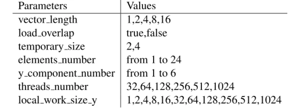
In order to try our approach, we took a very simple example which is a kernel that computes the Laplacian of an image and for which we want to minimize the time to compute a pixel. Figure A.1 shows the BOAST code to generate a Laplacian kernel. Figure A.2 shows one such generated kernel. This BOAST code was already implemented by the BOAST developers but as we will see finding the right parameter values was quite a challenge. There are multiple optimization that can be done to enhance the performance of this kernel each one of them are expressed by a parameter and its possible values. The parameters and their values we used to tune this applications are the following:
Parameters Values
vector length 1,2,4,8,16
load overlap true,false
temporary size 2,4
elements number from 1 to 24
y component number from 1 to 6
threads number 32,64,128,256,512,1024
local work size y 1,2,4,8,16,32,64,128,256,512,1024
1. Vector length allows to specify the size of the vectors used to performs the computation. The Laplacian can be easily vectorized and on hardware that provides vector support it allows to save some decoding phase as the same instruction is applied to the entire vector. As each architecture have different vector sizes, and some do not provide vector support we need to try the different values of vector size. Thus we try all the different vector size supported by OpenCL. Nvidia GPUs do not provide any vector support and vector variables are handle like scalar variable. However this can have a good effect on the caching but it can also has negative effect because it would increase data movement. Thus it is difficult to envision a model for this factor and considering it has a linear impact is a reasonable starting point.
2. Load overlap is related to the vectorization. As vectors are manipulated, when loading, some data overlap. Thus it is possible to synthetize the load from other data and conse-quently reduce the number of loads. As it is a factor with only 2 levels (true or false) the model for its impact is necessarily linear.
3. Temporary size allows to specify the size of the variables used to store intermediary results. Using smaller type can reduce the pressure on the registers but casting variables can also be harmful. Hence the default size is int (4) and we can also use short (2). Like load overlap it is a 2 levels factor hence we use a linear model for it.
4. Elements number splits the image into pieces of the size of elements number. This spec-ifies the of component (RGB) a threads will process. That is the amount of work per thread, as a consequence it defines the number of threads used to perform the computa-tion. Using more threads allows to compute more component in parallel. However it can also lead to a less efficient sharing of the cache resources as it will increase the number of memory loads. Also the higher the number of threads the more important the overhead due to their management. Hence the impact of the number of elements may be modeled as follow:
elements number+ 1
elements number
5. Y component number is used to specify how the work for a thread is organized by spec-ifying the tiling. It gives how the components of the image are distributed in the y-axis. This tilling optimization may take advantage of the organization of memory banks on Nvidia GPUs and thus improve the data usage. The impact is suspected to have an al-most quadratic shape and we can try either a model like this:
ycomponent number+ y component number2
Or either like this:
y component number+ 1
y component number
6. In OpenCL and Cuda, threads are grouped and scheduled by blocks on a compute unit. Which means that threads are not scheduled individually but by blocks. Threads number specifies the size of a group. Threads in a group can share data, bigger groups can lead to
better data usage. However smaller groups generally gives more scheduling opportunity but there might be an overhead due to a higher number of work groups to manage. We can either try this model:
threads number+ threads number2
Or this one:
threads number+ 1
threads number
7. Local work size y (lws y) determines how the threads are organized in a block and rep-resents the number of threads in the y-axis. For this parameter it is difficult to envision what kind of impact it can have so we started with a simple linear model.
The model we will consider are sums with at most level 2 interactions of the previous one. All the combinations of these parameters would gives a search space of 190080 points. However some points are unfeasible. For instance, having more component numbers in the y-axis (y component number) than number of component (elements number) itself makes no sense. We also have constraint the size of the kernel because it is limited to the available resources on the device. Exceeding the resources cause the kernel to crash. That is why use constraints to reject all the combinations that would produce a too big kernel or that is not correct. Finally it remains 23120 points in the search space. For comparison purpose we performed an exhaustive search which took about 154 hours.
The experiments are run on one machine with GPU Nvidia K40c using the driver 340.32 and two CPUs Intel E5-2630. The OS is Debian and we used the GCC compiler version 4.8.3. All the details about each experiments environment are available in the git repository.
4.3
Controlling measurement
Current hardware has became more and more complex and provides features such as power saving, frequency scaling, etc. . . Thus it is possible to have measurements that are different from an experiment to another even if the set of inputs is exactly the same. For instance, frequency scaling mechanism could chose to scale down the frequency of the CPU because the temperature inside the computer case has increased which would have an impact on the compute time. To have trusted measurements we are concerned about those kind of problems because the metric in our case, which is the time to compute a pixel, is sensitive to this. Thus we have to be protected against variability between the same measurements and especially the warm-up effect. This phenomena can occurs on devices providing energy saving features. This kind of devices generally have a performance mode and an idle mode. As long as the device does not have a lot of work it stays in idle mode but at a some threshold it switches to the performance mode. Thus the device does not provides all its capabilities immediately, hence the warm-up effect.
The measurement process is made as follow: 1. Generation of the next a version of the code
2. Compilation
3. Bench-marking on several image sizes multiple times.
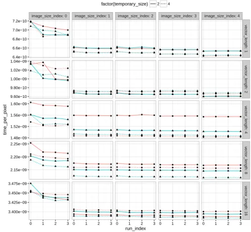
As the code is executed on a GPU, the latter has no work to do during the code generation and compilation phases. For this reason we suspected that warm-up effect can occurs at this moment and also after an image is loaded. We tried to see if on the GPU Nvidia K40 this effect is present. We also tried to quantify it along with the variability we could have between the different runs of the same version of the code in order to protect against it. Figure 4.1, illustrates what we expected, there is a power saving mechanism on Nvidia K40 which turns the GPU into idle mode when the computational intensity is bellow a threshold. This effect occurs on the first size of image tested, which is just after the code generation and compilation phases. The more run are performed the better the performances. It also could have been the case when going from one image size to another, the GPU could have switched to idle mode while the loading of the image, but is not the case. The GPU does not have the time to switch to idle mode. So to be protected against the warm-up effect we only need to make at least four runs on the first size of image and we keep the run that gives minimal time to compute one pixel. However we also did the same for all the size of images.
image_size_index: 0 image_size_index: 1 image_size_index: 2 image_size_index: 3 image_size_index: 4 ● ● ● ● ● ● ● ● ● ● ● ● ● ● ● ● ● ● ● ● ● ● ● ● ● ● ● ● ● ● ● ● ● ● ● ● ● ● ● ● ● ● ● ● ● ● ● ● ● ● ● ● ● ● ● ● ● ● ● ● ● ● ● ● ● ● ● ● ● ● ● ● ● ● ● ● ● ● ● ● ● ● ● ● ● ● ● ● ● ● ● ● ● ● ● ● ● ● ● ● ● ● ● ● ● ● ● ● ● ● ● ● ● ● ● ● ● ● ● ● ● ● ● ● ● ● ● ● ● ● ● ● ● ● ● ● ● ● ● ● ● ● ● ● ● ● ● ● ● ● ● ● ● ● ● ● ● ● ● ● ● ● ● ● ● ● ● ● ● ● ● ● ● ● ● ● ● ● ● ● ● ● ● ● ● ● ● ● ● ● ● ● ● ● ● ● ● ● ● ● 6.4e−10 6.6e−10 6.8e−10 7.0e−10 7.2e−10 9.60e−10 9.80e−10 1.00e−09 1.02e−09 1.04e−09 1.48e−09 1.52e−09 1.56e−09 1.60e−09 2.15e−09 2.20e−09 2.25e−09 3.400e−09 3.425e−09 3.450e−09 3.475e−09 v ector_length: 1 v ector_length: 2 v ector_length: 4 v ector_length: 8 v ector_length: 16 0 1 2 3 0 1 2 3 0 1 2 3 0 1 2 3 0 1 2 3 run_index time_per_pix el
factor(load_overlap) ● false true
factor(temporary_size) 2 4
Figure 4.1 – Warm-up effect: This figure presents the time to compute a pixel on 4 different runs for 5 different image sizes and for different vector lengths. We can see that in the first image size we have some variability and the time to compute a pixel dicrease when the run index increase while for the other image size the performances are stable. The first image size being the first one tested just after the compilation of the kernel. This assess the presence of a warm-up effect on Nvidia GPUs.
5
Envisioned general approach
When using fully automated tools, the user has no feedback about the optimization process and does not have a lot of control. How good is the optimized version of the code? How is it possible to improve it? What does the search space look like? What are the parameters that have a big impact (high-order parameters) and those which have a small impact (low-order parameters)? All these questions are necessary to understand the structure of the problem and provide valuable information to the expert to be able to prune the search space correctly and to choose the most suited search techniques. Thus we investigated the design of a semi-automated approach where the user tunes his application in an interactive way. All along the tuning process, this method provides valuable information to the user to guide him and exploit his knowledge. Of course, this assumes that the application developer understands well his kernel and knows the reason each code optimization he used.
As the objective the function is empirical and is costly to evaluate, our approach consists in sampling the search space with only few points to build a model in order to approximate it at low cost. We focused on linear regression because usually, it is enough to model accurately computer phenomenon. However a correct modeling goes to together with efficient sampling techniques. That is why we used techniques inspired from design of experiments where the goal is to maximize the amount of information and minimize the number of points.
The Figure 5.1 shows the workflow of our approach:
1. The search space is sampled by taking into account the objective of the user. For instance if the user wants to have a first overview of the high-order parameters or if he wants to refine his model or if he needs to obtain more information about a precise part of the search space.
2. Using linear regression, a model is built based on the hypothesis about the kernel perfor-mances provided by the user. This step allows the developer to test multiple hypothesis, by trying different models and keeping the most suited. This allows to determine what are the parameters that have the most impact. Parameters that have less impact are removed from the model and will be re-injected later when higher order parameters are fixed. It also allows to estimate what kind of impact they have by finding their coefficients. If the user is not satisfied about the result of the linear regression he can ask additional points. 3. Once the user has found a satisfying model, this latter is instantiated in order to predict
the best values only for the relevant parameters.
5. The remaining parameters are re-injected in the tuning process which iterates until all the wanted parameters are fixed.
6. At the end the user has either the best estimated solution or at least the most interesting region of the search space.
In short the tuning is done through an iterative and instrumented process where the user refines his model according to the extracted information.
1. Sample the search space : Taking into account the
user's need
2. Linear regression :
• Find relevant parameters • Refine the model by
checking hypothesis 3. Instantiation : Predict best values of significant parameters
4. Pruning the search : Fixing these parameters
5. Re-inject unused parameters 6. Best estimated solution or region Feedback Propose models User
Figure 5.1 – Semi-automatic approach workflow. This Figure shows how linear regression techniques are combined with design of experiments techniques.
6
Results
To evaluate our solution, we compared it against the following search methods that are gener-ally used in auto-tuning literature using an exploration budget of 120 points (0.5% of the search space) that must not be exceeded:
• RS: is the uniform random search that takes points randomly in the search space with equal probabilities.
• LHS: it is a not a method used to search, it is a sampling technique which takes points randomly but which also maximizes the distance between them to cover the full search space. However we wanted to see how a search method based on it, would perform. • GS (Greedy Search): we implemented a greedy search which is a derivative-free local
search. From a random starting point, this algorithm explores all the possible directions at distance one and moves to the direction that leads to the best improvement. This kind of algorithm is efficient on convex objective function but can easily be trapped in local optimum. In such case, the algorithm may not have used its whole experimental budget. This is why to illustrate the geometry of the search space through the performance of this algorithm, we consider a variant of this algorithm, GSR (Greedy Search with Restart), that will repeatedly pick another point uniformly chosen at random (i.e., like the RS strat-egy) and perform greedy local improvements until the maximum number of experiments is reached. The best solution found so far is then returned.
• GA: BOAST embeds an implementation of a genetic algorithm. We used a population size of 20 and mutation rate of 0.1. Among the different configurations tested, it was the one that gave the best results but it may be possible to obtain better results by tuning further the genetic algorithm parameters.
Although the linear regression of the mean is the classical tool to use in combination with design of experiments, while performing our study, we realized some of the underlying hypoth-esis (in particular the uniformity of variance1) did not hold and that using instead a technique called quantile regression may be more sound. We therefore report both approaches and will explain later in more details their difference:
• LM: this corresponds to the iterative approach described in the previous section and relying on a classical linear model using least square regression which allows to estimate the expectation of performance. A first sample of the whole space (with slightly less thant half of the experimental budget) is done and several models are evaluated. The best and simpler ones are kept and used to fix the corresponding parameters. The approach is repeated on the restricted space. If there are no more clear directions suggested by the model and a few more experiments can be done, a small sampling of the restricted set is carried out and the best solution is returned.
• RQ: this approach is similar to the previous one but relies on quantile regression instead and tries to model how the 5% smallest values depend on the various input parameters. We measured each methods 1000 times. The average time needed to perform a single exploration (120 points) is approximately 43 minutes. Since we wanted to compare our method to the absolute best solution, we have also measured the whole space, which takes about 144 hours. For each algorithm, we have evaluated the slowdown achieved compared to the best solution available in the entire search space.
Our approach is intended to be semi-automatic but for evaluation purpose we automated the process. Based on few observations we made by trying the full model and eliminating useless parameters on different random sets of points, we found out that the parameters which have a significant impact at each step of the tuning process are generally the same. For this reason we decided to apply exactly the same strategy each time without considering the random set:
1. Sampling 50 points at random
2. Setting vector length and lws y and pruning the search space using the model: time per pixel= vector length + lws y
3. Sampling 40 additional points at random in the pruned search space
4. Setting the factor y component number and pruning the search space using the model:
time per pixel= y component number
5. Sampling 20 additional points at random in the pruned search space
6. Setting the factor elements number and pruning the search space using the model: time per pixel= elements number
7. Sampling 5 additional points at random in the pruned search space
8. Setting the factor threads number and pruning the search space using the model:
time per pixel= threads number + 1
threads number
9. At this step, after pruning, only 4 points remain in the search space. As we are below (119 points) the maximum number of points (120 points), we take the best remaining combination of these 4 points.
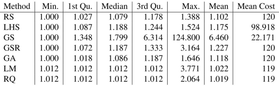
Table 6.1 – This table shows the minimum, first quartile, median, mean, third quartile and maximum slowdown including the mean number of points used by each method.
Method Min. 1st Qu. Median 3rd Qu. Max. Mean Mean Cost
RS 1.000 1.027 1.079 1.178 1.388 1.102 120 LHS 1.000 1.087 1.188 1.244 1.524 1.175 98.918 GS 1.000 1.348 1.799 6.314 124.800 6.460 22.171 GSR 1.000 1.072 1.187 1.333 3.164 1.227 120 GA 1.000 1.018 1.086 1.187 1.646 1.118 120 LM 1.012 1.012 1.012 1.012 3.771 1.022 119 RQ 1.012 1.012 1.012 1.012 2.064 1.019 119
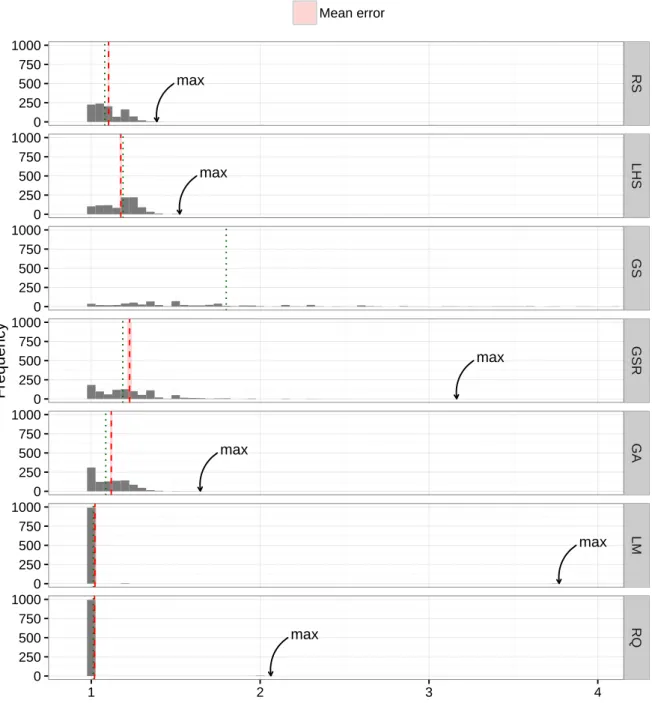
Figure 6.1 shows the results of the different methods. Let us start with methods that do not exploit the geometry of the space. The first observation that can be made is that the uniform random search RS is quite efficient. Half of the time we get a slowdown that is less than 7.9% and we do not get a maximum slowdown that is higher than 38.8%. A likely explanation of the efficiency of the random search will be given later. Surprisingly, the LHS approach did not improve at all over RS since the expected slowdown increases from 10.2% to 17.5% (see Table 6.1). We do not have a convincing explanation for this phenomenon.
Now, let us focus on strategies that build on local search. The GS strategy is extremely inefficient since almost half of the time we get a slowdown of higher than 2. It can be every far from the optimal solution (up to 125 slower as reported in Table 6.1), which is why only a few solutions are reported in the histograms of Figure 6.1. where we restrict to slowdowns smaller than 3. The average number of configurations explored by this greedy approach is also very low (about 22 in average), which shows that our search space is riddled with local minima. In this context, combining several starting points in the GSR really makes it appears like a mix between RS and GS and greatly improves upon GS. The worst solution is never slower than a factor of 3.164 and half of the time the slowdown is below 18.7%. Still, this remains worse than the simple Random Sampling strategy and shows that locality is of very little use.
Now let us consider the GA that is a technique, which is known to seamlessly handle local minimum as it is a specific form of simulated annealing. Unfortunately, this generic technique does not really improves upon the simple RS since the slowdown is less than 8.6% half of the time (resp. 7.9% for a RS), the mean slowdown is 11.8% (resp. 10.2% for a RS) and a maximum slowdown of 64.6% (resp 38.8% for a RS). Again, exploiting locality is quite difficult. It is possible that much better solutions could be obtained with more experiments but these experiments tend to disqualify the GA approach in a tight experimental budget.
Finally, the results based on the global modeling approach lead to surprisingly good results since most executions lead to a solution that is only 1.2% away from the optimal solution. This is explained by the fact that a few samples are sufficient to detect trends and how several parameters should be fixed and thus guide the analyst toward the right region. The subsequent sampling allows to fix the remaining parameters and to find good solution in all cases. However in only 3 cases LM does worst than the worst case of GA (resp. 1.646) with slowdown of 3.77 (see Table 6.1). RQ managed to have a worst case better than LM with a slowdown of 2.064 but still higher than GA.
In brief, the regression of expectation gives almost every time the exactly same results which is very close to the best solution of the entire search space but it never reaches it. With
the quantile regression we managed to improve the worst solution but we could not improve the best solution return by LM. However both LM and RQ very rarely gives worse solutions than GA or RS.
max max max max max max 0 250 500 750 1000 0 250 500 750 1000 0 250 500 750 1000 0 250 500 750 1000 0 250 500 750 1000 0 250 500 750 1000 0 250 500 750 1000 RS LHS GS GSR GA LM RQ 1 2 3 4
Slowdown compared to the optimal solution
Frequency
Mean error
Figure 6.1 – Comparison of the efficiency of the different search methods. The histogram of the slowdown (1000 values for each method) allows to better compare the different heuristics. The red dashed line depicts the estimation of the mean with the corresponding 95% confidence in-terval in gray. The green dotted line depicts the sample median. The arrows show the maximum values, expect for GS which is out of the range.
7
Analysis
This part gives a study of the search space and an explanation of the results of our approach. We also explain why the quantile regression is more suited than regression of expectation in optimization purpose. In order to perform our experiment we automatized our approach by blindly using the same model and the same pruning strategy without considering the working set of points. This gives us an overview of how it could perform but it is not intended to use like this. Hence this part explains the case where the prediction is made correctly and when it fails.
7.1
Characteristics of the search space
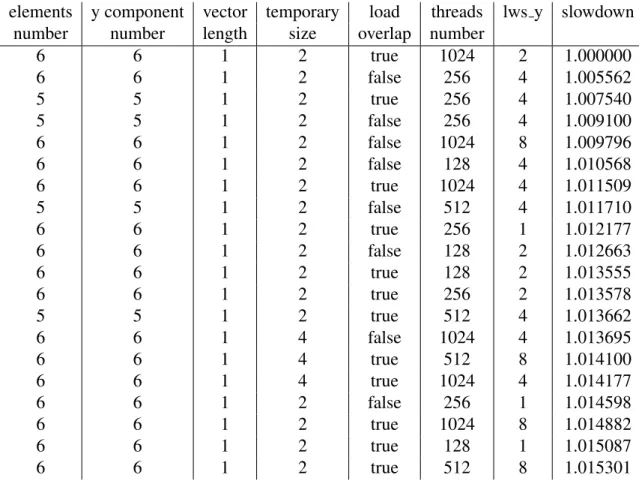
By studying the characteristics of the search space we can understand the structure of the prob-lem in order to be able to understand the results of the different search techniques. Figure 7.1 and Table 7.1 show the distribution of the combinations over the search space in term of slow-down. This search space contains a lot of good combinations, half of them have a slowdown that is less x6.1 which is x2.8 faster than the mean slowdown. However there are few bad ones with the worst at a slowdown of x382. Thus the probability of finding a good performing combination is high, this is the reason why randomized algorithms such as the RS, GA and LHS obtains results good. Among the 23120 combinations there are 170 which have a slow-down lower than 10%. In order to get less than this slowslow-down with a probability of 0.9 with the random search we would need to pick at least 312 points at random. And if we hope to get the same level of performance as with LM, we would need 6654 points at least. Yet, this search space remains complicated, because as we saw previously our local search GS failed which means there are a lot of local optimum in which it is stuck and some are far from the optimal one. The Table 7.2 shows the best 20 combinations, they are very similar, they all have a vector length of size 1 and a number of elements and a y component number of 5 or 6. Which means that they are very located but there are still some local optimum in this area because if we try to run the GS on the best solution of LM, it did not make any progress.
We can also notice in the Figure 7.2 that the variability is not the same everywhere, hence our data are heteroscedastics. This is because the noise does not follow the same law for the different value of the same parameters. This noise is due to complex interactions between parameters.
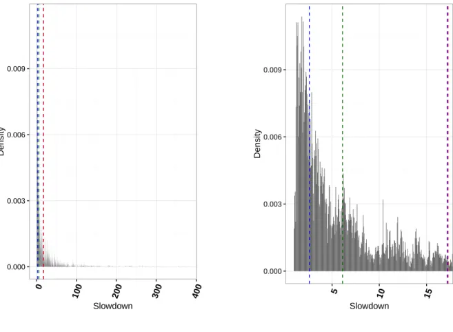
0.000 0.003 0.006 0.009 0 100 200 300 400 Slowdown Density
(a) Global search space
0.000 0.003 0.006 0.009 5 10 15 Slowdown Density
(b) Zoomed search space
Figure 7.1 – These figures present the slowdown of the combination of the entire search space. The Figure (a) is a global view and the Figure (b) focuses on combination between a slowdown of 0 and 20. The red dotted line represents the mean, the green one the median, the blue one on the left the 1st. quartile and the blue one on the right the 3rd. quartile.
Table 7.1 – This table presents the slowdown characteristics of the search space
Min 1st Q. Median Mean 3rd Q. Max
1.00 2.599 6.116 17.276 17.177 382.168
7.2
Differences between regression of expectation
and quantile regression
The previous results showed that using linear regression gives often good results. But there is a slight difference between regression of expectation and quantile regression. It is due to the fact that they do not predict the same thing.
Linear regression of expectation has already been used successfully with auto-tuning prob-lems by Brewer in the 1990s[6]. But this method have been put aside for no real reasons to our knowledge. Using this method to study the impact of the parameters with using linear mod-els to approximate the behavior of the search space coupled with efficient sampling strategies
Table 7.2 – This table presents the top 20 of the best combinations
elements y component vector temporary load threads lws y slowdown
number number length size overlap number
6 6 1 2 true 1024 2 1.000000 6 6 1 2 false 256 4 1.005562 5 5 1 2 true 256 4 1.007540 5 5 1 2 false 256 4 1.009100 6 6 1 2 false 1024 8 1.009796 6 6 1 2 false 128 4 1.010568 6 6 1 2 true 1024 4 1.011509 5 5 1 2 false 512 4 1.011710 6 6 1 2 true 256 1 1.012177 6 6 1 2 false 128 2 1.012663 6 6 1 2 true 128 2 1.013555 6 6 1 2 true 256 2 1.013578 5 5 1 2 true 512 4 1.013662 6 6 1 4 false 1024 4 1.013695 6 6 1 4 true 512 8 1.014100 6 6 1 4 true 1024 4 1.014177 6 6 1 2 false 256 1 1.014598 6 6 1 2 true 1024 8 1.014882 6 6 1 2 true 128 1 1.015087 6 6 1 2 true 512 8 1.015301
seemed very appealing to us.
This techniques assumes that the noise is uniform and more specifically follows the Gaus-sian law, in this case we say that the variable are homoscedastics. However the Figures 7.3a and 7.3b show that in the case of our Laplacian kernel, which is a very simple case, we have heteroscedasticity, which means that the noise is non-uniform because it is due to complex in-teraction between parameters. Heteroscedasticity is problematic because the least square is not the Best Linear Unbiased Estimator in this case and it biases the standard errors and thus the co-efficient of determination which makes it more difficult to evaluate the accuracy of the model. In addition, we want to predict the minimum value of the objective function not the mean. With non-uniform noise, the evolution of the minimum value does not follow the evolution of the mean (see Figure 7.3b).
If the error law is the same everywhere as in the left in Figure 7.3a we can still have the minimum values that follow the same evolution as the mean and we can still predict the mini-mum. The resulting model and approximation can still be correct and we can easily know what is the best size of vector. But we would still need to make assumptions that about the error and we do not know anything about it. In the Figure 7.3b, the evolution of the mean and the evolution of the minimum are not correlated and the best value is not predicted correctly.
We conclude that in the case of heteroscedasticity and non-uniform error law, linear re-gression tracks the general tendency of impact of the parameters. But in our case in which we are interested about the minimum which is uncorrelated to the mean, the linear regression of expectation cannot lead to the global optimum and we need another estimator for the minimum.
5.0e−10 1.0e−09 1.5e−09 2.0e−09 2.5e−09 4 8 12 16 Vector length
Time per pix
el in seconds
Impact of the vector length
5.0e−10 1.0e−09 1.5e−09 2.0e−09 2.5e−09 4 8 12 16 X component number
Time per pix
el in seconds
Impact of number of component on the x−axis
Figure 7.2 – Non-uniform variance: This figures that shows in our data, the noise does not have the same law everywhere.
Quantile regression gives the estimate of quantile and has been proven successful in the ecologic field[7] where complex interactions between factors lead to non-uniform noise which is exactly the case of our Laplacian kernel. Moreover it has the ability to estimate multiple ten-dency from the minimum to the maximum. As we want to minimize the time to compute a pixel we need to estimate the minimum and regression on the 5th percentile is a generally a good es-timation of it[12]. Figure 7.3 illustrates the comparison between regression of expectation and quantile regression. The regression of expectation estimates that the best performing version has a x component number of 4 which is not true. While the quantile regression of the 5th percentile succeed in predicting that the best performing version has a x component number of 1. So the regression of expectation may not find the minimum while the quantile regression does if the model is correct. That is probably one of the reason why the worst case of RQ is better than the worst case of LM.
7.3
LM: Success and ”failures”
To study in more detailed the results of our approach, we took the worst and the best solutions to understand why sometimes it fails to converge to the same value and how a correct and an incorrect optimization process looks like.
The worst solution failed in the first stage of the optimization process (see Table 7.3). In-deed, vector length and lws y are the first factors we fixed in our strategy. It predicted a good value for lws y, but instead of predicting that the best size of vector is 1, the model predicted a size of 16 which is the worst value. There are several hints that gives indications about the quality of the prediction.
First, the coefficient of determination tells us about the fit of a model, the closer to 1, the better the model explains the variance. However when comparing models this is not sufficient.
Table 7.3 – This table presents the worst solution of LM
elements y component vector temporary load threads lws y slowdown
number number length size overlap number
24 6 16 2 false 64 1 3.771183
It is possible to have an acceptable R-squared with a too high uncertainty on the coefficients, e.g. by over-fitting, this will gives a bad prediction.
The p-values give information about the importance of a factor in the objective function, this gives us clues about the structure of the search space. The closer to zero, the bigger the impact, thus we only keep factors for which the p-values is lower than 0.001.It is important to go from high order factors to low order factors in order to refine the model properly. Trying to fix a factor that has a small impact too early would lead to a premature pruning of the search and as a results lots of good combinations would be missed.
Then the order of magnitude of the standard error compared to estimate of the coeffi-cients has to be taken into consideration. The coefficoeffi-cients gives the slope which indicates what kind of impact the factor has. For example, in our case vector length has a linear impact, a positive coefficient means the lower vector length is the lower the time to compute a pixel. Comparing the coefficients with the standard errors gives information about the uncertainty in the estimate of the coefficient, the bigger the standard error compared to the coefficient, the more inaccurate the prediction.
An additional way of assessing the quality of a model is to compare the predicted values with the real ones, the more they are correlated the more accurate the model. The most impor-tant is correlation between the low values as we are interested mostly by the minimum values.
All these information allow us to compare different models and evaluate the quality of the prediction. The Table 7.4 shows the results of fitting the model bellow in the worst case:
vectorlength+ lwsy
First, with this set of points, the factor vector length was not significant enough and was fixed prematurely. Second, the standard error is equal to 5.953e-11 and the estimate is equal to -2.316e-11, the standard error is too big compared to the estimate. Which means that the coefficient is between -8.269e-11 and 3.637e-11. Thus we do not know if the coefficient is positive or negative, hence we do not know if the best value for vector length should be the smallest or the biggest possible. The Figure 7.4a shows the prediction against the real values, good predicted values are not that good and some can be very bad. This kind of situations can be detected easily by the user and thus he can take correct decision. The explanation of why this worst case happened is because our automated experiment process did not make the previous analysis and applied the same strategy whether the model is correct or not.
Table 7.4 – This table presents the fit of an incorrect model
Coef Std. err. p-values
vector length -2.316 (-11) 5.953 (-11) 0.69904
lws y 5.572 (-12) 1.625 (-12) 0.00127
The good case happens when our strategy is applied like we expected. When using the model vector length + lws y the fit is acceptable with a coefficient of determination of 0.5431.