Modeling of the effect of a thermoelectric magnetic force onto conducting particles immersed in the liquid metal

(1)

HAL Id: hal-01232204

https://hal-amu.archives-ouvertes.fr/hal-01232204

Submitted on 23 Nov 2015

HAL is a multi-disciplinary open access archive for the deposit and dissemination of sci-entific research documents, whether they are pub-lished or not. The documents may come from teaching and research institutions in France or abroad, or from public or private research centers.

L’archive ouverte pluridisciplinaire HAL, est destinée au dépôt et à la diffusion de documents scientifiques de niveau recherche, publiés ou non, émanant des établissements d’enseignement et de recherche français ou étrangers, des laboratoires publics ou privés.

Modeling of the effect of a thermoelectric magnetic force

onto conducting particles immersed in the liquid metal

y Du Terrail Couvat, O Budenkova, A Gagnoud, G. Salloum Abou Jaoude, H

Nguyen-Thi, G Reinhart, J Wang, Z-M Ren, Y Fautrelle

To cite this version:

y Du Terrail Couvat, O Budenkova, A Gagnoud, G. Salloum Abou Jaoude, H Nguyen-Thi, et al.. Modeling of the effect of a thermoelectric magnetic force onto conducting particles immersed in the liquid metal. IOP Conference Series: Materials Science and Engineering, IOP Publishing, 2015, 84 (012019), �10.1088/1757-899x/84/1/012019�. �hal-01232204�

(2)

This content has been downloaded from IOPscience. Please scroll down to see the full text.

Download details:

IP Address: 147.94.212.92

This content was downloaded on 23/11/2015 at 09:59

Please note that terms and conditions apply.

Modeling of the effect of a thermoelectric magnetic force onto conducting particles immersed

in the liquid metal

View the table of contents for this issue, or go to the journal homepage for more 2015 IOP Conf. Ser.: Mater. Sci. Eng. 84 012019

(http://iopscience.iop.org/1757-899X/84/1/012019)

(3)

Modeling of the effect of a thermoelectric magnetic force onto

conducting particles immersed in the liquid metal

Y Du Terrail Couvat1,2_{, O Budenkova}1,2,6_{, A Gagnoud}1,2_{, G. Salloum Abou}

Jaoude3,4_{, H Nguyen-Thi}3,4_{, G Reinhart}3,4_{, J Wang}5_{, Z-M Ren}5_and

Y Fautrelle1,2

1_{CNRS, SIMAP, UMR 5266 Grenoble, France} 2_{SIMAP, Grenoble Institute of Technology, France} 3_{IM2NP, Aix-Marseille and Toulon University, France} 4_{CNRS, IM2NP, UMR 7334, Aix-Marseille, France}

5_{Department of Materials Sciences, Shanghai University, China}

Abstract. Simulation of a thermo-electromagnetic force which acts on a conducting particle

immersed into liquid metal is performed using multi-gird multi-physics software AEQUATIO. To verify numerical solutions a model thermoelectric problem is solved using two methods. In the first one a phase function is used to indicate the phase transition whereas in the second the solid particle is described with a real frontier of a simplified shape. Numerical and analytical solutions for a model problem qualitatively agree but strong oscillations are observed in a numerical solution with a phase function. Further AEQUQTIO is applied for calculation of the velocity of a dendrite fragment observed in-situ in experiment of solidification of AlCu alloy. Numerical solution gives a good agreement with the experimental observation.

1. Introduction

Electromagnetic fields are used in metallurgical processes since several decades. Traditionally, static magnetic fields are applied to suppress the liquid motion in the bulk liquid due to the braking effect of the Lorentz force. The latter is a result of interaction between the electric current, induced by a moving liquid, and the imposed magnetic field. Yet, during solidification processes bulk materials are subjected to temperature gradients and thermo-physical properties of materials can change abruptly because of phase transition. This leads to appearance of a thermoelectric current near the liquid-solid interface and further to the thermoelectric magnetic force (TEMF) which is a result of interaction between the thermoelectric current and the applied magnetic field. Theoretical studies of the effect of TEMF force on the convective flows were made several decades ago [1] and experimental evidences were first found in crystal growth [2-3]. Post-mortem analysis of samples of alloys solidified under the action of static magnetic field showed remarkable results [4]. Nowadays, advanced in-situ observations made with X-rays allow one to identify the effect of external fields in real time [5-6]. However, despite diverse experimental results, very limited number of numerical simulations can be cited and most of them are applied either for a very small calculation domain [7] or for simple geometries [8]. This is related to the fact that an intensive thermoelectric current appears in a very thin layer in the bulk liquid near the solid-liquid interface and a fine calculation mesh is required to capture this. On the other hand, the effect of the thermoelectric magnetic force spreads over large distance in a

6

To whom any correspondence should be addressed at [email protected]

MCWASP IOP Publishing

IOP Conf. Series: Materials Science and Engineering 84 (2015) 012019 doi:10.1088/1757-899X/84/1/012019

Content from this work may be used under the terms of theCreative Commons Attribution 3.0 licence. Any further distribution of this work must maintain attribution to the author(s) and the title of the work, journal citation and DOI.

(4)

form of convection and transport of the solid phase in the liquid, as strains and deformation of the solidified structure. Therefore, to study numerically the effect of the TEMF in solidification of alloys one needs either to use an average approach which would account lower-scale information at macro-scale or to employ a multi-grid technique in order to link processes at micromacro-scale and at macromacro-scale in a direct way.

A numerical toolbox AEQUATIO is intended for use of multiple grids in a calculation domain and couples solutions obtained at different scales. The present work was inspired by the idea of modeling of a particular phenomenon observed in the experiment on solidification of Al-4wt%Cu alloy which is briefly described in the next section. Mathematical statement of the problem and numerical approach are presented in sections 3 and 4. Then comparisons between the analytical and numerical results for a model problem are made and results of simulation are compared with experimental observations. 2. Experimental observation

In the experiment performed with in-situ X-ray observation at ESRF a liquid Al-4wt%Cu alloy was solidified from the bottom in a crucible 6mm×40mm×0.2mm. A scheme of the set-up is shown in figure 1. A static magnetic field was generated by a permanent magnet fixed close to the crucible.

Figure 1. Geometry for the experiment on solidification of Al-4wt%Cu performed at ESRF, G=3000 K/m and B=0.08T [9].

Figure 2. Registered detachment of dendrite pieces and their motion in horizontal direction, time interval between the frames (a)-(b) and (b)-(c) is 1.4s. Frame (d) shows detachment of a larger fragment [9].

In the experiment several events of detachment of dendrite pieces were observed. A sequence of frames which shows motion of detached pieces in the horizontal direction is given in figure 2. Since this effect was not observed in experiments without magnetic field, there are strong grounds to believe that thermoelectric magnetic force acting on the solid phase is at the origin of this phenomenon. Image treatment showed that the average velocity of the motion of a dendrite fragment depends on its size and is about 130-200µm/s [9].

3. Statement of the problem

Below mathematical formulations for two problems are given. The first one is related to the case of the experiment whereas the second concerns a model thermoelectric problem which we used to verify numerical results obtained with AEQUATIO.

3.1. Statement of the problem for the experimental case

The system of equations to be solved for each phase includes stationary equation for the energy transfer, continuity equation for the electric current and relation between the density of the electric current and temperature gradient:

(

∇

)

=0

∇

λ

i Ti (1)

(5)

0 = ∇ji ! (2)

!j_i=−

σ

_i∇U_i −

σ

_iS_i∇T_i (3)

In (1-3) the index i=S,L is related either to the solid or to the liquid phase and U is an electric potential, which, in fact, should be found. Notations for other variables and their values for the Al-4wt%Cu alloy are given in the table 1. The boundary conditions for the temperature are fixed temperature values at the top and bottom of the calculation domain and no heat flux through the lateral boundaries:

T _z₌_z_min=T₁ (4a) T _z₌_z_max=T₂ (4b) 0 = ⋅ ∇T n!_wall (4c)

For the current we presume insulating conditions for all surfaces bounded the calculation domain: 0 = ⋅ _wall i n j ! ! (5)

At the solid-liquid interface conditions of continuity of heat fluxes and normal component should be satisfied that gives following conditions for the temperature and electric potential, respectively:

SL L L SL S S∇T ⋅n! =λ ∇T ⋅n! λ (6)

(

σS∇US +σSSS∇TS

)

⋅n!_SL=

(

σL∇UL +σLSL∇TL

)

⋅n!_SL (7)

The thermoelectric magnetic force (per unit volume) acting in each phase is given as

B j =

f!_TEM,_i !_i× ! (8)

The velocity and the trajectory of the particle can be found from Newton’s equation:

Stokes S TEM S ₌_F _F dt V d ! ! ! − , ρτ

(9)

where τ is the volume of the particle and the TEMF acting onto the whole particle is

∫

= τ τ d f F!_TEM_,_S !_TEM_,_S (10)

Stokes’ drag force is taken proportional to the velocity of the particle and to the viscosity of the solid:

F!_Stokes =A⋅V!_S (11)

where coefficient A depends on the particle geometry. If the thermoelectric magnetic force does not change with particle motion, then the analytical solution of (9) is given as

⎥ ⎦ ⎤ ⎢ ⎣ ⎡ ⎟⎟⎠ ⎞ ⎜⎜⎝ ⎛₋ − = A t A F V_S TEM S ρτ exp 1 , ! ! (12)

3.2. Statement of a model problem

A simple thermoelectric problem which allows analytical solution for the system of equation (1)-(3) is a conducting solid sphere immersed into a conducting infinite media. The boundary conditions

(4a)-MCWASP IOP Publishing

(6)

(4c) and (5) are replaced with a constant one-dimensional temperature gradient and zero electric current at infinity. Let us suppose that the thermal gradient G in infinity is directed along the z -axis.

Then the analytical solution for the problem shows that the thermoelectric current in the whole domain circulates in the plane (z,y) with the maximal density in the solid particle and decays with a third power of a distance in the bulk liquid [10]. If a uniform static magnetic field acts in the x direction as

x

i B

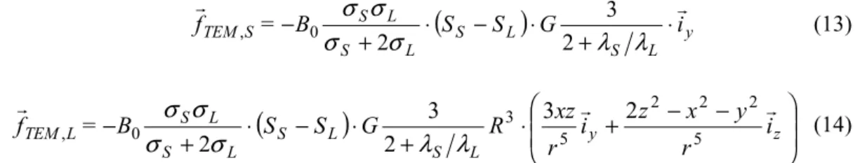
B!= ₀! , then the analytical solution for the thermoelectric force acting in the liquid and in the solid calculated using (8) and presented in Cartesian coordinates system with the origin at the centre of the sphere has the following form:

(

)

y L S L S L S L S S TEM = B S S G i f! ⋅! + ⋅ − ⋅ + − λ λ σ σ σ σ 2 3 2 0 , (13)

(

)

_⎟⎟ ⎠ ⎞ ⎜ ⎜ ⎝ ⎛ ₋ ₋ + ⋅ + ⋅ − ⋅ + − y z L S L S L S L S L TEM i r y x z i r xz R G S S B = f ! ! ! 5 2 2 2 5 3 0 , _σσ σ₂_σ ₂ _λ3 _λ 3 2 (14)

Note that the force which acts onto particle f!_TEM_,_S is constant and is directed along the y-axis in a negative direction if a difference of Seebeck coefficient is positive and vice versa.

4. Numerical approach

AEQUATIO is a toolbox based on the finite elements methods [11]. The spatial discretization for partial differential equations is obtained with Galerkin method and one or several calculation meshes can be used in the domain. The solution is sought in the elements’ nodes and interpolation polynomials of Lagrange are of the second degree. In the present problem coupled equations for the energy and electric current (1)-(3) are projected over two meshes: the one which is constructed for the whole domain and which is coarse and a significantly finer mesh for a sub-domain around the particle (figure 3). The boundary conditions for the sub-domain are obtained via interpolation of data from the coarse mesh. We construct only one system of linear equations taking into account the two meshes.

a b

Figure 3. Illustration to the domain and sub-domain division in AEQUATIO toolbox. a: complete geometry of the problem with a calculation domain and sub-domain in its centre, particle inside the sub-domain seen as a point and b: sub-domain and the particle

The aim of the present work was to implement the thermoelectric magnetic equations into AEQUATIO toolbox using two different methods described below and to apply one of them for simulation of the experimental observation. The first method implied a straightforward utilization of a “phase function”

φ

(r!

)

which defines the properties of materials thus indicating transition between the

(7)

two phases but without using a sharp boundary between them. The second method is to describe a real frontier for a particle of simplified from, like, for example, cubic. Motivation for the use of phase function is driven by methods like volume of fluids or phase field where it is employed to calculate the evolution of the solid phase. One of advantages of implementation of phase function is that we can use a regular mesh in the sub-domain even if the particle has irregular form. Another advantage is that governing equations (1)-(5) can be solved in a unified manner without special treatment of the conditions at the solid-liquid interface.

5. Results and discussion

Results of numerical simulations presented below are given for points within the sub-domain containing the particle. Local values for the density of the electric current and for the thermoelectric magnetic force are calculated on a grid with obtained values in the mesh nodes handled with interpolations and derivation techniques used in finite elements method.

5.1. Comparison of the analytical solution and numerical results with phase function for a model problem

At the first step a comparison between the analytical solution and the ones obtained using AEQUTIO toolbox were made. In an analytic model a sphere of a diameter of 1 mm was taken, i.e.R=50µm is used in (11)-(14). To satisfy the condition of infinite media the size of the 3D computational domain in AEQUATIO simulations was taken 50 times larger than the sphere: 50×50×50 mm and was meshed with 4 elements in each direction. The phase function corresponded to a sphere, i.e. had a form

⎩ ⎨ ⎧ > ≤ = R r if R r if r _! ! ! 0 , 1 ) ( φ (15)

The size of a cubic sub-domain contained a spherical particle was four times larger than the particle: 4×4×4 mm. Every property γ for materials used in the calculations was presented as linear combination of the value for the solid γS and the liquid γL phase:

( )

r!

γ

_S

φ

r!

γ

_L

(

φ

( )

r!

)

γ

= ⋅ ( )+ ⋅1− (16)

We considered two combinations for the values of Seebeck coefficients in the liquid and in the solid phase. The first case with SS= −1·10-6 V/K and SL= −2·10-6 V/K corresponds to values measured for Sn-Pb alloy [12]. The difference SS−SL=1·10-6

V/K

is positive, and the TEMF acts along the y-axis in negative direction. In figure 4a we present distributions of the force along the line parallel to the z-axis which passes through the center of the sphere and lies within the sub-domain used in numerical simulations. The maximal value of the force is inside the particle for −0.5·10-3m≤z≤0.5·10-3_{m. Then} the TEMF decreases rapidly and almost disappears toward boundaries of the sub-domain which are at

m

3

10 1⋅ −

± . Surprisingly, in numerical simulations qualitatively correct results are obtained already if a sub-domain is meshed only with 5 elements in each direction, but the value of force is significantly higher than the one predicted theoretically. With increasing the number of cells in a sub-domain, numerical and analytical results become closer and for the sub-domain mesh containing 30 cells in each direction the maximal difference between the numerical and analytical solution is about 8%, yet oscillations appear in numerical solution.

Situation changes dramatically for other values of Seebeck coefficients which were measured for an Al-Cu alloy and are given in the table 1. In this case the difference SS−SL=−1.6·10-6

V/K

is negative and TEMF is co-directed with y-axis. The analytical model still predicts monotone behavior for the force with transition from the liquid to the solid phase, but in the numerical solution strong oscillations of the force is observed near the solid-liquid phase transition (figure 4b). Nevertheless, apart from two jumps the qualitative behavior of the numerical solution is not close to the analytical one. We suppose that oscillations in numerical solution are related to a discontinuity of the chosen

(8)

phase function and can be minimized if a smooth variation of physical properties with transition between the two phases is assured.

a b

Figure 4. Analytical and numerical solutions obtained in a model problem for the y-component of the thermoelectric force along the z-axis, origin of the coordinate system is at the centre of the sphere. The sphere in numerical solution is given with the phase function (15). a. SS−SL=1·10-6

V/K

and b: SS−SL=−1.6·10-6

V/K

, other properties are as in table 1.

5.2. Comparison of the analytical solution for a sphere and numerical results for a cubic particle with a real frontier

To verify that solutions with a real frontier do not contain oscillations, calculations were made for a cubic particle of a size 1mm×1mm×1mm with explicit indication of its boundary. A sub-domain containing the particle was 4mm×4mm×4mm whereas the size of the calculation domain was kept as in previous case 5cm×5m×5cm. Quantitative comparison between numerical results obtained for a cubic particle and analytical solution for a sphere is, of course, not possible, but one can expect similarity of these solutions and this is observed in figure 5a-b.

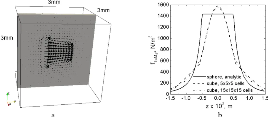
a b

Figure 5. Numerical results for a cubic particle 1mm×1mm×1mm inside the infinite media. a: Vector field of the thermoelectric magnetic force presented in a sub-domain in a plane (yz) which passes through the centre of the particle. b: TEMF distribution along the z-axis with the origin in centre of the particle, analytical solution for a sphere is given as a reference.

5.3. Comparison of the results of numerical simulation and experimental observation

Because of the size of the volume where solidification of Al-4wt%Cu was performed some effects related to the constraints of the thermoelectric current compared with the analytical problems could be expected. Properties of the solid and liquid phases were similar to that given in the table 1. Geometry

(9)

of the calculation domain for modelling with AEQUATIO was taken as the one presented in figure 1 but with the thickness of 300µm. A sub-domain containing a cubic particle 100µm×100µm×100µm was placed near the centre of the calculation domain. We considered sub-domains of two sizes: 200×400µm×400µm and 200×800µm×800µm with the same space discretization. One can observe that the size of the sub-domain affects results of calculation drastically both in terms of the smoothness of the solution and in values as shown in figure 6.

a b

Figure 6. Calculated distribution of the y-component (a) and z-component (b) of the TEMF within sub-domains along the z-axis which passes through the centre of each sub-domain, parallel to the thermal gradient. Solid line and dashed lines are for sub-domain 200×400µm×400µm and 200×800µm×800µm, respectively. A particle is between -0.05·10-3_{m and 0.05·10}-3_m.

The second sub-domain provides smooth variation of the y-component of the thermoelectric magnetic force in the liquid surrounding the particle (dashed line in figure 6a) and smaller values for its z-component (dashed line in figure 6b) which appear due to numerical errors. Furthermore, the maximal value calculated for the fTEMF,y in this case is about 1600N/m3, i.e. the same value as obtained for a cubic particle in the infinite media in previous section (figure 5b). The values of the force at the boundary of the particle at z=±0.05·10-3_{m are also similar to the values obtained in previous section. In} other words, the thermoelectric current is not affected by the presence of the walls of the domain.

For further calculation of the particle velocity and trajectory a larger sub-domain was used. Due to stable thermal gradient there is no thermo-convection. According to experimental observation, particle is moving preferentially in an horizontal direction with some oscillations in vertical direction. These oscillations may be attributed to solute convection. In the liquid phase, Lorentz force decrease sharply. It is expressed as a function of r3_{, with r the distance from the center of the particle. We suppose that}

the liquid flow around the particle will change its shape but will not affect the motion.

The components of the thermoelectric magnetic force integrated over the volume of the particle according to the (10) are FTEM=(0.0, 1.7037·10-9, 9.39·10-11). The z-component of the TEMF, as said above, appeared because of the numerical errors and was 18 times smaller than the y-component. According to (9) a viscosity drag force is required to calculate the evolution of the particle velocity. Navier-Stokes equations are not implemented yet into AEQUATIO toolbox and because of this an analytical approximation was used in calculations. For a sphere with the radius R, the coefficient in (11) is known to beA=6

πµ

_LR. As approximation, the equivalent radius for a cubic particle can be taken R_eq =D/

π

where D is the size of the cube side to keep the same cross section of the particle that in our case gives Req=56.4 µm. Since the particle moves in the horizontal direction the temperature distribution does not change around it and therefore thermoelectric magnetic force does not change either. The stationary situation when TEMF and viscous drag force are equal occurs less than in a half of the second as shown in eq.(12) and the value of the stationary velocity is given as

(10)

eq S TEM S TEM S _R F A F V πµ 6 , , ! ! ! = =

For our case this gives a velocity of 670µm/s. This value is about 3 times larger than the one estimated from the experimental results and theoretically in [9]. This difference can be explained by following factors. The first one is related to uncertainty in the physical properties of the materials, especially for the Seebeck coefficients. Thus in [9] other values for SS and SL were used and their difference was two times smaller than in the present work, i.e. the resulting TEMF was also two times smaller. The second reason is that the dendrite fragment does not have a regular shape: even if it has a spherical envelope its solid fraction is smaller that decreases the total TEMF and increases viscous drag force. For a cube integrated TEMF is approximately 2 times higher than the one of equivalent sphere. Finally, a drag force may be higher than we used in our approximation due to a small thickness of the crucible.

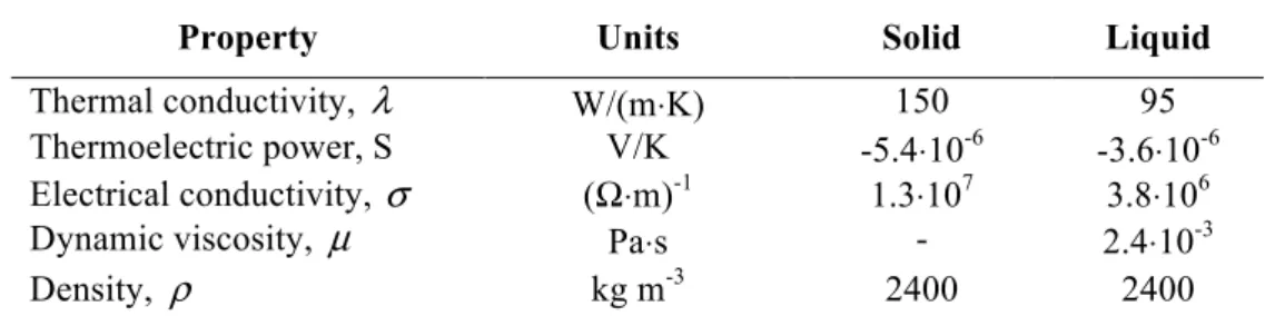
Table 1. Properties used in simulations.

Property Units Solid Liquid

Thermal conductivity, λ _W/(m⋅K) 150 95

Thermoelectric power, S V/K -5.4⋅10-6 _-3.6⋅10-6

Electrical conductivity, σ (Ω⋅m)-1 _1.3⋅107 _3.8⋅106

Dynamic viscosity, µ Pa⋅s - 2.4⋅10-3

Density, ρ kg m-3 ₂₄₀₀ ₂₄₀₀

6. Conclusion

Numerical simulations made with multi-physics multi-grid numerical toolbox AEQUATIO showed good agreements with analytical solutions. Oscillations of numerical solutions observed in the present work are probably related to a straightforward implementation of the phase function and can be suppressed via correct choice of the latter. In simulations of the experimental problem, constraints effect for the electric current related to the size of the simulation domain were not found. However, strong sensitivity of the results to the space discretization was revealed.

References

[1] Shercliff J A 1979 J. Fluid Mech. 91 231

[2] Karklin J and Mikelson A J 1981 J. Cryst. Growth 52 524

[3] Gelfgat Yu and Gorbunov L A 1989 Dokl. Acad. Nauk SSSR 306 667 [4] Li Xi 2007 Thèse de docteur de l’INP Grenoble

[5] Yasuda H., Kato S, Shinba T, Nagira T, Yoshiya M, Sugiyama A, Umetani K and Uesugi K 2010 Mat. Sci. Forum 649 131

[6] Nguyen-Thi H, Wang J, Salloum Abou Jaoude G, Reinhart G, Kaldre I, Mangelinck N, Ren ZM, Buligins L, Bojarevics A, Fautrelle Y, Budenkova O and Lafford T 2014 Mat. Sci. Forum 790-791 420

[7] Kao A and Pericleous K, 2012 IOP Conf. Ser.: Mater. Sci. Eng. 33 012045

[8] Li Xi, Gagnoud A, Wang J, Li Xialong, Fautrelle Y, Ren Z M, Lu X, Reinhart G and Nguyen-Thi H 2014 Acta Mater. 73 83

[9] Wang J, Fautrelle Y, Ren Z M, Li X, Nguyen-Thi H, Mangelinck-Noel N, Salloum Abou Jaoude G, Zhong Y B, Kaldre I, Bojarevics A and Buligins L, 2012 Appl. Phys.Lett. 101 251904 [10] Humbert E, Wang J, Budenkova O, Ren Z M and Fautrelle Y 2014 Proc. Int. Sci. Colloquium

Modelling for Electromagnetic Processing, MEP 2014, Hannover 43

[11] Du Terrail Couvat Y, Gagnoud A and Triwong P 2008 Proc. NUMELEC 2008, Belgique, [12] Kaldre I, Fautrelle Y, Etay J and Buligins L 2011 Mod. Phys. Lett. 25 731