HAL Id: hal-01662966
https://hal.archives-ouvertes.fr/hal-01662966
Submitted on 18 May 2018
HAL is a multi-disciplinary open access
archive for the deposit and dissemination of
sci-entific research documents, whether they are
pub-lished or not. The documents may come from
teaching and research institutions in France or
abroad, or from public or private research centers.
L’archive ouverte pluridisciplinaire HAL, est
destinée au dépôt et à la diffusion de documents
scientifiques de niveau recherche, publiés ou non,
émanant des établissements d’enseignement et de
recherche français ou étrangers, des laboratoires
publics ou privés.
nonintegrable Hamiltonian
Shun Ogawa
To cite this version:
Shun Ogawa.
Linear and nonlinear response of the Vlasov system with nonintegrable
Hamilto-nian. Physical Review E , American Physical Society (APS), 2017, 96 (1), pp.012112
�10.1103/Phys-RevE.96.012112�. �hal-01662966�
Linear and nonlinear response of Vlasov system with non-integrable Hamiltonian
Shun Ogawa1,∗
1Aix Marseille Univ., Université de Toulon, CNRS, CPT, Marseille, France
Linear and nonlinear response formulae taking into account all Casimir invariants are derived without use of angle-action variables of a single particle (mean-field) Hamiltonian. This article deals mainly with the Vlasov system in a spatially inhomogeneous quasi-stationary state whose associating single particle Hamil-tonian is not integrable and has only one integral of the motion, the HamilHamil-tonian itself. The basic strategy is to restrict the form of perturbation so that it keeps Casimir invariants within a linear order, and the single particle’s probabilistic density function is smooth with respect to the single particle’s Hamiltonian. The the-ory is applied for a spatially two dimensional system and is confirmed by numerical simulations. A nonlinear response formula is also derived in the similar manner.
I. INTRODUCTION
Long range interaction systems show several phenomena which are out of scope of the equilibrium statistical me-chanics [1, 2]. One of them is that such a system is of-ten trapped in out-of-equilibrium quasi-stationary states (QSSs) whose duration gets to be longer as the number N of elements in a system and diverges when the large pop-ulation limit N → ∞ is taken [1–5]. Then, if the system of interest is huge enough, the relaxation time is so long that one cannot see the thermal equilibrium state. It is hence in-teresting to investigate the non-equilibrium statistical me-chanics or thermodynamics of QSSs. In particular, the topic of this article is effect of external forces in the QSSs.
When N is huge enough, temporal evolution of the long-range interaction system is well described by the Vlasov equation [6–8] (also called the collisionless Boltzmann equation [3]) which describes evolution of a density func-tion defined on a µ-space, a single particle phase space. The QSSs are interpreted as stable stationary solutions to the Vlasov equation [4]. The Vlasov equation has unique so-lutions for each given initial state [7, 8], and thus the QSSs depend not only on macroscopic variables such as temper-ature and energy but also on mesoscopic things, details of the single particle density function. Thus the study on re-sponses to external forces in QSSs should be based on the Vlasov equation.
The linear response theory for the Vlasov systems has been developed for stability analysis in self-gravitating sys-tems [3], for looking into plasmas responses in magnetically confined plasmas [9], for computing time-asymptotic re-sponse to the external forces of long-range interaction sys-tems in both spatially homogeneous [10] and inhomoge-neous [11] QSSs and of a fluid systems [12]. By use of this theory, critical phenomena in QSSs [13] are investigated, and some informations of unforced systems are extracted by observing responses to oscillating external forces [11]. Further, the nonlinear response theory has been developed
∗[email protected], Author’s current address: RIKEN BSI, 2-1
Hiro-sawa, Wako, 351-0198 Japan
to investigate the response to the finite size external forces in QSSs near or on the critical point in which the linear re-sponse theory does not work [14, 15]. These rere-sponse for-mulae have been derived only when the single particle ef-fective Hamiltonian is integrable and the angle-action vari-ables are used for solving test particle dynamics.
Analyzing the linearized equation with the non-integrable effective Hamiltonian is practically important, because systems in multi-dimensional spaces are more realistic (for example, self-gravitating systems in the three dimensional (3D) space, magnetically confined hot plas-mas) and their effective Hamiltonians are non-integrable in general. To tackle this problem, one method to take into account constraints a posteriori is proposed to obtain linear response formulae approximately [16]. This method pro-vides canonical (taking into account the normalization) and micro-canonical (taking into account the normalization and the energy concervation) linear responses and other kinds of linear responses with a finite number of constraints systematically. However one cannot obtain isolated one with this method because it is practically impossible to take into account infinitely many Casimirs constraints with this method. The same problem lies in the stability analysis of the Vlasov equation [17]. If the effective Hamiltonian is not integrable, it was impossible to obtain the precise stability criterion with a finite time step procedure in general, since one should obtain an infinite number of Lagrangian multipliers associated with the Casimir’s constraints [18].
The above problems in the linearized equation should be solved as the first step to understand the dynamics around the QSSs with non-integrable effective Hamiltonian. Af-ter that, we will be able to continue tackling more difficult problems on nonlinear Landau damping, nonlinear stabil-ity, nonlinear response, critical phenomena and their uni-versality, and finite N effects.
In this article, we firstly obtain the linear response of the Vlasov system in the multi-dimensional space without solv-ing the linearized Vlasov equation and without ussolv-ing the angle-action variables. Let an initial state without external field be f0(q, p) and a final state fh(q, p) after exerting
ex-ternal field h. The linear response is obtained by restricting the form of accessible perturbation by assuming smooth-ness of fhwith respect to h, and by taking into account the
constraint conditions that the perturbation should be on a tangent “plane” of a constraint surface at f0.
Further, we shall mention the nonlinear response for-mula [14] derived via the transient (T-) linearization method developed by Lecellotti and Dorning [19–21] to analyse the plasmas oscillation and nonlinear Landau damping. In this theory, the Vlasov equation is linearized around an “unknown” asymptotic stationary state. Solving this equation, we obtain a self-consistent equation determin-ing the asymptotic state. The asymptotic solution is ob-tained by redistributing the initial density function along iso-asymptotic effective Hamiltonian sets, and this formula is called rearrangement formula [22]. The same formula is also derived for predicting the QSSs in a 1D system [23] and a 3D self-gravitating system [24] via the another consider-ation when non-stconsider-ationary initial states satisfy a (general-ized) viral condition and there is no parametric resonance. It is derived the rearrangement formula keeps Casimir in-variants at the order of T-linearization. Then, the nonlinear response formula is derived in a similar manner to derive the linear response formula in this article.
This article is organized as follows: The model and the dy-namics in a mean-field limit N → ∞ are firstly introduced in Sec. II, and the explicit form of constraint condition com-ing from Casimir invariants is derived in Sec. III. Based on this constraint condition, the linear response formula is de-rived in Sec. IV and several examples are exhibited in Sec. V. We derive the nonlinear response formula and make a brief comment on problems in the T-linearized Vlasov equation for spatially multi-dimensional systems in Sec. VI, and sum-marize this article in Sec. VII.
II. MODEL AND ITS DYNAMICS A. Model and Vlasov equation
Let us consider a system with long-range interaction whose Hamiltonian is HN= N ∑ i=1 ∥pi∥2 2 + 1 2N N ∑ i , j=1 V(qi− qj ) + h(t)∑N i=1Φ(qi ), (1)
where qi denotes configuration of the i -th particle, pi its conjugate momentum, V the inter-particles (-cites) poten-tial, and h(t )Φ(qi) interaction between the external field
h and the i -the particle. Taking the mean-field limit N →
∞ [6–8], the temporal evolution of this system can be
described in terms of the single-particle density function
f (q, p, t ) which is a solution to the Vlasov equation, ∂f
∂t +
{
H [f ], f}= 0, (2)
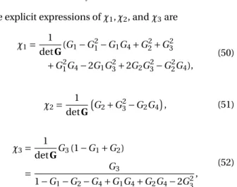
whereH [f ] is an effective single-particle Hamiltonian,
H [f ] =∥p∥2
2 + V [f ](q) + h(t)Φ(q), (3)
and {a, b} is the Poisson bracket given by {a, b}=∂a ∂p· ∂b ∂q− ∂a ∂q· ∂b ∂p. (4)
The system is initially in a QSS, f0, and the effective
Hamil-tonian
H0(q, p)= H [f0](q, p)=∥p∥ 2
2 + V [f0](q) (5)
has only one integral of motion, H0 itself. The f0 is
ex-pressed as f0(q, p)= F0
(
H0(q, p)
)
by use of a monotoni-cally decreasing function F0. This assumption is
reason-able when we are interested in the asymptotic behavior of perturbations around the formally stable solutions to the Vlasov equation [4, 5, 17, 25]. The formal stability is defined in terms of positive or negative definiteness of second varia-tion of an invariant funcvaria-tional around f0which is a solution
to the optimization problem:
maximizing S [f ] = Ï s( f )d qd p, subject to 1= N [f ] = Ï f d qd p, E= E [f ] = Ï ∥p∥2 2 f d qd p+ 1 2 Ï V [f ]f dqdp (6)
where s is a convex function. A formally stable solution is linearly stable [25]. By solving the optimization problem, we have a solution,
f0(q, p)= (s′)−1(βH0+ α) ≡ F0(H0), (7)
where s′ denotes d s(x)/d x, and α and β are Lagrangian multipliers with respect to the normalization and the en-ergy conservation. Since s is convex, then the inverse of its first derivative (s′)−1is a strictly decreasing function. The parameterβ must be positive.
B. Linear response
The external field h(t ) is turned on and it converges to a constant h(t )→ h as t → ∞. In the previous studies [10–12] the asymptotic linear responseδf is obtained by solving the linearized Vlasov equation around f0,
∂gp
∂t + {H0, gp}+ {V [gp]+ h(t))Φ, f0}= 0,
where gp(t )∼ O(h) is a perturbation around f0, and by
tak-ing the limit,δf = limt→∞gp(t ). The angle-action variables
of the HamiltonianH0is necessary to solve the linearized
Vlasov equation, but it is impossible in general for multi-dimensional systems. To avoid this problem, we focus on constraint conditions restricting a form of perturbations, and we obtain the linear responseδf without solving the linearized Vlasov equation.
III. CASIMIR INVARIANTS
We assume that f and its derivatives converge to 0 rapidly enough as∥p∥ → ∞. Further, f and its derivatives are as-sumed to vanish on the boundary of spatial domain or the system has periodic boundary condition with respect to q. Under these assumptions, it is shown (see Appendix. A) that the Vlasov equation keeps values of Casimir functionals,
C [f ] =
Ï
c(f (q, p, t ))d qd p, (8)
for any smooth function c. The linearized Casimir conser-vation condition is expressed as that the accessible pertur-bationδf satisfies
Ï
c′(f0(q, p)
)
δf (q,p)dqdp = 0, (9)
where c′(x) = dc/dx for any smooth function c. Since
f0(q, p)= F0
(
H0(q, p)
)
, F0 is a monotonically decreasing
function, and c is chosen arbitrarily, the constraint condi-tion (9) is equivalent to the condicondi-tion,
0= Ï R(H0(q, p) ) δf (q,p)dqdp = Ï R(H0(q, p) ) 〈δf 〉H0(q,p)d qd p, (10)
for any function R [17]. The second equality is shown as fol-lows: Ï R(H0(q, p) ) 〈δf 〉H0(q,p)d qd p= Ï R(H0(q, p) )Îδf (q′, p′)δ(H 0(q, p)− H0(q′, p′) ) d q′d p′ Î δ(H0(q, p)− H0(q′′, p′′) ) d q′′d p′′ d qd p = Ï R(H0(q, p) )[Ï δf (q′, p′)δ(H0(q, p)− H0(q′, p′)) S(H0(q, p) ) d q′d p′ ] d qd p = Ï δf (q′, p′) [Ï R(H 0(q, p) ) δ(H0(q, p)− H0(q′, p′) ) S(H0(q, p) ) d qd p ] d q′d p′ = Ï δf (q′, p′)R ( H0(q′, p′) ) S(H0(q′, p′) ) S(H0(q′, p′) ) d q′d p′= Ï R(H0(q, p) ) δf (q,p)dqdp, (11)
where S denotes a volume of iso-H0set,
S(E )=
Ï
δ(E− H0(q′, p′)
)
d q′d p′. (12)
More generally it is possible to show as in the 1D case [14] that Ï 〈a〉H0(q,p)b(q, p)d qd p= Ï a(q, p)〈b〉H0(q,p)d qd p, (13) for the functions a and b when〈a〉H0b and a〈b〉H0are
in-tegrable. Thus it has been shown that the condition (10) is equivalent to
〈δf 〉H0= 0, for almost every (q,p). (14)
IV. LINEAR RESPONSE FORMULA A. Implicit form of linear response
After that the external field is exerted and the limit t→ ∞ is taken, the effective Hamiltonian becomes
Hh(q, p)= H0(q, p)+ δV (q) + hΦ(q) +O(h2), (15)
where the linear responseδV ≡ V [δf ]. Let the initial and final states be respectively as:
f0(q, p)= F0 ( H0(q, p) ) =G0 ( H0(q, p) ) 〈G0〉µ , fh(q, p)= Fh ( Hh(q, p) ) =Gh ( Hh(q, p) ) 〈Gh〉µ , (16)
where〈a〉µ=Îad qd p and
Gh(Hh)= G0(Hh)+ hG1(Hh)+O(h2)
= G0(H0)+G′0(H0)(Hh− H0)+ hG1(H0)+O(h2).
(17)
Expanding fharound f0, we have
fh= f0+ G′0(H0)(δV + hΦ) +G1(H0) 〈G0(H0)〉µ − ⟨ G′0(H0)(δV + hΦ) +G1(H0) ⟩ µG0(H0) 〈G0(H0)〉2µ +O(h2). (18)
We then obtain the linear response, δf ≡ F0′(H0)(δV + hΦ) + G1(H0) 〈G0(H0)〉µ −⟨F0′(H0)(δV + hΦ) ⟩ µF0(H0)− 〈G1(H0)〉µF0(H0) 〈G0(H0)〉µ (19)
by taking the linear order. The function G1is determined so
that〈δf 〉H0= 0, that is,
G1 〈G0〉µ= 〈G1〉µ 〈G0〉µF0− F ′ 0(H0)〈δV + hΦ〉H0 + F0(H0) ⟨ F0′(H0) (δV + hΦ) ⟩ µ , (20)
where F0′(H0)= G′0(H0)/〈G0(H0)〉µ. The response is
there-fore implicitly given by
δf = F0′(H0) ( δV (q) −⟨δV (q)⟩H0) + hF0′(H0) ( Φ(q) −⟨Φ(q)⟩H0). (21)
Solving the implicit linear response formula (21) by using bi-orthogonal basis, we obtain explicitly the linear response taking into account the constraint conditions.
We make a comment on the case that there exist two integrals and f0 depends on the both of them. LetL =
Î
L(q, p) f d qd p be an additional integral (the angular
mo-mentum density for example). We consider the optimiza-tion problem (6) and we add the addioptimiza-tional constraintL = Const. to Eq. (6). A solution f0 depends onH0and L as
f0= F0
(
βH0+ νL
)
whereβ and ν are Lagrangian multipli-ers. Thus the accessible perturbation satisfies
〈δf (q,p)〉(βH0(q,p)+νL(q,p))= 0, (22)
where the bracket〈•〉(βH0(q,p)+νL(q,p))means the average
taken over iso-(βH0+νL) set. It should be noted that a form
of constrained perturbation depends on how f0depends on
H0and L. We should find ways to restrict the form of
per-turbations for each stationary state.
If H0 has three independent integrals of motion, we
can use angle-action variables and can solve the linearized Vlasov equation.
B. Explicit form of linear response
We introduce the bi-orthogonal basis [3, 26, 27], {di(q)}i∈I
and {ui(q)}i∈I′, where the setsI′ andI satisfy I′⊂ I ⊂ Z. A perturbation of spatial density is spanned by the base {di}i,
δρ(q) =
∫
δf (q,p)dp =∑
i∈I
ai(t )di(q). (23)
The base {ui}i is introduced as
ui(q)≡ (V ∗ di)(q)≡
∫
V (q− q′)di(q′)d q′, (24)
and the orthogonal relation ∫
di(q) ¯uj(q)d q= λjδi j (25)
holds, whereλi ̸= 0 when i ∈ I′and it vanishes otherwise,
andδi jis the Kronecker delta. The upper bar denotes
com-plex conjugate. Integrating the terms includingδf or δV in Eq. (21) with respect to p, we have
∫ δf dp − ∫ F0′(H0) ( δV (q) −⟨δV (q)⟩H0)d p =∑ i∈I ai [ di− ∫ F0′(H0) ( ui(q)− ⟨ ui(q) ⟩ H0 ) d p ] . (26)
Multiplying ¯uj to both sides and integrating them with
re-spect to q, we have, ∑ i∈I′ai [ λjδi j− ∫ F0′(H0) ( uiu¯j− 〈ui〉H0 ⟨ ¯ uj ⟩ H0 ) d pd q ] =∑ i∈I′ [ λjδj i− ∫ F0′(H0) ( ¯ ujui− ⟨ ¯ uj ⟩ H0〈ui〉H0 ) d pd q ] ai . (27) Let F= (Fj i)(i , j )∈I′×I′ be a matrix whose elements are given by Fj i= ∫ F0′(H0) ( ¯ ujui− ⟨ ¯ uj ⟩ H0〈ui〉H0 ) d pd q. (28)
We further assume that the term coupling with external force can be expanded as
Φ(q) =∑ i∈I′biui(q). (29) We then have h ∫ F0′(H0) ( Φ(q) −⟨Φ(q)⟩H0)d p = h∑ i∈I′ bi ∫ F0′(H0) ( ui(q)− ⟨ ui(q) ⟩ H0 ) d p, (30)
by integrating the term coming from external force in Eq. (21) with respect to p. Multiplying ¯uj to it and
integrat-ing with respect to q, we have, (as we have already done)
h∑
i∈I′
Fj ibi. (31)
Combining Eqs. (27) and (31), we get the linear equation de-termining {ai}i∈I′, ∑ j∈I′ ( λjδi j− Fi j ) aj= h ∑ j∈I′ Fi jbj. (32)
Introducing symbols x = (xi)i∈I′ for x = a,b and Λ = diag(λi)i∈I′, we can simplify the equation as follows:
(
and it is solved as
a= h(1 − F)−1Fb= hD−1(1− D)b, (34)
where 1 denotes the unit matrix and D = 1 − Λ−1F.
The maximal-eigenvalue of D is zero when f0 might be
marginally stable, and corresponds to the critical point. When we apply Eq. (34) to 1D systems, This explicit re-sponse formula formally coincides with what is derived in Ref. [11].
V. EXAMPLES: HAMILTONIAN MEAN-FIELD MODELS A. One dimensional case
Let us examine the proposed theory by use of the Hamil-tonian mean-field (HMF) model whose HamilHamil-tonian is
H= N ∑ i=1 p2i 2 − 1 2N ∑ i̸=j cos(qi− qj)− h N ∑ i=1 cos qi. (35)
where h is an external field, pi ∈ R, qi ∈ [−π,π) for i =
1, 2,··· ,N. In the equilibrium state, this model shows sec-ond order phase transition at the temperature T = 0.5, where the Boltzmann’s constant kB= 1. By use of the
lin-ear and nonlinlin-ear response formulae, the critical phenom-ena in the equilibrium state and QSSs for the isolated HMF model are investigated and it is shown that the Casimir constraints bring about the non-classical critical exponents [13–15]. We here check that the present method yields the linear response formula same with the previously obtained one for the 1D HMF model. The effective Hamiltonian is
H =p2
2 − Ï
cos(q− q′) f (q′, p′, t )d q′d p′− h cosq. (36)
Applying Eq. (21) for the HMF model, we can derive the lin-ear response formula
δf = (−δM − h)F0′(H0)
(
cos q− 〈cosq〉H0
)
, (37) where δM =Îcos qδf dqdp. Multiplying cosq to both sides and integrating over theµ-space, we obtain the linear response as δM =1− D D h, (38) where D= 1 + Ï F′(H0) ( cos2q− 〈cosq〉2H0 ) d qd p. (39)
This is equivalent to the linear response formula obtained in Ref. [13].
For more general 1D systems it is obvious that Eq. (21) is equivalent to the linear order of the nonlinear response formula derived in Ref. [15].
V(x,y)
x
y
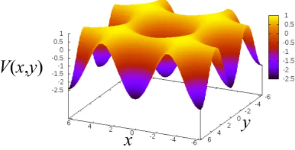
FIG. 1. (Color online) The effective potential of the Hamilto-nian (41). A minimum point is at (0, 0) and minV = −2M − P. Sad-dle points are at (±π,0) and (0,±π) and V = P. A maximum point
are on (±π,±π) and maxV = 2M − P, where M > P > 0.
B. Two dimensional case
We next examine our theory in the 2D system whose Hamiltonian is H=∑N i=1 ∥pi∥2 2 − hx N ∑ i=1 cos xi− hy N ∑ i=1 cos yi − 1 2N ∑ i̸=j [ cos(xi− xj)+ cos(yi− yj) +cos(xi− xj) cos(yi− yj) ] , (40)
where qi = (xi, yi)∈ [−π,π)2for i= 1,2,··· ,N [28, 29]. Let
us assume the initial QSS f0with hx = hy= 0 is even with
respect to both x and y. Then, the effective Hamiltonian is
H0=
p2x+ p2y
2 + V (x, y),
V (x, y) = −Mxcos x− Mycos y− Pcccos x cos y,
(41) where Mx= Ï cos xρ(q)dq, My= Ï cos yρ(q)dq, Pcc= Ï cos x cos yρ(q)dq, (42)
and whereρ(q) =Î f (q, p)d p. The effective potential is
shown in Fig. 1.
To compute the linear response of the macroscopic ob-servables Mx, My, and Pcc to the external field hx = hy=
h, it is necessary to compute 〈cosx〉H0, 〈cos y〉H0, and
〈cosx cos y〉H0. We here set Mx= My= M and Pcc= P.
For any smooth function g depending only on q,〈g〉E is
expressed as follows (see derivation for Appendix B.)
〈g〉E= ∫ R2d p ∫ [−π,π)2g (q)δ ( H (q,p) − E)d q = 2π ∫ [−π,π)2g (q)Θ ( E− V (x, y))d q. (43)
SinceH0is even with respect to both x and y, we have
〈sinx〉H0= 〈sin y〉H0= 〈sinx cos y〉H0
= 〈sinx sin y〉H0= 〈cosx sin y〉H0= 0.
(44) WhenH0> 2M − P = maxV (x, y), we have
〈cosx〉H0= 〈cos y〉H0= 〈cosx cos y〉H0= 0. (45)
Then we have to compute 〈cosx〉H0, 〈cos y〉H0, and
〈cosx cos y〉H0whenH0< 2M − P, and these are exhibited
in Appendix C. We next derive an explicit form of linear re-sponses, δMx= Ï cos xδf dqdp, δMy= Ï cos yδf dqdp, δPcc= Ï cos x cos yδf dqdp. (46)
The following notations are introduced for simplicity;
G1= − Ï F0′(H0) ( cos2x− 〈cosx〉2 H0 ) d qd p= − Ï F0′(H0) (
cos2y− 〈cos y〉2 H0 ) d qd p, G2= − Ï F0′(H0) (
cos x cos y− 〈cosx〉H0〈cos y〉H0
)
d qd p= −
Ï
F0′(H0)
(
cos x cos y− 〈cosx〉2H0 ) d qd p, G3= − Ï F0′(H0) (
cos2x cos y− 〈cosx cos y〉H0〈cosx〉H0
) d qd p = − Ï F0′(H0) (
cos x cos2y− 〈cosx cos y〉H0〈cos y〉H0
) d qd p, G4= − Ï F0′(H0) (
cos2x cos2y− 〈cosx cos y〉2H
0
)
d qd p.
(47)
By use of them and Eq. (21), we have 1−G−G21 1−G−G21 −G−G33 −G3 −G3 1−G4 δMδMxy δPcc = hhxxGG12+ h+ hyyGG21 (hx+ hy)G3 (48) We therefore obtain the explicit linear response formula as follows:
δMx= χ1hx+ χ2hy, δMy= χ2hx+ χ1hy,
δPcc= χ3(hx+ hy),
(49)
where explicit expressions ofχ1,χ2, andχ3are
χ1= 1 det G(G1−G 2 1−G1G4+G22+G23 +G2 1G4− 2G1G23+ 2G2G32−G22G4), (50) χ2= 1 det G ( G2+G23−G2G4 ) , (51) χ3= 1 det GG3(1−G1+G2) = G3 1−G1−G2−G4+G1G4+G2G4− 2G23 , (52)
respectively, where the determinant of G, the matrix in the left hand side of Eq. (48), is
det G= (1 −G1+G2)
×(1−G1−G2−G4+G1G4+G2G4− 2G23
) . (53)
A way to compute terms including〈cosx〉H0,〈cos y〉H0, and
〈cosx cos y〉H0is exhibited in Appendix D.
When F0(H0) is spatially homogeneous, that is, M= P =
0, we have G2= G3= 0 and G1and G4(1−G1< 1 −G4when
M= P = 0) do not vanish. Thus the susceptibilities are χ1=
G1
1−G1
, χ2= χ3= 0 (54)
in the disordered phase.
We numerically confirm the linear response formula. The initial state is the Maxwell-Boltzmann type:
fMB(q, p)=
exp(−H0/T )
〈exp(−H0/T )〉µ. (55)
This system shows the first order phase transition [28] and there is no (meta-)stable homogeneous state with T < 0.5. The initial values of order parameters for T = 0.3 and 0.4 are exhibited in Table I. The external field hx= hy= h is
ex-erted. Theoretically obtained susceptibilities are exhibited in Table I when the temperature T= 0.3 and 0.4, so that the
initial equilibria are spatially inhomogeneous. We integrate an equation of motion derived from the Hamiltonian (40) by using a fourth order symplectic integrator [30], and com-pute the order parameters of N body systems, given
respec-TABLE I. Initial equilibria and zero-field susceptibilities
T M P dδMx/y/d h|h=0 dδPcc/d h|h=0
0.3 0.90223 0.81556 0.034428 0.059089 0.4 0.84269 0.71910 0.071298 0.099709
tively by MxcN(t , h)= 1 N N ∑ i=1cos xi(t , h), MycN(t , h)= 1 N N ∑ i=1 cos yi(t , h), MxsN(t , h)= 1 N N ∑ i=1 sin xi(t , h), MysN(t , h)= 1 N N ∑ i=1 sin yi(t , h), (56) PccN(t , h)= 1 N N ∑ i=1 cos xi(t , h) cos yi(t , h), PcsN(t , h)= 1 N N ∑ i=1 cos xi(t , h) sin yi(t , h), PscN(t , h)= 1 N N ∑
i=1sin xi(t , h) cos yi(t , h),
PssN(t , h)= 1 N N ∑ i=1sin xi(t , h) sin yi(t , h), (57)
for null amplitude h= 0 and non-zero h. We compare the theoretically obtained linear responseδMx,δMy, andδPcc
with the numerically obtained responses given respectively by δMN x (h)= ¯MxN(h)− ¯MxN(0), δMN y(h)= ¯MyN(h)− ¯MNy(0), δPN x y(h)= ¯Px yN(h)− ¯Px yN(0), (58)
where MxN, MyN, and Px yN are given by
MxN= √ MN xc 2 + MN xs 2 , MyN= √ MNyc 2 + MN ys 2 , Px yN = √ PccN 2 + PN cs 2 + PN sc 2 + PN ss 2 , (59)
and where upper bars in Eq. (58) denote the time average ¯ MxcN(h)= 1 τ ∫ t0+τ t0 MxcN(t , h)d t . (60)
For the 2D HMF model there is error between ¯MxN(0) and
M which is a solution to the self-consistent equation. We
then focus on the difference ¯MxN(h)− ¯MxN(0) rather than ¯
MxN(h)− M. We set t0= 200, τ = 200, N = 4 × 10⁶, and the
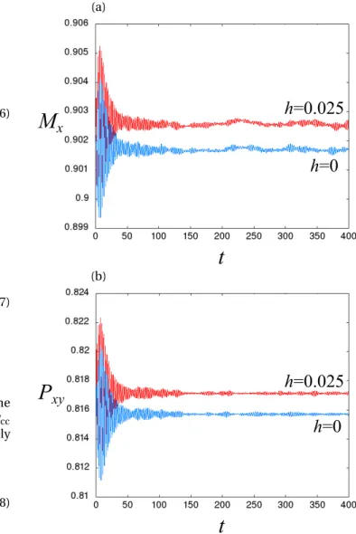
time stepδt = 0.05. Figure 2 shows that these t0andτ are
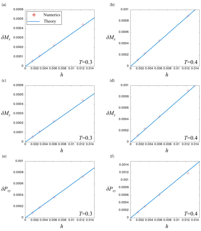
appropriate, and Fig. 3 shows that the numerically obtained results confirm the theory.
(a)
M
x
t
h=0.025
h=0
(b)t
h=0.025
h=0
P
xy
FIG. 2. (Color online) Time series of order parameters: The panel (a) is the time series for Mx and the panel (b) for Px y. The
tem-perature T= 0.3, the number of particles N = 4×10⁶, and the time
stepδt = 0.05. For each panel, the upper (red) curve is for h = 0.025 and the lower (blue) one for h= 0.
VI. NONLINEAR RESPONSE FORMULA
The nonlinear response formula [14] which is called the rearrangement formula in Ref. [22] keeps the Casimir invari-ants within an order of the T-linearization, the linearization around an asymptotic (A-) state fA(q, p)= limt→∞f (q, p, t )
assumed to be stationary. We derive the nonlinear response formula via the same strategy for deriving the linear re-sponse formula in the present article. We assume that the asymptotic effective Hamiltonian
HA= ∥p∥2/2+ VA+ hΦ, VA= V [fA], (61)
have only one integral of a single particle motion and fA
depends only onHA. Further fA= FA(HA) is assumed to
(a) (b)
h
T=0.3
M
xTheory
+
Numerics
h
T=0.4
M
x (c) (d)h
T=0.3
M
yh
T=0.4
M
y (e) (f )h
T=0.3
P
xyh
T=0.4
P
xyFIG. 3. (Color online)δMx,δMy, andδPx yas functions of h. The lines are the linear responses obtained theoretically and the crosses
are responses obtained numerically. We set temperature of the initial states as T= 0.3 (Left column, panels (a, c, e)) and T = 0.4 (Right column, panels (b, d, f )), and a number of particles N= 4 × 10⁶and the time stepδt = 0.05.
these assumptions, expanding Eq. (8) around fAas done in
Sec. III, the constraint condition coming from Casimir in-variants within an order of T-linearization can be expressed as Ï R(HA(q, p) )( f0(q, p)− fA(q, p) ) d qd p= 0, (62)
for any smooth function R onR. By use of Eq. (13), it is shown that Eq. (62) holds true if and only if
for almost every (q, p) in the µ-space. Deriving a self-consistent equation
VA(q)=
Ï
V (q− q′)〈f0〉HA(q′,p′)d q′d p′ (64)
from Eq. (63) and solving it, one can obtainHAand the
non-linear responseδf = fA− f0.
Is it possible to derive Eq. (63) for the multi-dimensional systems as done in Refs. [14, 15]? There is some difficulty to derive the same formula from the T-linearization method for the multi-dimensional systems. To see this, let us exhibit a sketch of this T-linearization method (see Refs. [14, 20–22] for details.) We firstly divide f (q, p, t ) in two ways: One is the naive perturbation decomposition,
f = f0+ gp, (65)
where gpis the perturbation around f0, and the other one is
the asymptotic-transient (AT) decomposition
f = fA+ gT, (66)
where gTis the T-term satisfying limt→∞gT= 0. According
to the AT decomposition, the potential is also decomposed as
V [f ] + h(t)Ψ = VA+ VT+ hΦ,
VT= V [gT]+ (h(t) − h)Φ.
(67) Substituting Eqs. (65) and (67) into the Vlasov equation, and omitting the nonlinear term coupling with the T-fieldVT, we
have the T-linearized Vlasov equation
∂f
∂t + {HA, f }+ {VT, f0}= 0. (68)
It should be noted that the nonlinearity still remains in the term {HA, f }. A solution fTLto the T-linearized equation is
implicitly given by fTL(q, p, t )= fON(q, p, t )+ fLA(q, p, t ), fON(q, p, t )= e−t{HA,•}f0(q, p), fLA(q, p, t )= − ∫ t 0 e−(t−s){HA,•} ( FT·∂f0 ∂p ) d s, (69)
where we introduce the operator {HA,•}a = {HA, a} for any
function a(q, p), and FT= −∂VT/∂q. The terms fONand fLA
are called O’Neil term and Landau term respectively [20, 21]. When the asymptotic stationary state fAexists, it can be
picked by taking the long-time average of fTL, and we have
fA(q, p)= limτ→∞ 1 τ ∫ τ 0 fTL(q, p, t )d t (70) within an order of the T-lineatization method. Then, our next job is to compute the long-time average of fON and
fLA, but there are several difficulties to this for the
multi-dimensional systems.
In the 1D systems, it is shown that lim τ→∞ 1 τ ∫ τ 0 e −t{HA,•}a(q, p)d t= 〈a〉 HA(q,p), (71)
by use of the angle-action variables ofHA[20, 21].
How-ever, in our case, the angle-action variables cannot be con-structed, so that it is unclear that this ergodic like formula holds true or not.
There is another problem, slowly algebraic damping of T-force-field FT. In Ref. [14] we use the fact that FT damps
rapidly (∼ t−νwithν ≥ 2) for the 1D systems [26] and lim
t→∞
∫ ∞
t FT(t )d t= 0
(72) when we compute limt→0fLA. Meanwhile, in the
multi-dimensional Vlasov systems [27] and the 2D Euler equations [31], the T-force-field FT damps as or slower than t−1, so
that the integral∫0∞FT(t )d t is not defined in the L1
mean-ing apparently. Sometimes, the transient part is asymptoti-cally FT≍ e−iΩtt−γ(0< γ ≤ 1) with Ω ̸= 0, and the integral
∫∞
0 FT(t )d t exists in the Riemannian meaning. In this case,
one should be more careful when one computes the inte-grals and takes the limit. It should be remarked that there exists a case thatΩ = 0 [27], so that it should be checked for each system.
The relation between the nonlinear response formula ob-tained by considering the constraint conditions and a solu-tion to the T-linearized Vlasov equasolu-tion might be an inter-esting future problem.
VII. SUMMARY AND PERSPECTIVE
The linear response formula has been derived without use of the analytic solution of the single particle orbit or the angle-action variables of the effective Hamiltonian. The present method improves the generalized linear response formula obtained in Ref. [16] when the back ground den-sity function is a monotonically decreasing function of the effective HamiltonianH0. The response formula (21)
re-sults in the one obtained in the previous studies for 1D sys-tems [10, 11, 13, 15], and is numerically confirmed by use of the 2D HMF model. Further the nonlinear response for-mula [14] has been derived via the same strategy, when the asymptotic solution fAto the T-linearized Vlasov equation is
monotonically decreasing function of the effective Hamilto-nianHA.
The nonlinear response theory based on the T-linearization method deals with the nonlinearity of order
O(hν) with 1 < ν < 2 [14]. It should be noted that it is difficult to obtain the nonlinear response of order higher than O(h2) successively via the proposed method, so that
the error O(h2) is unavoidable up to now. Let δfn be a
the nonlinear regime O(h2) is written as 0=Ï (R1(H0)δf2+ R2(H0)δf12 ) d qd p =Ï (R1(H0)〈δf2〉H0+ R2(H0)〈δf 2 1〉H0 ) d qd p, (73)
where R1= c′( f0) and R2= c′′( f0)/2. It is quite difficult to
obtain explicitlyδf2satisfying this equation for any c unlike
the linear regime. Then, the error O(h2) is unavoidable in both naive perturbation and T-liearization methods.
In the present article, the form of perturbation is re-stricted so as to subject to the constraint conditions com-ing from Casimir invariants at the linear order. By use of the form of constraint conditions (14), it is possible to take into account on the Casimir constraints when we derive the for-mal stability criterion without use of angle-action variables and this is a topic of forthcoming paper [32].
In this article, we exert the uniform external force to the systems without integrability. We may also consider the case that unperturbed system is integrable but an external force breaks its integrability. It might be an interesting fu-ture work, how the local chaos induced by the static exter-nal field affects meso- or macro-scopic properties of sys-tems. Such a phenomenon is found in a toy-model with one charged particle confined in cylindrical or toroidal mag-netic fields [33, 34].
ACKNOWLEDGMENTS
The author is grateful to Yoshiyuki Y. Yamaguchi and Xavier Leoncini for valuable discussions. He acknowledges the financial support of the A∗MIDEX project (n◦ ANR-11-IDEX-0001-02) funded by the “investissements d’Avenir” French Government program, managed by the French Na-tional Research Agency (ANR).
Appendix A: Conservation of the Casimir functionals (8)
It is shown that the Casimir functional (8) is conserved in the Vlasov dynamics. Taking the time derivative ofC [f ], we have dC [f ] d t = Ï ∂f ∂tc′( f )d qd p= − Ï {H [f ], f }c′( f )d qd p. (A1) Under the conditions asserted above Eq. (8), the boundary terms vanish and the left hand side of Eq. (A1) is
− Ï {H [f ], f }c′( f )d qd p= Ï H [f ]{f ,c′( f )}d qd p= 0 (A2) because { f , c′( f )}= 0. It is then shown that dC [f ]/dt = 0.
Appendix B: Derivation of Eq. (43)
We derive Eq. (43). The all we have to do is to perform integration with respect to p in the left hand side of Eq. (43);
∫ R2δ ( H (q,p) − E)d p= ∫ π −πdθp ∫∞ 0 pδ ( H (q,p) − E)d p = 2π ∫ ∞ 0 pδ ( p2 2 + V (x, y) − E ) d p= 2πΘ(E− V (x, y)), whereΘ(x) = 0 (resp.1) when x < 0 (resp. x ≥ 0) is the Heav-iside step function, and we have used the relation,
δ(f (x)) = ∑ x∗=f−1(0) δ(x − x∗) |f′(x∗)| , f′(x∗)̸= 0. Thus we have 〈g(q)〉E= ∫ (−π,π]2g (x, y)Θ ( E− V (x, y))d xd y ∫ (−π,π]2Θ ( E− V (x, y))d xd y . (B1)
Appendix C: Computation of〈cosx〉H0and〈cosx cos y〉H0
On the iso-H0curve, x and y satisfy
cos x= −H0+ M cos y M+ P cos y , cos y= − H0+ M cosx M+ P cosx . (C1) Thus ∫ (−π,π]2g (x, y)Θ ( H0− V (x, y) ) d xd y = 4 ∫ arccos(−H0+MM+P ) 0 d x
∫ arccos(−H0+M cosxM+P cosx ) 0
g (x, y)d y = 4
∫ arccos(−H0+MM+P )
0 d y
∫ arccos(−H0+M cos yM+P cos y )
0 g (x, y)d x (C2) forH0∈ [−2M − P,P] and ∫ (−π,π]2g (x, y)Θ ( H0− V (x, y) ) d xd y = 4 ∫ arccos(−H0−MM−P ) 0 d x ∫ π 0 g (x, y)d y + 4 ∫π arccos(−H0−MM−P )d x
∫ arccos(−H0+M cosxM+P cosx )
0 g (x, y)d y = 4 ∫ arccos(−H0−MM−P ) 0 d y ∫ π 0 g (x, y)d x + 4 ∫π arccos(−H0−MM−P )
∫arccos(−H0+M cos yM+P cos y ) 0
g (x, y)d x,
(C3)
forH0∈ [P,2M − P].
as follows respectively: When−2M − P < H0< P, we have
〈cosx〉H0= 〈cos y〉H0
= 8π σ(H0) ∫ arccos(−H0+MM+P ) 0 √ 1− (H 0+ M cosx M+ P cosx )2 d x, (C4)
〈cosx cos y〉H0=
8π σ(H0) ∫arccos(−H0+MM+P ) 0 cos x √ 1− ( H0+ M cosx M+ P cosx )2 d x, (C5) where σ(H0)= 8π ∫ arccos(−H0+MM+P ) 0 arccos ( −H0+ M cosx M+ P cosx ) d x, (C6) and where a range of the arccosine function is [0,π]. When
P< H0< 2M − P, we have
〈cosx〉H0= 〈cos y〉H0
= 8π σ(H0) ∫ π arccos(−H0−MM−P ) √ 1− (H 0+ M cosx M+ P cosx )2 d x, (C7)
〈cosx cos y〉H0=
8π σ(H0) ∫ π arccos(−H0−MM−P )cos x √ 1− ( H0+ M cosx M+ P cosx )2 d x, (C8) where σ(H0)= 8π ∫ π arccos(−H0−MM−P )arccos ( −H0+ M cosx M+ P cosx ) d x + 8π2arccos ( −H0− M M− P ) . (C9) Appendix D: Integral in Gn(n= 1,2,3,4)
The integralÎF0′(H0)〈cosx〉2H0d qd p included in G1and
G2is computed as follows; Ï F0′(H0)〈cosx〉2H0d qd p= 2π ∫ pd p ∫ F0′(H0)〈cosx〉2H0d q = 2π ∫ 2M−P −2M−PdH0F ′ 0(H0)〈cosx〉2H0 ∫ Θ(H0+ V (x, y) ) d q = 2π ∫ 2M−P −2M−PF ′ 0(H0)〈cosx〉2H0σ(H0)dH0, where p= ∥p∥ = √ 2(H0+ V (x, y) ) andσ(H0) is defined in
Eqs. (C6) and (C9). The similar terms in G2and G4are
com-puted in the same manner.
[1] A. Campa, T. Dauxois, D. Fanelli, and S. Ruffo, Physics of
Long-Range Interacting Systems, (Oxford University Press, Oxford,
2014).
[2] A. Campa, T. Dauxois, and S. Ruffo, Statistical mechanics and dynamics of solvable models with long-range interactions, Phys. Rep. 480, 57 (2009).
[3] J. Binney and S. Tremaine, Galactic dynamics, 2nd ed. (Prince-ton University Press, Prince(Prince-ton, NJ, 2008).
[4] Y. Y. Yamaguchi, J. Barré, F. Bouchet, T. Dauxois, and S. Ruffo, Stability criteria of the Vlasov equation and quasi-stationary states of the HMF model, Physica A 337, 36 (2004).
[5] J. Barré, F. Bouchet, T. Dauxois, S. Ruffo, and Y. Y. Yamaguchi, The Vlasov equation and the Hamiltonian mean-field model, Physica A 365, 177 (2006).
[6] W. Braun and K. Hepp, The Vlasov dynamics and its fluctua-tions in the 1/N limit of interacting classical particles, Com-mun. Math. Phys. 56, 101 (1977).
[7] R. L. Dobrushin, Vlasov equations, Funct. Anal. Appl. 13, 115 (1979).
[8] H. Spohn, Large scale dynamics of interacting particles, (Springer-Verlag, Heidelberg, 1991).
[9] A. Boozer, Physics of magnetically confined plasmas, Rev. Mod. Phys. 76, 1071 (2005).
[10] A. Patelli, S. Gupta, C. Nardini, and S. Ruffo, Linear response theory for long-range interacting systems in quasistationary states, Phys. Rev. E 85, 021133 (2012).
[11] S. Ogawa and Y. Y. Yamaguchi, Linear response theory in the Vlasov equation for homogeneous and for inhomogeneous quasistationary states, Phys. Rev. E 85, 061115 (2012). [12] P. H. Chavanis, Linear response theory for hydrodynamic and
kinetic equations with long-range interactions, Eur. Phys. J. Plus 128, 38 (2013).
[13] S. Ogawa, A. Patelli, and Y. Y. Yamaguchi, Non-mean-field crit-ical exponent in a mean field model: Dynamics versus statis-tical mechanics, Phys. Rev. E 89, 032131 (2014).
[14] S. Ogawa and Y. Y. Yamaguchi, Nonlinear response for external
field and perturbation in the Vlasov system, Phys. Rev. E 89,
052114 (2014).
[15] S. Ogawa and Y. Y. Yamaguchi, Landau-like theory for
univer-sality of critical exponents in quasistationary states of isolated mean-field systems Phys. Rev. E 91, 062108 (2015).
[16] A. Patelli and S. Ruffo, General linear response formula for non integrable systems obeying the Vlasov equation, Eur. Phys. J. D 68, 329 (2014).
[17] S. Ogawa, Spectral and formal stability criteria of spatially in-homogeneous stationary solutions to the Vlasov equation for the Hamiltonian mean-field model, Phys. Rev. E 87, 062107 (2013).
[18] A. Campa and P. H. Chavanis, A dynamical stability criterion for inhomogeneous quasi-stationary states in long-range sys-tems J. Stat. Mech, P06001 (2010).
[19] C. Lancellotti and J. J. Dorning, Critical Initial States in Colli-sionless Plasmas, Phys. Rev. Lett. 81, 5137 (1998).
[20] C. Lancellotti and J. J. Dorning, Time-asymptotic wave prop-agation in collisionless plasmas, Phys. Rev. E 68, 026406 (2003).
[21] C. Lancellotti and J. J. Dorning, Nonlinear Landau damping, Transp. Theory Stat. Phys. 38, 1 (2009).
[22] Y. Y. Yamaguchi and S. Ogawa, Conditions for predicting qua-sistationary states by rearrangement formula, Phys. Rev. E 92, 042131 (2015).
[23] A. C. Ribeiro-Teixeira, F. P. C. Benetti, R. Pakter, and Y. Levin, Ergodicity breaking and quasistationary states in systems with long-range interactions. Phys. Rev. E 89, 022130 (2014). [24] F. P. C. Benetti, A. C. Ribeiro-Teixeira, R. Pakter, and Y. Levin,
Nonequilibrium Stationary States of 3D Self-Gravitating Sys-tems, Phys. Rev. Lett. 113, 100602 (2014).
[25] D. D. Holm, J. E. Marsden, T. Ratiu, and A. Weinstein, Nonlin-ear stability of fluid and plasma equilibria, Phys. Rep. 123, 1 (1985).
[26] J. Barré, A. Olivetti, and Y. Y. Yamaguchi, Algebraic damping in the one-dimensional Vlasov equation, J. Phys. A: Math. Theor.
44 405502 (2011).
[27] J. Barré and Y. Y. Yamaguchi, On algebraic damping close to inhomogeneous Vlasov equilibria in multi-dimensional
spaces, J. Phys. A: Math. Theor. 46, 225501 (2013).
[28] M. Antoni and A. Torcini, Anomalous diffusion as a signature of a collapsing phase in two-dimensional self-gravitating sys-tems, Phys. Rev. E 57, R6233 (1998).
[29] A. Torcini and M. Antoni, Equilibrium and dynamical proper-ties of two-dimensional N -body systems with long-range at-tractive interactions, Phys. Rev. E 59, 2746 (1999).
[30] H. Yoshida, Recent progress in the theory and application of symplectic integrators, Celest. Mech. Dynam. Astron. 56, 27 (1993).
[31] F. Bouchet and H. Morita, Large time behavior and asymp-totic stability of the 2D Euler and linearized Euler equations, Physica D 239, 948 (2010).
[32] S. Ogawa, Stability criterion of spatially inhomogeneous solu-tions to Vlasov equation, submitted.
[33] B. Cambon, X. Leoncini, M. Vittot, R. Dumont, and X. Garbet, Chaotic motion of charged particles in toroidal magnetic con-figurations, Chaos: An Interdisciplinary Journal of Nonlinear Science 24, 033101 (2014).
[34] S. Ogawa, B. Cambon, X. Leoncini, M. Vittot, D. del Castillo-Negrete, G. Dif- Pradalier, and X. Garbet, Full particle orbit ef-fects in regular and stochastic magnetic fields, Phys. Plasmas