HAL Id: tel-01113135
https://hal.archives-ouvertes.fr/tel-01113135
Submitted on 4 Feb 2015
HAL is a multi-disciplinary open access archive for the deposit and dissemination of sci-entific research documents, whether they are pub-lished or not. The documents may come from teaching and research institutions in France or abroad, or from public or private research centers.
L’archive ouverte pluridisciplinaire HAL, est destinée au dépôt et à la diffusion de documents scientifiques de niveau recherche, publiés ou non, émanant des établissements d’enseignement et de recherche français ou étrangers, des laboratoires publics ou privés.
Assessment by an Exergy Analysis of High-fidelity
CFD-RANS Flow Solutions
A. Arntz
To cite this version:
A. Arntz. Civil Aircraft Aero-thermo-propulsive Performance Assessment by an Exergy Analysis of High-fidelity CFD-RANS Flow Solutions. Fluids mechanics [physics.class-ph]. Université de Lille 1, 2014. English. �tel-01113135�
Assessment by an Exergy Analysis of
High-fidelity CFD-RANS Flow Solutions
Submitted by
Aurélien Arntz
To obtain
Doctorate from Lille 1 University – Sciences and Technologies
Specialty
Mechanics and Energetics
Dissertation defended November 28th, 2014 to the Doctoral Committee composed of:
Mr. Olivier Atinault Research Engineer ONERA Supervisor
Pr. Allan Bonnet Professor ISAE Chairman
Pr. Philippe Devinant Professor Université d’Orléans Reviewer
Pr. Mark Drela Professor Massachusetts Institute of Technology Reviewer Pr. Alain Merlen Professor Université de Lille & ONERA Director
Dr. Simon Trapier Engineer Airbus Examiner
Dr. Zdenek Johan Design Engineer Dassault Aviation Invited
aéro-thermo-propulsives des avions civils par une
analyse exergétique de solutions haute-fidélité
CFD-RANS
Soutenue par
Aurélien Arntz
Pour l’obtention
Doctorat de Université de Lille – Sciences and Technologies
Spécialité
Mécanique et Energétique
Thèse soutenue le 28 Novembre 2014, devant le jury composé de :
M. Olivier Atinault Ingénieur de Recherche ONERA Examinateur
M. Allan Bonnet Professeur ISAE Président
M. Philippe Devinant Professeur Université d’Orléans Rapporteur
M. Mark Drela Professeur Massachusetts Institute of Technology Rapporteur
M. Alain Merlen Professeur Université de Lille & ONERA Directeur
M. Simon Trapier Ingénieur Airbus Examinateur
M. Zdenek Johan Ingénieur de Conception Dassault Aviation Invité
A great deal of effort has been deployed to make this document as easily readable as possible but I first would like to thank any native English-reader that would most certainly face some challenges in its reading. I would like to thank all the members of the Thesis Committee for having accepted to assess my work. A special thanks goes to Profs. M. Drela (MIT) and P. Devinant (Université d’Orléans) for doing me the honor of reviewing my thesis. The pioneering work of Prof. Drela has been very inspirational to my re-search and it is a privilege to have you evaluate this contribution. Ce manuscrit a également bénéficié des corrections/suggestions du président du jury, A. Bonnet (ISAE).
La direction de cette thèse a été assurée par A. Merlen qui a toujours su mettre le doigt sur les points qui n’étaient pas toujours pleinement acquis. Cela m’a permis d’approfondir des notions qui m’étaient inconnues. Le sujet de cette recherche a été proposé par O. Atinault qui en a assuré l’encadrement au quotidien. Merci Olivier pour ton enthousiasme jamais démenti et pour tes encouragements tout au long de ces trois années. Je tiens également à remercier D. Destarac pour sa constante disponibilité et réactivité, et pour m’avoir aidé à coder dans ffd72, ce qui m’a permis de me concentrer sur l’interprétation physique de l’analyse plutôt que sur des aspects purement numériques.
Le développement de la formulation théorique a largement bénéficié des préciseuses suggestions et cor-rections de D. Bailly. Merci Didier de m’avoir donné une idée des khôlles auxquelles j’ai échappé en prépa intégrée !
Cette thèse a été réalisée à l’Onera, dans l’unité avions civils du département d’aérodynamique ap-pliquée. Tout d’abord, merci à P. Champigny et J. Reneaux de m’avoir fait confiance pour mener à bien cette recherche. Cet environnement m’a amené à côtoyer de nombreuses personnes qui ont rendu ces trois années enrichissantes, tant sur le plan professionel que personnel: Michaël, Christelle, Fabien, David, Ludo, Antoine, Frédéric, Saloua, Vincent, Jean-Luc ... Merci pour les petits pains du vendredi !
La notion d’exergie m’était inconnue au début de cette thèse et m’a été introduite au travers d’une discussion avec S. Mouton. Merci Sylvain pour cette initiation qui m’a permis de découvrir une approche nouvelle pour la détermination des performances avions. Mes remerciements sont également adressés à S. Burguburu qui m’a beaucoup appris sur les moteurs d’avions ainsi qu’à N. Renard et S. Deck pour m’avoir aidé à appréhender les phénomènes liés à la turbulence.
J’aimerais également remercier C. Allafort du service Documentation de l’Onera qui m’a aidé à trouver plus de 60 documents (ouvrages et publications) avec un souci d’efficacité très apprécié.
Mes compagnons de route thésards ont également permis d’échanger sur cette expérience dans un cadre plus convivial. Merci à Loic, Mickaël, Romain, Amaury, Hélène, Mehdi, Anthony, Andrea ... Une dédicace spéciale est adressée au sas de décompression du bureau AY-02-36.
Il est parfois bon de se changer les idées, et pour celà la bande des mil’k’syn a été particulièrement ef-ficace, avec, dans le désordre, Yo, Dekap’s, Jpsi, Clairette, Firgui, Séba, Marion, Neiz, Le P’tiot, Gui, jOn, Rem’s, Colette, et surtout Michel (j’en oublie certainement). Merci à tous ceux qui ont fait le déplacement des quatre coins de la France pour venir voir la présentation de mes travaux qui a marqué le début d’une certaine liberté retrouvée !
J’ai également une pensée pour ma famille, spécialement pour mes parents et mon frère qui m’ont soutenu dans mon choix de me lancer dans la recherche. Enfin, merci à Aurélie pour tes encouragements tout au long de ces trois années et tout simplement merci de partager ma vie dans les moments difficiles.
According to BOREL, despite great efforts deployed by many scientists around the world, the exergy anal-ysis has not been completely standardized yet, neither in the terminology nor in the notation [31]. As a consequence, the author has been unable to find a commonly accepted nomenclature regarding the exergy analysis [38, 45, 149, 167, 168]. The one adopted here provides pedagogical advantages in agreement with the terminology proposed by RANT[129].
Formulation ˙
Aq = rate of heat anergy supplied by conduction (J.s−1) ˙
A∇T = rate of anergy generation by thermal mixing (J.s−1) ˙
Aφ = rate of anergy generation by viscous dissipation (J.s−1) ˙
Atot = rate of total anergy generation (J.s−1), = ˙Aφ+A˙∇T +A˙w ˙
Aw = rate of anergy generation by shock waves (J.s−1) ˙
A∗ = sum of exergy outflows and anergy generation (J.s−1), = ˙Em+ ˙Eth+A˙tot
D = aerodynamic drag (N)
˙
Eu = streamwise kinetic energy deposition rate (J.s−1)
˙
Ep = boundary pressure-work rate (J.s−1)
˙
Eφ = rate of thermal energy generation by viscous dissipation (J.s−1)
˙
Eq = rate of heat energy supplied by conduction (J.s−1)
˙
Eth = rate of thermal energy outflow (J.s−1)
˙
Eth(ρ) = outflow rate of thermal exergy associated with volume change ˙
Eth(T ) = outflow rate of thermal exergy at constant volume ˙
Ev = transverse kinetic energy deposition rate (J.s−1)
˙
EW = surroundings-work rate (J.s−1) ˙
Em = rate of mechanical exergy outflow (J.s−1), = ˙Eu+ ˙Ev+ ˙Ep ˙
Eprop = rate of exergy supplied by the propulsion system (J.s−1) ˙
Eprop,m = rate of mechanical exergy supplied by the propulsion system (J.s−1) ˙
Eprop,th = rate of thermal exergy supplied by the propulsion system (J.s−1) ˙
Eφ = rate of thermal exergy generation by viscous dissipation (J.s−1) ˙
Eq = rate of heat exergy supplied by conduction (J.s−1) ˙
Eth = rate of thermal exergy outflow (J.s−1)
FA = momentum change across the aircraft surface (N)
Fprop = momentum change across the propulsive surface (N)
FO = momentum change across the outer boundary (N)
Fx = streamwise resultant force acting on the vehicle (N)
γ = aircraft climb angle (deg)
Γ = weight specific aircraft energy height (m) n = unit normal vector
˜
n = unit normal vector for the shock wave ˆ
n = unit normal vector, = −n
ψi = engine intrinsic exergy efficiency
ψm = mechanical exergy efficiency
ψp = propulsive efficiency
qeff = effective heat flux by conduction (J.s−1), −keff∇T W = aircraft weight (N)
SA = aircraft surface SB = body surface
SO = outer boundary of the control volume SP = surface delimiting the propulsion system dTP = streamwise distance of the transverse plane
Fluid and Flow Properties
α = flow incidence relative to body (deg)
cp = mass specific heat capacity at constant pressure (J.kg−1.K−1)
cv = mass specific heat capacity at constant volume (J.kg−1.K−1)
e = mass specific internal energy (J.kg−1), = cvT
ε = mass specific flow exergy (J.kg−1), = δhi−T∞δs
h = mass specific enthalpy (J.kg−1), = e + p/ρ = cpT
hi = mass specific total/stagnation enthalpy (J.kg−1), = h + V2/2 keff = effective thermal conductivity (W.m−1.K−1), = cp(µ/P r + µt/P rt)
M = Mach-number
M⊥ = normal shock Mach-number
µ = laminar dynamic viscosity (kg.m.s−1) µt = turbulent dynamic viscosity (kg.m.s−1)
µeff = effective dynamic viscosity (kg.m.s−1), = µ + µt
p = static pressure (kg.m.s−2) pi = total/stagnation pressure (kg.m.s−2), = p [1 + (γ − 1)M2/2]) γ γ−1 P r = Prandtl-number P rt = turbulent Prandtl-number ρ = density (kg.m−3) Re = Reynolds-number
s = mass specific entropy (J.K−1.kg−1) ¯ ¯ S = strain rate (s−1) T = static temperature (K) Ti = total/stagnation temperature (K), = T [1 + (γ − 1)M2/2] Tw = wall temperature (K) ¯ ¯
τeff = effective viscous stress tensor (N), = (µ + µt)S¯¯ V = fluid velocity vector (m.s−1), = (V∞+u)x, vy, wz
Subscripts
adiab = adiabatic
∞ = quantity at freestream conditions TP = transverse plane
= quantity neglected numerically ( )c = quantity with numerical correction
Operators
∶= = equal by definition ≡ = numerically equivalent
J K = discontinuous jump of a quantity ˙
( ) = time derivative of a quantity, = d( )/dt δ( ) = quantity relative to freestream, = ( ) − ( )∞
∇( ) = gradients of a vector quantity, = [∂( )/∂x, ∂( )/∂y, ∂( )/∂z]T ∇ ⋅ ( ) = divergence of a vector quantity, = ∂( )/∂x + ∂( )/∂y + ∂( )/∂z
⊗ = tensor product
Acronyms
BLI = boundary-layer ingestion BW B = blended wing-body
ERC = exergy-recovery coefficient ESC = exergy-saving coefficient
ESF C = exergy specific fuel consumption EW C = exergy-waste coefficient
F P R = fan pressure ratio
M AC = mean aerodynamic chord
M F R% = non-dimensionalized massflow rate
Other Notations
∆hf = mass specific fuel heating value (J.kg−1)
dc = drag counts (10−4) ¯
¯
I = identity matrix λw = shock wave criterion
˙
mf = fuel mass flow (kg.s−1)
RICHARDP. FEYNMAN(1918–1988) Theoretical Physicist, Nobel Prize (1965)
Nomenclature . . . iii
Introduction . . . 1
OBJECTIVES ANDREQUIREMENTS . . . 4
1 Literature Review and Introduction to the Concept of Exergy 7 1.1 The Power Balance Method of DRELA. . . 8
1.1.1 Context . . . 8
1.1.2 Mechanical Energy Balance . . . 8
1.1.3 Experimental and Numerical Applications . . . 13
1.1.4 Advantages and Limitations . . . 14
1.2 Introduction to the Concept of Exergy . . . 14
1.2.1 Basics of Thermodynamics . . . 14
1.2.2 Literature Review on Exergy . . . 17
1.2.3 Exergy Analysis in Engineering . . . 19
1.3 Exergy Analysis in Aerospace Engineering . . . 19
1.3.1 System-level Flight Vehicle Design . . . 20
1.3.2 Propulsion Systems . . . 21
1.3.3 Energy Systems . . . 22
1.3.4 External Aerodynamics . . . 23
1.3.5 Entropy Generation from CFD-RANS . . . 24
1.4 Summary of the Key Findings . . . 25
2 Exergy-based Formulation for Aero-thermo-propulsive Performance 27 2.1 Exergy Balance for Aero-thermo-propulsive Performance Assessment . . . 28
2.1.1 Preliminary Considerations . . . 28
2.1.2 Exergy and the Combined First and Second Laws of Thermodynamics . . . 30
2.1.3 Physically-approximated Exergy Balance for Transonic Flows . . . 35
2.2 Further Specifications of the Formulation . . . 38
2.2.1 Near-field Propulsion Analysis . . . 39
2.2.2 Mid-field Outflows Characterization and Recovery . . . 41
2.2.3 Precisions on Dissipative Mechanisms . . . 44
2.2.4 Far-field Asymptotic Considerations . . . 46
2.3 Restriction to Aerodynamic Performance of Unpowered Airframe Configurations . . . 48
2.3.1 Restricted Exergy Balance for Aerodynamic Performance Assessment . . . 48
2.3.2 Connection to Momentum-based Far-field Drag Approaches . . . 49
2.4 Discussion on the Formulation . . . 50
2.4.1 Aerospace Vehicle Design Considerations . . . 51
2.5 Numerical Implementation of the Formulation . . . 54
2.5.1 Numerical Adaptation of the Theoretical Formulation . . . 54
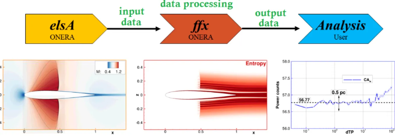
2.5.2 Post-processing Code Description . . . 57
2.6 Chapter Summary . . . 62
3 Validation of the Numerical Implementation for Unpowered Configurations 63 3.1 Methodology for Validation . . . 64
3.1.1 Methodology and Introduction to Test Cases . . . 64
3.1.2 Numerical Verification and Validation . . . 65
3.2 Validation for Viscous Phenomena in 2D Subsonic Flows . . . 67
3.2.1 Test Case Presentation . . . 67
3.2.2 Profile and Wake Analyses at M∞=0.30 . . . 68
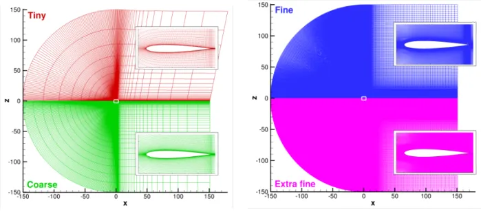
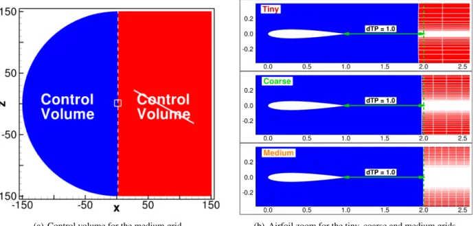
3.2.3 Grid Convergence Study on Drag Prediction . . . 71
3.2.4 Reynolds-number Sensitivity Analysis . . . 76
3.2.5 Summary of the Key Findings . . . 77
3.3 Validation for Viscous and Shock Wave Phenomena in 2D Transonic Flows . . . 79
3.3.1 Mach-number Sensitivity Analysis . . . 79
3.3.2 Profile and Wake Analyses at M∞=0.80 . . . 81
3.3.3 Grid Convergence Study on Drag Prediction . . . 83
3.3.4 Summary of the Key Findings . . . 90
3.4 Validation for 3D Transonic Flows . . . 91
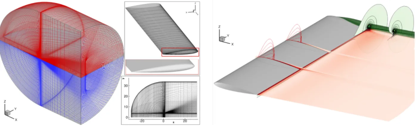
3.4.1 Test Case Presentation . . . 91
3.4.2 Wing and Wake Analysis in Terms of Anergy Generation . . . 94
3.4.3 Turbulence Model Sensitivity Analysis for Drag Prediction . . . 96
3.4.4 Summary of the Key Findings . . . 100
3.5 Validation for a Wing-Body Aircraft in Cruise Conditions . . . 101
3.5.1 Test Case Presentation . . . 101
3.5.2 Flow Field Analysis . . . 104
3.5.3 Grid Convergence Study on Drag Prediction . . . 108
3.5.4 Summary of the Key Findings . . . 117
3.6 Chapter Summary . . . 118
4 Aero-thermo-propulsive Performance Assessment of Powered Configurations 119 4.1 Methodology and Test Cases Introduction . . . 120
4.2 Verification of the Formulation for an Isolated Turbojet Engine . . . 122
4.2.1 Test Case Presentation . . . 122
4.2.2 Thermopropulsive Performance Assessment . . . 125
4.2.3 Near-field and Far-field Analyses . . . 128
4.2.4 Summary of the Key Findings . . . 131
4.3 Wake-ingesting Academic Configuration . . . 133
4.3.1 Test Case Presentation . . . 133
4.3.2 Aeropropulsive Performance Assessment . . . 136
4.3.3 Summary of the Key Findings . . . 142
4.4 Blended Wing-Body Architecture with Boundary Layer Ingestion . . . 143
4.4.1 Test Case Presentation . . . 143
4.4.2 Aeropropulsive Performance Assessment . . . 148
4.4.4 Summary of the Key Findings . . . 159
4.5 Heat Exchanger Integration on Aircraft . . . 160
4.5.1 Test Case Presentation . . . 160
4.5.2 Aerothermodynamic Performance Assessment . . . 163
4.5.3 Summary of the Key Findings . . . 168
4.6 Chapter Summary . . . 169
5 Summary, Conclusions and Perspectives 171 Summary . . . 171
Conclusions . . . 172
Perspectives . . . 173
A Theoretical Appendices 177 A.1 Drag/thrust Bookkeeping Methodology . . . 178
A.1.1 A Few Examples of Drag Performance . . . 178
A.1.2 Requirements for Drag/Thrust Bookeeping . . . 178
A.1.3 Thrust Definitions . . . 179
A.2 Aircraft Force Balance . . . 180
A.3 Vortex Drag Power for Inviscid Flows . . . 180
A.4 Exergy-based Range Equation . . . 181
A.5 Gibbs Equation in Terms of Stagnation Quantities . . . 182
A.6 Nearby-Strong Shock Losses . . . 183
A.7 Alternative Expression for the Effective Viscous Dissipation . . . 184
A.8 OSWATITSCH’s Development without Small Perturbations Assumption . . . 185
B Numerical Appendices 187 B.1 Entropy Flow Field over a NACA 0012 . . . 188
B.2 Validation for the Lift-induced Vortices in 3D Subsonic Flows . . . 189
B.2.1 Theoretical and Numerical Considerations . . . 189
B.2.2 Grid Convergence Study . . . 190
B.2.3 Summary of the Key Findings . . . 194
B.3 Wake-ingesting Configuration Grids . . . 195
List of Figures 197
List of Tables 203
Context
Market Forecast. A century after the first commercial flight made in January 1914, the air transportation industry has seen fantastic growth. Global Civil Market development is driven by many factors as diverse as market liberalization, infrastructure, network development, high speed rail, economic growth, environment, fuel price and emerging markets. The world air travel has grown by 5% per annum1since 1980 despite four recessions, two financial crises, two Gulf wars, two oil shock and more recently 9/11 which has resulted in many changes in the way people fly since then. Driven by emerging economies of Asia Pacific and Latin America, the same trend is expected for the next 20-year period. In fact, despite a different approach on how would the world travel demand evolve, last year, Airbus and Boeing agree that more than new 29,000 aircraft2will be necessary to meet this increasing demand over the 2013–2032 period [89, 160].
Environmental Concern. Today, around 2% of the CO2man-made emissions are attributed to air travel,
but this percentage may grow significantly in the future. Such growth has raised environmental concern and driven international institutions and major research agencies to set ambitious objectives of performance. Among these objectives emerged a dramatic reduction in both fuel combustion and noise/pollutant emis-sions: N Oxby 80% and CO2by 50% for the European Commission through ACARE [5].
In 2010, ONERA published an overview [86] of key technologies that require to be investigated based on four different scenarios identified a few years earlier in the Consave 2050 project [27]. Regarding air-craft, the current conventional tube and wing configuration has been justified by a function-driven approach: carrying people in the pressurized fuselage, lifting the airplane with wings and a propulsive system. Each separate part has been designed and optimized separately, their final assembly somehow providing an opti-mum. Because harder and harder improvements of the current architecture could only provide a short term answer to the future challenges, a breakthrough similar to the advent of the wide-bodies in the early 70’s is likely to be needed.
1
Keeping in mind that a 5% per year growth is equivalent to doubling the number of passengers every 15 years. 2
Airbus evaluates the potential to 29,226 aircraft (1,711 very large) while Boeing forecasts 35,280 aircraft (760 very large) worth respectively 4.4 and 4.8 trillion USD.
Advanced Designs. In October 2008, NASA launched a 18-month program by asking industry and academia to develop advanced concepts for aircraft that can satisfy anticipated commercial air transportation needs while meeting specific energy efficiency, environmental and operational goals3 in 2030 and beyond [17]. The type of advanced designs able to cope with the aforementioned challenges may be illustrated by two of the revolutionary conceptual studies conducted for the NASA N+3 Program depicted in Fig. 0-1.
(a) MIT D8 Concept. (b) NASA N3-X Concept.
Figure 0-1: Two of the main advanced conceptual designs for a 2030+ time-frame.
The “double-bubble" D8 transport configuration [50] has been designed by a team from MIT, Aerodyne Research, Aurora Flight Sciences, and Pratt&Whitney. This double-tube and wing is intended to serve the B737/A320 mission and includes the benefits of boundary layer ingestion (BLI) on the top surface of the fuselage. The propulsion system-airframe integration was identified as the critical technology challenge to be resolved[66].
Another promising configurations in the long-term is the blended-wing body (BWB) featuring BLI propulsion [65]. A key example of advanced configuration is the N3-X concept which is a blended wing-body architecture that decouples the power producing parts of the system from the thrust producing parts of the system thereby allowing each to be optimized for its task [54, 55]. It utilizes superconducting electrically driven, distributed low-pressure-ratio fans with power provided by two remote superconducting electric generators based on a conventional turbofan core engine design [15].
Thermal Management. Another area of interest is thermal management which has been identified as a major area of gain in military aircraft performance [61]. These thermal aspects are also expected to play an increasing role for commercial aircraft [43] as a greater number of electromechanical actuation systems are anticipated to create thermal loads that can be challenging to manage. In fact, the more-electric architecture [62, 63] increases the electric energy use in order to replace the mix of hydraulic, pneumatic, and electric energy to fulfill the requirements of systems, augmenting the energy efficiency of non-propulsive systems [51]. These subsystem design requirements are often brought into the design cycle after the airframe and propulsion systems engineers have established an optimal aerodynamic configuration. This traditional design process may not enable the design of aerospace vehicles exhibiting the best overall performance because the increase in thermal loads also requires a greater emphasis on the integrated performance of aircraft propulsion and thermal management. In other words, the thermal energy management could provide significant gains of performance for future (complex) civil aircraft configurations.
Problem Statement
Preliminary Design Phase. The complete design process of an aerospace vehicle is traditionally made up of three distinct phases that are carried out in sequence [9]. The phases are, in chronological order,
3
Compared with an aircraft entering service at that time: a 71-decibel reduction, a greater than 75% reduction in NOx emissions and a greater than 70% reduction in fuel burn performance.
conceptual design, preliminary design, and detail design. The first phase starts with a set of specifications for a new airplane for which overall shape, size, weight and performance are determined. In order to evaluate very different design options, rapid analytical (low-fidelity) models are used. Then, in the preliminary design phase, serious structural and control system analysis and design take place and only minor changes of the configuration layout are made. Along with wind-tunnel testing, extensive use of CFD-RANS4 numerical solutions is made to analyze the complete flow field over the airplane configuration. The methods are higher-fidelity tools that yield more accurate and precise information. At the end of this phase, the airplane configuration is frozen and precisely defined. The detail design phase typically consists of the precise determination of the size, number, and location of fasteners (rivets, welded joints, etc.). Manufacturing tools and jigs are designed and flight simulators for the airplane are developed.
Drag-Thrust Bookkeepings. The performance prediction methods currently used have been developed for the conventional configuration for which they give relatively accurate solutions. The usual approach is to balance these two forces through a so-called drag-thrust bookkeeping [42]. This approach appears satisfactory for most aircraft designers in the conceptual phase. However, when moving to the preliminary design phase, more attention should be drawn on actually putting the powerplant on the aircraft. As early as 1979, it was recognized that the variety of actual and possible powerplant configurations is such that a totally comprehensive bookkeeping system would be extremely complicated and thus accepted to adopt specific bookkeeping systems specially appropriate to the powerplant under study [157]. MCLEAN, from the Aerodynamics at Boeing, recognizes that a clean separation between drag and thrust involves some serious theoretical difficulties[103] and that the close-coupling between these two forces is often eluded. The trend towards more efficient configurations with highly integrated propulsion systems only reinforces this observation [54, 95]. Even if some models based on simplifying assumptions can be adopted [68], the basic issue remains [56].
Some of the issues have been described by KAWAIet al.[78] for a blended-wing body architecture with a propulsion system on the upper surface, see Fig. 0-2.
(a) 2D sketch of the main characteristics of the flow. (b) Inlet streamtube.
Figure 0-2: Illustration of the drag-thrust bookkeeping issues for boundary layer ingestion performance estimation, from [78].
First, the pre-entry streamtube of air actually entering the engine, on which we would like to calculate ram drag, has in fact washed the surface. This means that integrating on its surface will account for effects (friction) that were formerly attributed to the external flow. Secondly, the pre-entry streamtube has passed through a potential shock structure, as illustrated in Fig. 0-2. How to state whether the momentum changes should be attributed to the shock or to the ram drag? There is a clear mixing between what was previously called external and internal flows.
4
RANS computations provide valuable performance indications at an acceptable computational cost according to Boeing engi-neers [98].
Objectives and Requirements
The lack of a global methodology prevents an accurate estimation of the benefit of a complete advanced configuration and represents the main motivation for the present work whose primary objective is to acquire a validated post-processing tool of RANS flow solutions for the preliminary design of future commercial transport aircraft. Its main identified requirements are:
1. Rely on a formulation that is not based on a drag/thrust bookkeeping in order to be applicable for aircraft with boundary layer-ingesting propulsion systems,
2. The compatibility of the formulation to assess conventional configurations for which such approach is applicable would be a plus,
3. The formulation should allow for the assessment of aerothermopropulsive performance of civil aircraft, 4. The formulation should also provide a phenomenological identification of the main flow phenomena
responsible for fuel consumption,
5. The post-processing code should involve a computational cost a few orders of magnitude lower than the one of the CFD computation,
6. The accuracy of the code should be within standards, i.e. typically within one drag count (10−4) of the reference value5,
7. The code should be capable of treating any kind of turbulence models with a particular emphasis on the popular Spalart-Allmaras turbulence model [156],
8. For validation purpose and flow analysis, the visualization in the flow-field of all terms involved in the theoretical formulation should be possible.
Thesis Outline
The thesis consists of the development of an exergy-based formulation for the aero-thermo-propulsive per-formance assessment of civil aircraft by post-processing high-fidelity CFD-RANS flow solutions. The doc-ument is organized in four main chapters:
1. The first chapter is a literature review of existing studies related to the present thesis. It includes the description of a performance formulation which is only partially-suited for the global analysis of advanced configurations [49]. Then, introduction is made to the concept of exergy and to its recent interest in the aerospace community. The absence of a formulation and numerical tool that satisfy all the aforementioned requirements is highlighted and the key advantages of the exergy analysis for a global aircraft performance assessment are summarized.
2. From the literature review’s conclusions, the second chapter (p. 27) focuses on theoretically estab-lishing an exergy balance for the assessment of advanced aircraft in terms of aero-thermo-propulsive performance. The domain of validity of the formulation is described and connections are made to ex-isting formulations, both for powered and unpowered configurations. The original contributions and connections to existing work are discussed. Finally, the numerical implementation of the formulation into a post-processing code namedffx is described.
5
The choice of reference value is not straightforward. Validation will be made with respect to experimental wind-tunnel testing when available [69, 136, 137], but even for those, there is some question as to how well they should agree since the wind-tunnel test
3. The third chapter (p. 63) presents the validation of the numerical implementation of the proposed formulation for the aerodynamic performance prediction of unpowered configurations. The valida-tion methodology considers test cases of increasing geometry and flow complexities, ranging from a subsonic flow over an academic 2D-airfoil to transonic flow over an industrial-like 3D-Wing-body aircraft.
In this restricted set of test cases, comparisons can be made to well-tried drag prediction approaches, namely the near-field and far-field drag methods, to determine the accuracy-dependence of the post-processing tool in terms of grid-refinement, turbulence models and control volume definition. 4. The fourth chapter (p. 119) concentrates on the application of the numerical post-processing codeffx
to assess the thermo-propulsive performance of powered configurations. The methodology adopted is again of increasing geometry and flow complexities. An isolated nacelle is first investigated to verify the consistency of the propulsion-related terms of the exergy balance.
Then investigation is made of a wake-ingesting simplified configuration for which the exergy approach provides an efficient point of view. After that, the influence of heat transfer on the overall performance of a simplified blended wing-body configuration is assessed and finally, thermal aspects are covered by a study of the integration of heat exchangers on aircraft.
Chapter 1 is not original while, except mentioned otherwise, chapters 2, 3 and 4 are original. Although a linear reading of the manuscript is advised, references to prior considerations are made to allow each application to be examined in (relative) isolation.
Communication
The work contained in this dissertation has been presented in two international conferences. The newly-introduced formulation has also been accepted for publication in the AIAA Journal and two subsequent articles focusing on the numerical applications have been submitted.
Conference Proceedings
[10] ARNTZ, A., ATINAULT, O., ANDDESTARAC, D., “Numerical Airframe Aerodynamic Performance Prediction: An Exergy Point of View," 49th International Symposium of Applied Aerodynamics, AAAF, Lille, France, 24–26 March 2014.
[11] ARNTZ, A., ATINAULT, O., DESTARAC, D., AND MERLEN, A., “Exergy-based Aircraft Aero-propulsive Performance Assessment: CFD Application to Boundary Layer Ingestion," 32nd AIAA Applied Aerodynamics Conference, AIAA Aviation 2014, Atlanta, GA, 16–20 June 2014.
Peer-reviewed Journal Articles
[12] ARNTZ, A., ATINAULT, O.,ANDMERLEN, A., “Exergy-based Formulation for Aircraft Aeropropul-sive Performance Assessment: Theoretical Development," AIAA Journal, doi: 10.2514/1.J053467 [13] ARNTZ, A.,ANDATINAULT, O., “Exergy-based Performance Assessment of a Blended Wing-Body
with Boundary-Layer Ingestion," AIAA Journal, In review.
[14] ARNTZ, A.,ANDHUE, D., “Exergy-based Performance Assessment of the NASA Common Research
Literature Review and Introduction to the
Concept of Exergy
This chapter introduces the only existing formulation devoted to the performance assessment of commer-cial aircraft with boundary layer ingestion (BLI) proposed by DRELA. The strengths and limitations of this approach are first examined. Then, the necessary background for understanding the derivation of the performance formulation introduced in the next chapter is provided. The many advantages of this concept are detailed and the choice of the exergy analysis is based on the various successful applications of the approach in aerospace engineering.
1.1 The Power Balance Method of DRELA . . . 8 1.1.1 Context . . . 8 1.1.2 Mechanical Energy Balance . . . 8 1.1.3 Experimental and Numerical Applications . . . 13 1.1.4 Advantages and Limitations . . . 14 1.2 Introduction to the Concept of Exergy . . . 14 1.2.1 Basics of Thermodynamics . . . 14 1.2.2 Literature Review on Exergy . . . 17 1.2.3 Exergy Analysis in Engineering . . . 19 1.3 Exergy Analysis in Aerospace Engineering . . . 19 1.3.1 System-level Flight Vehicle Design . . . 20 1.3.2 Propulsion Systems . . . 21 1.3.3 Energy Systems . . . 22 1.3.4 External Aerodynamics . . . 23 1.3.5 Entropy Generation from CFD-RANS . . . 24 1.4 Summary of the Key Findings . . . 25
“Just as a viable country must have a common currency to facilitate commerce and trade, so must vehicle design have a common currency to facilitate design trades."
1.1
The Power Balance Method of D
RELAThe formulation of DRELA(MIT) [49] is the only one found in the literature that tackles the challenge of evaluating the global performance of an aircraft that has a propulsion system ingesting a boundary layer. It forms an appropriate introduction to the exergy balance derived in chapter 2 (p. 27).
1.1.1 Context
Performance calculation and design of aircraft using BLI was addressed in the MIT-Cambridge Silent Air-craft Initiative [72]. The performance accounting was conducted using a momentum balance where numer-ous assumptions about the viscnumer-ous flow details needed to be made to evaluate the benefit of BLI, according to SATO[146]. A few years later, in 2009, DRELAproposed a formulation based on a mechanical energy analysis which does not rely on the expression of forces (thrust/drag).
1.1.2 Mechanical Energy Balance 1.1.2.1 Derivation of the Formulation
DRELApublished a formulation valid for periodic-unsteady and steady flows up to the supersonic regime. The control volume in which the analysis is made is delimited by the aircraft surface SA and an outer
boundary SO, as depicted in Fig. 1-1. This latter surface is eventually broken down into a side cylinder
S Cparallel to V∞and a Trefftz plane T P perpendicular to the freestream. These restrictions have the great advantage of isolating different physical flow process in the case of supersonic flows.
Because the focus of the present study is on transonic commercial aircraft, the following presentation is restricted to steady flows at transonic speed.
Figure 1-1: Power Balance Method: definition and description of the control volume, adapted from [49].
The Power Balance is based on a scalar equation derived from the dot product of the momentum con-servation and the fluid velocity, i.e. the concon-servation of kinetic energy:
∇ ⋅ (1 2ρV
2V) = −∇p ⋅ V + (∇ ⋅ ¯τ ) ⋅ V¯ (1.1)
Using general vector identities to manipulate the two right-hand side terms, and integrating within the con-trol volume, one gets the following relation between the mechanical energy provided to the flow and its outflow and dissipation:
PK +P
The two terms on left hand side represent the total mechanical power production and inflow, ultimately from fuel, batteries or other sources. According to the author, a major goal [of the formulation] is the determination of the total power required for flight, via the prediction and estimation of the right-hand side terms of Eq. (1.2).
Total mechanical power production and inflow.
PK : net propulsor mechanical energy flow rate into the control volume PK ∶= ∫ SA − [(p − p∞) +1 2ρ(V 2 −V∞2)] (V ⋅ n) dS (1.3)
This is the net pressure-work rate and kinetic energy flow rate across the aircraft surface and into the control volume. This accounts for power sources whose moving blading is not covered by SAor
whose combustors are outside of the control volume. Note that n points into the propulsor, so that the nozzle has V ⋅ n < 0, and PK >0 for a propulsor with net thrust.
PV : net pressure-volume “P dV " power
PV ∶= ∫
V
(p − p∞)∇ ⋅V dV (1.4)
According to the author, this is a volumetric mechanical power provided by the fluid expanding against atmospheric pressure. Its integrand will have strong net contributions at locations wherever heat is added at a pressure far from ambient, for example, if a turbomachinery combustor is chosen to be inside the control volume or if external combustion is present, as in some hypersonic vehicles.
Potential Energy Rate.
W ˙Γ : aircraft potential energy rate
W ˙Γ ∶= −FxV∞=W V∞sin γ (1.5)
where Fxis net streamwise force acting on the aircraft1, W is the aircraft weight and γ is climb angle.
This term is simply the power consumption needed to increase the aircraft’s potential [and kinetic2] and becomes a power source during descent.
The derivation of this term is provided in appendix A.2 (p. 180).
Energy-Outfow Decomposition Rate. ˙
Eu: wake streamwise kinetic energy deposition rate3
˙ Eu∶= ∫ T P 1 2ρ u 2(V ∞+u) dS (1.6)
This is the rate of streamwise kinetic energy being deposited in the flow out of the control volume, through the Trefftz plane T P. Note that this is always positive, both in the case of a propulsive jet where the axial perturbation velocity u is positive and also for a wake where u is negative.
1In the aerodynamics reference frame in which drag is accounted positively and therefore thrust is accounted negatively.
2
DRELAonly considers the aircraft potential energy therefore the original notation is W ˙h where h is the height.
3
˙
Ev: wake transverse kinetic energy deposition rate
˙ Ev∶= ∫ T P 1 2ρ (v 2 +w2) (V∞+u) dS (1.7)
This is the rate of transverse kinetic energy being deposited in the flow out of the control volume, through the Trefftz plane. For u << V∞, v, w, this is in fact the same as V∞ times the induced drag
Di for the case of a relatively nearby Trefftz plane where the vortex wake has not yet dissipated
significantly. ˙
Ep: wake pressure-defect work rate
˙ Ep∶= ∫
T P
(p − p∞)u dS (1.8)
This is the rate of pressure work done on the fluid crossing the Trefftz plane at some pressure p different from the ambient p∞.
Dissipation of the Mechanical Energy. ˙
Eφ: viscous dissipation rate
˙ Eφ∶= ∫
V
(¯τ ⋅ ∇) ⋅ V dV¯ (1.9)
This measures the rate at which kinetic energy of the flow is converted into heat inside the control volume. The dissipation mechanism is the viscous stress ¯τ working against fluid deformation, the¯ latter related to the velocity gradients ∇V. In practice, most of the dissipation occurs in the thin layers on the aircraft surface, including the propulsion elements, and also in shock waves. Additional dissipation also occurs in the downstream wakes and jets, as shown in Fig. 1-2.
Figure 1-2: Power Balance Method: dissipation within the flow field, adapted from [49].
˙
Ew: nearby strong-shock losses
˙ Ew≃ ∫
Sw
(pi−pi∞) (V ⋅ ˆnshock)dS (1.10) where the integration is over the shock surface Swwith unit normal vector ˆnshock, see Fig. 1-3. The
total pressure drop depends on the normal Mach number M⊥viastandard normal-shock relations.
All power sources ∑P in excess of the change in aircraft’s energy rate W ˙Γ are eventually balanced by the dissipation if the Trefftz plane is extended sufficiently far downstream, see Fig. 1-4.
The streamwise kinetic energy, initially equal to some fraction of the net axial force power, decays relatively quickly as the axial velocity perturbation u decays by mixing and diffusion, with the lost en-ergy appearing as the ˙Eφ,wake+E˙φ,jet part of the overall dissipation ˙Eφ. After a much greater distance
Figure 1-3: Power Balance Method: nearby-strong shock wave treatment, adapted from [49].
Figure 1-4: Power Balance Method: representation of the dissipation in the wake, adapted from [49].
downstream, the transverse velocities v, w of the trailing vortices also eventually diffuse, and the trans-verse kinetic energy integral ˙Ev initially equal to DiV∞, decays accordingly. Again, the dissipation ˙Eφis
correspondingly increased by the ˙Eφ,vortexpart, so that the total power remains unchanged.
1.1.2.2 Restriction to Aerodynamic Flows over Unpowered Configurations
The restriction of the power balance to unpowered configurations in the most general case of a body im-mersed in a transonic flow is unfortunately not explicitly given in [49]. However, if one considers the absence of permeable surfaces on the aircraft (PK =0), there is no thrust meaning that W ˙Γ = −DV∞and therefore Eq. (1.2) strictly reduces to:
DV∞=E˙u+ ˙Ev+ ˙Ep+ ˙Ew+ ˙Eφ−P
V (1.11)
In order to isolate the rate of work of the drag DV∞, the term PV has been moved to the right-hand side of
Eq. (1.11). This term would be zero only for strictly incompressible flow and is therefore somewhat more difficult to grasp for unpowered configurations where there is no obvious source/sink of energy within the flow field that would modify the drag experienced by the body.
The author additionally demonstrated that outside of the viscous wakes and propulsion plumes, the total mechanical energy represents what is generally referred to as the drag power of the lift-induced vortices
˙
Eu+ ˙Ev+ ˙Ep=DiV∞ (1.12)
This result is also found in agreement with several previous approaches derived from very different initial considerations [100, 154, 155].
Dissipation-Based Drag Buildup. DRELA made further connections to the dissipation coefficient CD
[44], which, for a 2D shear layer4, yields:
˙
Eφ= ∫ ρeu3eCDdx dz (1.13a)
where the subscript e refers to the edge of the shear layer. This coefficient is analogous to the more traditional friction drag coefficient
Df = ∫ 1 2ρeu
2
eCf dx dz (1.13b)
but has a number of advantages because:
– CD and ˙Eφ capture all drag-producing loss mechanisms. In contrast, Cf and Df still leave out the
pressure-drag contribution,
– CD and ˙Eφare scalars, and so the orientation of the dx dz surface element in Eq. (1.13a) integral
is immaterial. In contrast, Eq. (1.13b) represents a force vector integral and, as written, is strictly correct only for flat-plate surfaces aligned with the freestream flow,
– CDis strictly positive, and so there are no force-cancellation problems which often occur with
near-field force integration,
– Also, CDdepends much less on the shape factor than the shearing stress at the wall [147].
The u3efactor in Eq. (1.13a) has also significant implications for excrescence and interference drag. To
illustrate the difference between force-based and dissipation-based drag buildup, the author considered a configuration consisting of a large and a small body, as shown in Fig. 1-5a. Their relative sizes are such that, when the bodies are far apart, the drags are 100 and 1 for a total drag of D = 101.
(a) Two isolated bodies. (b) Two closely interacting bodies.
Figure 1-5: Power Balance Method: drag buildup by force summation (top) and dissipation summation (bottom), adapted from [49].
When the small body is placed near the large body where the local velocity is V = 2, as shown in Fig. 1-5b, the force-based drag buildup gives
D = ∑ Dk=100 + 4 = 104 (1.14a)
whereas the dissipation-based buildup gives D = 1
V∞
∑ ˙Eφk=100 + 8 = 108 (1.14b)
4
which is a rather different result.
According to DRELA, viscous CFD calculations indicate that the dissipation-based buildup Eq. (1.14a) is far more accurate than the force-based buildup Eq. (1.14b). The reason invoked is that the latter approach neglects the additional pressure drag on the large body, due to the potential source flow created by the viscous displacement on the small body. Traditionally, this might be labeled interference drag (see HOERNER[74]) of some possibly uncertain origin, but the mechanism and effect is captured quite well by the dissipation-based drag buildup.
1.1.3 Experimental and Numerical Applications
In his PhD Dissertation [146], SATO demonstrated the major benefits of the method with a focus on the conceptual design phase: 1) derivation of analytical expression of profile drag estimates for conceptual design applications, 2) aerodynamic performance estimation for three basic integrated configurations, 3) performance quantification of a hybrid wing body with BLI propulsion system [145]. In order to reduce computational cost by evaluating the terms of Eq. (1.2) directly from CFD computations, lower fidelity correlations were introduced and validated for attached flows over 2D and axisymmetric bodies. Using CFD, this author also highlighted the weaker dependency of the method to potential pressure-field effects in the case of two bodies aerodynamically interfering.
More recently, the method was applied for a computational performance assessment of the boundary layer ingesting propulsion system of the D8 aircraft [119, 120]. The analysis was conducted at low speed (M∞<0.1) and the main performance metric for comparison to a baseline configuration with podded engine
was the net mechanical power supplied to the flow PK, which exhibited a 9% reduction with BLI. Note that in these applications, there is no mention of a post-processing code for high-fidelity RANS flow solutions based on the Power Balance method.
(a) D8 podded-engine baseline configuration. (b) D8 BLI configuration.
Figure 1-6: Power Balance Method: D8 podded and boundary layer ingesting configurations, adapted from [171].
This numerical performance assessment of the D8 configuration with BLI [50] was then validated against wind-tunnel experiments under the same flow conditions [171]. In this case, the most convenient per-formance metric was the electrical power supplied to the engine simulator. The measurements with BLI showed a 6% saving with a 95% confidence interval of 2.3% in power5. It was recognized that the flow mechanical power PK would be more appropriate figure of merit. Therefore, further work was conducted to
relate the electrical power of the engine simulator and the mechanical power provided to the fluid, with or without boundary layer ingestion [151]. It was found that the propulsor utilized exhibited a fan efficiency degradation of 1-2% due to the ingestion of distortions representative of the ingestion of the boundary layer on the fuselage.
5
For a full-size D8 aircraft, the authors estimated that the total savings amounts 15% when including secondary drag and weight reductions enabled by having the engines located on the top rear fuselage.
1.1.4 Advantages and Limitations
To put things in a nutshell, the main identified advantages of the Power Balance method are:
– A clear identification of the quantities [and flow phenomena6] that directly influence flight power requirements,
– A consistency with previous analyses based on momentum considerations,
– No need to define rather ambiguous thrust and drag in configurations with tightly integrated propulsion systems,
– A higher reliability of the loss definition for interference effects that are not captured by the force approach,
– A validation of the method through numerical and experimental applications [120, 151, 171].
Although, the Power Balance method seems to provide a valuable approach for mechanical performance estimation, it does not allow for aircraft thermal management. As this area is believed to become a major source of performance gain for future aircraft, thermal management was considered as a key requirement for the method to be adopted, see OBJECTIVES ANDREQUIREMENTS(p. 4). In other words, the present work aims at providing a more global tool for the design of complex configurations by taking into account the thermal energy in addition to the mechanical energy.
The mechanical and thermal energy represent the total energy of the fluid flow and appear equivalent by virtue of the First Law of thermodynamics. However, in the perspective of producing work, it is clear that while the mechanical energy is completely convertible into mechanical work, the thermal energy is not. According to the Second Law of thermodynamics, only a portion of it could be ideally converted into mechanical work via a Carnot cycle of efficiency lower than unity. The mechanical energy can thus be considered a higher quality form of energy than the thermal energy. Even for thermal energy itself, there can be a ranking because, the hotter the gas, the higher the thermodynamic efficiency7. The distinction of the quality and level of an energy form is only made possible by the introduction of the Second Law of thermodynamics; the combination of both laws enabling anEXERGY ANALYSIS.
↪In chapter 2 (p. 27), a detailed comparison will be made between this mechanical energy balance and the exergy balance derived in the framework of this thesis.
1.2
Introduction to the Concept of Exergy
This section is devoted to the introduction of the concept of exergy. First, thermodynamics fundamentals are reminded to yield a proper definition of this notion. Then, a broad literature review is conducted to highlight the various domain in which it has proved itself a valuable metric. Finally, recent applications of this concept for the design of aerospace vehicle are reviewed.
1.2.1 Basics of Thermodynamics
Key textbooks include those of BEJAN[18, 19, 20, 21, 24], BOREL[31], CENGEL AND BOLES [38], DE
OLIVEIRA[45], DINCER ANDROSEN[47], and OHTA[117].
6
Shock waves, lift-induced vortices and wake dissipation. 7
In the perspective of producing work, 1kW h of thermal energy at 50K is not equivalent to 1kW h of thermal energy at 500K; their respective work potential are different.
1.2.1.1 First and Second Laws of Thermodynamics
The First Law of thermodynamics states that energy can neither be destroyed nor created, it can only change in forms. It merely serves as a necessary tool for the bookkeeping of energy during a process and offers no challenges to the engineer. The Second Law, however, deals with quality of energy. More specifically, it is concerned with the degradation of energy during a process, for which the entropy can account for, and the lost opportunities to do work, and it offers plenty of room for improvement [38]. There are however several statements of the Second Law which are usually specifically adapted to a particular situation and not easily grasped.
To the author’s understanding, one of the difficulty8that makes the concept of entropy somewhat neb-ulous is that it has no absolute reference, as opposed to most quantities that the engineer deals with like velocity and temperature. For example, the velocity is defined with reference to the reference frame of the study: the velocity of a car is measured relative to the Earth reference frame. The temperature of a fluid is generally measured with reference to the absolute zero or to the temperature at which water freezes. One such absolute reference for measuring entropy is somewhat less well defined. It could be measured with reference to the entropy of the universe but even this is not a constant because its magnitude is constantly increasing.
More important than its magnitude, is the variation of entropy during a process that is crucial. The inter-pretation of this concept developed by DENTON[44] (when considering turbomachines, but generalizable) is found very appropriate:
Entropy may be considered to be like “smoke" that is created within the flow whenever some-thing deleterious to machine efficiency is taking place. [...] Once created, the “smoke" cannot be destroyed and it is convected downstream through the machine and diffuses into the surround-ing flow. The concentration of “smoke" at the exit from the machine includes contribution from every source within the machine and the loss of the machine efficiency is proportion to the average concentration of “smoke" at its exit.
Entropy, in itself, is an indicator of the inefficiency of a system: the more smoke, the greater the losses and therefore the more room for improvement.
1.2.1.2 Exergy/Anergy Framework
The development of this field of research started by recognizing the incapacity of the First Law in de-termining the degree of perfection of a system and therefore its efficiency [31]. In addition to the mass and momentum conservations, the conservation of energy provide necessary, but not sufficient, quantifiable relationships to determine a processes directionality and feasibility [34]: the Second Law is in fact as funda-mental as the First Law. Considerable work has been devoted in the past decades to bridge the gap between thermodynamics, heat transfer and fluid mechanics [20] in the form ofEXERGY ANALYSIS.
An exergy analysis starts by splitting any form of energy in two parts: a first part (theoretically) fully convertible into mechanical work and a second part that is (theoretically) impossible to be converted into mechanical work. Following the early work of RANT [129] to establish an international terminology, it seems that the words exergy and anergy are well suited to represent these two parts:
Energy = Exergy + Anergy ⇐⇒ Total = Useful + Useless (1.15)
which is illustrated in Fig. 1-7. Useful and useless are here defined in the perspective of producing work.
8
Another difficulty is associated to its unit: J.K−1. As such, the entropy is not directly comparable to energy which is measured
Figure 1-7: Representation of the decomposition of energy into a useful part (exergy) and a useless part (anergy), adapted from [38].
According to DINCER, as exergy is the part of energy that has economic value, it is the only part worth managing carefully. The term exergy comes from the Greek words ex and ergon, meaning from and work [47]. Other names can be found in the literature for exergy, especially availability and available energy.
Unlike energy, exergy is always destroyed during conversions because of the irreversible nature of en-ergy conversion process. The key differences between the two notions are summarized in Table 1.1.
Energy Exergy
Dependent on properties of only a matter or energy flow, and independent of environment properties
Dependent on properties of both a matter or energy flow and the environment
Has values different from zero when in equilibrium with the environment
Equal to zero when in the dead state by virtue of being in complete equilibrium with the environment Conserved for all processes, based on the First Law
of Thermodynamics
Conserved only for reversible processes and not con-served for real processes, based on the Second Law of Thermodynamics
Can be neither destroyed nor produced Always destroyed in an irreversible (real) process A measure of quantity only A measure of quantity and quality
Table 1.1: Comparison of Energy and Exergy, adapted from [47].
In a nutshell, exergy is a measure of the work potential of any form of energy which has a few key characteristics:
– Exergy is a measure of the departure of the state of a system from that of the environment. A system in complete equilibrium with its environment does not have any exergy. The greater the difference, say, between the temperature T at a given state and the temperature T∞ of the environment, the greater
the value of for exergy. This applies equally when T > T∞and T < T∞, [112]. A block of ice carries
little exergy in winter while it can have significant exergy in summer [47].
– A system in complete equilibrium with its environment (dead state) does not have any exergy: no differences appears in temperature, pressure, concentration, etc. so there is no driving force for any process [47]. The atmosphere around us contains a tremendous amount of energy. However, because the atmosphere is in the dead state, the energy it contains has no work potential [38].
– When measured relative to the environment, the kinetic and potential energies of the system contribute their full magnitudes to the exergy magnitude, for in principle each is fully convertible to work as the system passes to the dead state [112]. Also, high-valued forms of energy such as electricity and mechanical work consists of pure exergy.
The word anergy is seldom reported in the literature9, yet, because the exergy/anergy terminology
pro-9
vides a simple and clear framework for the design of energy systems, this convention is adopted in the present work. Note that anergy is expressed in Joules and that its magnitude is therefore directly compara-ble to energy, as opposed to entropy.
As with energy, there are various forms of exergy. Herein we neglect nuclear, magnetic, and surface tension effects. Therefore, the major forms of exergy of a flow stream to be discussed include physical exergy and chemical exergy [23, 38, 112]:
ε = (h + 1 2V 2 +gz + ech) − (h∞+ 1 2V 2 ∞+gz∞+ech,∞) −T∞(s − s∞) (1.16)
Potential and kinetic energy are a form of mechanical energy, and thus can be entirely converted to work. On the other hand, the work potential of thermal energy depends on the temperature of the source; only a portion can be converted into work according to a Carnot efficiency ηC = (1 − Tcold/Thot). The work
potential from the chemical substance comes from its difference in composition relative to the dead state. ↪The various terms of the specific flow exergy ε will be examined in greater details in the derivation of the formulation in chapter 2 (p. 27).
1.2.2 Literature Review on Exergy 1.2.2.1 A Few Pioneers
A few milestones in the development of the concept of exergy are selected from the extensive literature review conducted by SCIUBBAand WALL[149].
It is widely recognized today that the concept of exergy has its roots in the early work of the Frenchman
CARNOTwhen he stated 190 years ago that the work that can be extracted of a heat engine is proportional to
the temperature difference between the hot and cold reservoir[37]. However, the rigorous introduced of the notion of available energy is generally attributed to GIBBS(American) in 1873. With no direct reference to GIBBS’s work, the Frenchman GOUY(1889) and the Slovak STODOLAindependently derived an expression for useful energy (1898). For their pioneering work, the statement10that the lost available work [24] is equal to entropy generation ˙sgentimes the reference temperature T∞
˙
Wlost=T∞ ˙sgen≥0 (1.17)
is referred to as the GOUY-STODOLAtheorem [33]. These early reflections were continued in Europe and in the US. BOSNJAKOVIC, a Croatian who taught in Braunschweig, Dresden, Stuttgart, and Zagreb, laid the foundation of the German school of applied and theoretical Thermodynamiscists, that were to further develop the concept of exergy two decades later. At the same time, KEENAN expanded and clarified the concept of exergy in the US and founded the Keenan School of Thermodynamics (MIT) with his own notion of availability [79]. Considerable progress has been made in the past decades towards development and unification of the once separate fields of thermodynamics, fluid mechanics, and heat transfer [20].
1.2.2.2 Recent Influential Publications
A first insight into the recent literature review on the exergy analysis is given by a historical perspective of publications. As of July 22nd, 2014 the scientific citation indexing service Web of Science references 9,108 publications from 1950 to 2012 on the topic exergy. This appears to be a relatively growing field of research judging from the increasing number of published and cited documents plotted in Fig. 1-8.
10
(a) Published documents over the period 1969 – 2012. (b) Cited documents over the period 1975 – 2014.
Figure 1-8: Historical perspective of the publications on exergy, as of July 22nd, 2014.
From Fig. 1-8a, first publications are referenced right after the oil crisis of 1974 which drew a lot of attention to energy efficiency [23]. The beginning of the 1970’s marks the advent of the mature exergy theory for which most publications deal with the optimization of systems [149]. Starting from the early 1990’s (yellow line), the number of publications increases non-uniformly during about 10 years: some years are more prolific than others. Then, the number of published documents raises steadily and steeply over the past decade (red line). Regarding citations plotted in Fig. 1-8b, the same trend can be observed: the pioneering work published in the 1970’s-80’s was further developed during the 1990’s and since 2000 with a steep rise in the last five years.
The most cited document has been published in 1996 by BEJAN, A., “Entropy Generation Minimization: The New Thermodynamics of Finite-size Devices and Finite-time Processes," Journal of Applied Physics, [20]. This J. A. Jones Distinguished Professor of Mechanical Engineering at Duke University has published 28 books and 580 peer-referred articles and is considered the most influential researcher in the field. He is the founder of the CONSTRUCTAL LAW of design in nature, which, in a nutshell, considers that for a finite-size flow system to persist in time (to live/to survive), its configuration must evolve in such a way that it provides an easier access to the imposed (global) currents that flow through it. The approach has even recently been applied to interpret the evolution of aircraft designs [25].
1.2.2.3 Countries Ranking
To get more insight into which countries contribute the most to the spreading of this field of research, a ranking is proposed in Table 1.2. From the database of publications provided by Web of Knowledge, the following methodology was applied to asses the quality of the scientific production for each country:
1. The average number of citations of the ten most-cited publications (first column) is the prime criterion, 2. The number of citations of the most-cited publications (second column) is the second criterion, 3. The total number of publications (third column) is the third and last criterion, also given in percentage
of the total production in the field (9,108 publications).
Selected countries that contribute the most to the exergy field have been considered; they represent 5,167 publications, i.e. roughly 60% of the total production. This ranking, although relatively subjective11, gives an indication of which country is interested in this field.
The USA appears well ahead in the field, both in quality and quantity with about 8% of the total scientific production. Italy is second, with a relatively low number of articles but with good quality. Down the table, China has a very large number of publications but that are rarely cited while France stands at the 11thrank, just below Germany. The major European countries, if gathered together12, would only occupy the 7thrank.
11
If one were to consider only the number of publications, he would end up with a very different ranking. 12
Top-ten publications
Rank Country Average citations Highest citations Number of publications
1 USA 205 640 735 8.1% 2 Italy 123 359 353 3.9% 3 Canada 123 153 565 6.2% ⋮ ⋮ ⋮ ⋮ ⋮ ⋮ 9 China 90 157 1,723 18.9% 10 Germany 85 130 216 2.3% 11 France 79 129 152 1.7%
Table 1.2: USA, Italy, Canada, China, Germany, and France contributions to the field of exergy.
1.2.3 Exergy Analysis in Engineering
Far from being an obscure scientific notion or a simple fashion, the exergy analysis yields a fundamental definition of loss in an engineering perspective: exergy destruction, or equivalently anergy generation, by irreversible phenomena. As a consequence, only the exergy accounting is capable of determining the degree of perfection of a system [31]. DINCER AND ROSEN[47] identified two main reasons why exergy analyses more than energy analyses provide insights into the best13direction for Research and Development effort:
– Exergy losses represent true losses of the potential that exists to generate the desired product from the given driving input. This is not true in general for energy losses,
– Exergy efficiencies always provide a measure of how nearly the operation of a system approaches the ideal or theoretical upper limit. This is not in general true for energy efficiencies.
About 3,574 publications are referenced by the citation indexing service Web of Science under engi-neering and of application of the exergy analysis is extremely vast. It has been notably applied to the design of ground-based systems such as fuel cells, heat exchangers and heat networking, steam power cy-cles, gas turbine cycy-cles, renewable energy cycy-cles, refrigeration and cryogenics, chemical processes, solar power, distillation and desalination, but also for studies on environmental impact and human body behavior [20, 24, 45, 47, 149].
1.3
Exergy Analysis in Aerospace Engineering
In the aerospace community, a growing interest in the exergy analysis can be observed since the very early 2000’s [45]. In 2003, a special section of an AIAA Journal of Aircraft [178] gathered existing studies and spread fundamental ideas along with detailed examples focused on aerospace systems. More recently, a dedicated AIAA Progress in Astronautics and Aeronautics ”Exergy Analysis and Design Optimization for Aerospace Vehicles and Systems" was published by MOORHOUSE and CAMBEROS[111]. It introduced the fundamentals of the exergy analysis with examples taken from the aerospace industry. Much of the book content was recently presented at lectures series14 entitled “Physics-Based Modeling & Simulation for Aerospace Systems" organized in 2012 by the Von Karman Institute for Fluid Dynamics and the US Air Force Research Laboratory. This event, the first fully dedicated to the advancement of the approach in aerospace, gathered about 70 researchers, mostly Americans and Europeans.
13
According to the authors, best is loosely taken to mean most promising for significant efficiency gains. 14
1.3.1 System-level Flight Vehicle Design
Current aerospace vehicle design methodologies are primarily based on individual component-level or subsystem-level that are developed and optimized in relative isolation. The resulting overall system per-formance is then essentially a product of the net effect of this nonsynergistic approach. MOORHOUSE expanded exergy methods to the design of a complete flight vehicle by defining mission requirements as an exergy problem cascading down to each component in the same framework [110]. He also suggested that the use of exergy-based methods will allow more complete system integration and facilitate the connection of all traditional results into a design framework with a common metric.
The pioneering PhD Thesis of ROTH [139] and related publications [140, 141, 142, 143, 144] is also seminal to the system-level design of modern flight vehicles. Noticing the lack of a universal measure of risk (applicable at the system and sub-systems levels), this author developed methods to assist aerospace systems designers in quantifying risk in a rational and analytical manner. He introduced a theory to unify the weight15 and thermodynamic performance aspects of vehicle design such that they can be expressed interchangeably and applied from the system-level down to the component-level. The approach considers that it is the usage and loss of thermodynamic work potential that drives virtually every aspect of a vehicle’s environmental and economic performance[140]. Implementation and demonstration of the proposed methodology was applied for the F-5E16. As the ultimate figure of merit for loss in any vehicle regardless of type or construction is cost [144], ROTHsuggested that the exergy analysis could be combined with costing considerations to form a thermoeconomic analysis [97, 166] which provides information not available through conventional energy analysis and economic evaluations but crucial to the design of a cost effective system [19].
Also, the ability to perform exergy accounting in smaller and smaller subsystems makes it possible to draw a map of how the destruction of exergy is distributed over the system of interest [33] which is a real advantage in the search for improving efficiency of a system [without a priori knowledge], because it tells us from the start how to allocate engineering efforts and resources [23].
An ideal candidate which benefits from such an approach is a vehicle flying at hypersonic regime (M∞>
5) like the X-51, see Fig. 1-9. For such aircraft, the interactions between the propulsion system and the airframe become predominant. Additionally, thermal aspects are significant in the boundary layers: the temperature at the surface can reach around 1,400K.
Figure 1-9: Artist representation of the X-51 vehicle flying at hypersonic regime.
An analytical model was developped by RIGGINSet al. [133, 134, 135] by bringing together the
equa-15Current thinking in the aerospace industry is centered on vehicle weight. According to the author, companies have expended
considerable resources in creating large organizations dedicated to tracking and controlling vehicle mass properties, and it is always given a high priority.
16
![Figure 1-1: Power Balance Method: definition and description of the control volume, adapted from [49].](https://thumb-eu.123doks.com/thumbv2/123doknet/14675703.742382/25.892.257.670.642.883/figure-power-balance-method-definition-description-control-adapted.webp)