Experimental study of the sensitivity of global properties of turbulent bluff body wakes using steady disturbance methods

HAL Id: tel-00670537

https://tel.archives-ouvertes.fr/tel-00670537

Submitted on 15 Feb 2012

HAL is a multi-disciplinary open access

archive for the deposit and dissemination of

sci-entific research documents, whether they are

pub-lished or not. The documents may come from

teaching and research institutions in France or

abroad, or from public or private research centers.

L’archive ouverte pluridisciplinaire HAL, est

destinée au dépôt et à la diffusion de documents

scientifiques de niveau recherche, publiés ou non,

émanant des établissements d’enseignement et de

recherche français ou étrangers, des laboratoires

publics ou privés.

Experimental study of the sensitivity of global

properties of turbulent bluff body wakes using steady

disturbance methods

Vladimir Parezanovic

To cite this version:

Vladimir Parezanovic. Experimental study of the sensitivity of global properties of turbulent bluff

body wakes using steady disturbance methods. Fluid mechanics [physics.class-ph]. Ecole

Polytech-nique X, 2011. English. �tel-00670537�

Thèse de Doctorat de l’Ecole Polytechnique

Thèse de Doctorat de l Ecole Polytechnique

Spécialité: Mécanique des fluides

Fait à

Unité de Mécanique, ENSTA-ParisTech

Présentée par

Présentée par

Vladimir Parezanović

Pour obtenir le grade de

Docteur de l’Ecole Polytechnique

Experimental study of the sensitivity of global

properties of turbulent bluff body wakes using

steady disturbance methods

Thèse soutenue le 7 décembre 2011 devant le jury composé de:

Laurent JACQUIN

ONERA, Meudon

Rapporteur

Bernd NOACK

PPrime, Poitiers

Rapporteur

Patrick HUERRE

Ladhyx, Palaiseau

Examinateur

José Eduardo WESFREID

ESPCI Paris

Examinateur

José Eduardo WESFREID

ESPCI, Paris

Examinateur

Philippe MELIGA

M2P2, Marseille

Examinateur

”When you make the finding yourself - even if you’re the last person on Earth to see the light - you’ll never forget it.”

Acknowledgements

It is impossible not to begin by acknowledging the immense effort and kindness of my thesis director Olivier Cadot. Olivier has guided me patiently and expertly during these past three years, and I look forward to applying what I learned from him in my future research. Sometimes he played the role of a teacher, filling the gaps in my knowledge, and at other times he was a colleague, discussing ideas and results. These discussions are the most precious memory that I will take away from the whole experience of the doctoral dissertation; it was truly a most wonderful aspect of being a scientist. For all of this I am deeply thankful to Olivier. On the other hand, I wouldn’t have had the opportunity to enjoy this experience without several extraordinary people, who made it all possible and who I have the pleasure of mentioning and thanking here. Going back chronologically, it was Patrick Huerre who first welcomed me at Ecole Polytechnique and then showed continuous faith and support for me, throughout my time here. I am also sincerely thankful to Jean-Mari Guastavino who actually made it possible for me to come to France for the first time, visit Ladhyx and meet Patrick. Finally, it all starts with my dear professor Boˇsko Raˇsuo who’s guidance has set me on this path and without which I would not be where I am today. My gratitude for their help and inspiration will never diminish.

I also have the pleasure to thank two of ENSTA’s finest: engineer Thierry Pichon and technician Nicolas Baudet. They were always very helpful and supportive with every kind of demand I had. Finally I have to specially thank my colleague and office mate Romain Monchaux, for countless discussions and advice. He is an amazing person and a superb researcher, and I am proud to call him my friend.

Any work would be hard and terrible if there weren’t people close to you, who love and support you; in this I was very fortunate to have Malika by my side. Thank you for loving and enduring me.

Most important of all, my love and gratitude go to my wonderful parents. They have sacrificed everything for me and asked nothing in return, except for me to be happy. Mom, dad, I love you.

Vladimir Parezanovi´c Paris, 15.12.2011.

Abstract

The sensitivity of the global properties of a turbulent wake behind a D-shaped bluff cylinder is investigated experimentally by introducing a much smaller control cylin-der of various shapes and diameters as a local disturbance. Hot-wire anemometry and particle image velocimetry are used to obtain local and global measurements of the turbulent wake. Aerodynamic forces acting on the main cylinder are derived from pressure measurements around its perimeter. The results are presented in the form of sensitivity maps of the Strouhal number and base pressure. The sensitivity of global properties is interpreted on the basis of the ability of the control cylinder to change the size of the formation region of the K´arm´an vortex street mainly through the turbulent properties modification of the perturbed detached shear layer. The corresponding physical mechanisms are discussed with regard to the origins of drag reduction and global frequency modification. The impact of the perturbation on the 3D properties of the wake is investigated through two-point velocity correlation and wake visualization. Bi-stable flow configurations for some positions of the control cylinder are examined.

La sensibilit´e des propri´et´es globales d’un sillage turbulent derri ere un cylindre en forme de ”D” est ´etudi´ee exp´erimentalement. Un petit cylindre de contrˆole (de forme et de diam`etre variable) est ins´er´e dans le sillage pour cr´eer une perturbation lo-cale. Un ensemble de mesures bas´e sur de l’an´emom´etrie `a fil chaud et v´elocim´etrie par images de particules est mis en oeuvre pour obtenir des informations locales et globales du sillage turbulent. Les forces a´erodynamiques agissant sur le cylindre principal sont d´eriv´ees de mesures de pression autour de son p´erim`etre. Les r´esultats sont pr´esent´es sous la forme de cartes de sensibilit´e du nombre de Strouhal et la pression de base. La sensibilit´e des propri´et´es globales est interpr´et´ee par la capacit´e de la perturbation locale `a changer la taille de la r´egion de formation de l’all´ee de K´arm´an en agissant principalement sur les propri´et´es turbulentes de la couche de m´elange perturb´ee. Les m´ecanismes physiques correspondants sont discut´es pour interpr´eter les origines de r´eduction de tran´ee et la modification de fr´equence glob-ale. L’impact de la perturbation sur les propri´et´es 3D du sillage est examin´e par corr´elation de vitesse `a deux points et visualisation. Les configurations bi-stable de l’´ecoulement pour certaines positions du cylindre de contrˆole sont ´etudi´ees.

Nomenclature

D - main bluff cylinder height S - main bluff cylinder span

L - perimeter of the main cylinder cross-section d - control cylinder diameter

U - modulus of mean wind tunnel velocity U0 - mean free-stream velocity

u,v - (x,y) components of velocity ωz - vorticity in xOy plane

f - global mode frequency

δmin - shear layer thickness at the trailing edge

~n - unit vector normal to the bluff-body surface Re - Reynolds number, DU0

ν

St - Strouhal number, f D_U 0

Lb - mean recirculation bubble length

D∗ - mean detached shear separating distance (bubble height) Cpb - base pressure coefficient

Cd - drag coefficient, ρv2F2dA

Cl - lift coefficient, _ρv2F2l_A

Cpb(rms) - rms of the base pressure coefficient

Cl(rms) - rms of the lift coefficient

∆phead - differential pressure at the head of the main cylinder

∆pbase- differential pressure at the base of the main cylinder

pref - reference static pressure

r - linear correlation coefficient ˜

f - global frequency change, f −fn

fn

X_v02_{M ax}, X_u0_v0_{M ax}, X_u0_v0_{M in}- streamwise locations of Reynolds stresses extrema δ_v02, δu0_v0 - quality definition of Reynolds stress extrema

Contents

2.2.1 Main bluff cylinder . . . 22

2.2.2 Control cylinders . . . 23

2.2.3 Displacement of the control cylinder . . . 25

2.3 Measurements and instrumentation . . . 26

2.3.1 Local velocity measurements . . . 26

2.3.2 PIV measurements . . . 27

2.3.3 Pressure measurements . . . 29

2.4 Experimental problems . . . 30

2.4.1 Ambient temperature variations . . . 30

2.4.2 Shear layer asymmetry . . . 32

3 Natural flow around the bluff cylinder 33 3.1 Boundary layer evolution . . . 33

3.2 The mean natural wake and the dynamics in the wake . . . 39

4 Wake with a circular control cylinder 43 4.1 Mapping of global properties . . . 43

4.1.1 Global frequency change . . . 43

4.1.2 Base pressure and drag . . . 44

4.1.3 Effects on lift . . . 48

4.1.4 Additional sensitivity maps for d = 3mm . . . 51

4.2 Turbulent wake modification with a control cylinder at xc/D = 0.4 . . . 52

4.2.1 Local velocity measurements . . . 52

CONTENTS

4.2.3 Reynolds stress envelope . . . 56

4.3 Turbulent wake modifications with a control cylinder at yc/D = 0 . . . 64

4.3.1 Mean wake and Reynolds stress measurements . . . 64

4.4 The mechanisms of wake modification . . . 68

4.4.1 Global frequency selection . . . 68

4.4.2 Global mode structure and drag reduction . . . 76

4.4.3 Summary of the observed flow configurations . . . 83

5 Bi-stable flow regime and 3D effects 85 5.1 Fluctuations of base pressure and lift . . . 85

5.2 Bi-stable flow regime . . . 87

5.3 Hysteresis of shear layer re-attachment . . . 96

5.4 Spatial correlations of hot-wires local measurements . . . 96

5.5 Effects on the 3D properties of the wake . . . 98

6 Sensitivity maps 109 6.1 Anatomy of the sensitivity maps . . . .109

6.2 Impact of the control cylinder size and the Reynolds number . . . .114

6.3 Impact of control cylinder shape . . . .114

6.4 Extended sensitivity map for d = 1mm circular cylinder . . . .119

7 Conclusion 125

A Jet 129

B Trailing edge flap 133

C End plates 139

Chapter 1

Introduction

The problem of a separated flow created by a bluff body at high Reynolds numbers is one of the oldest problems in fluid dynamics. A major consequence of such a strong flow separation is a high drag coefficient caused, for the most part, by a wide wake and a large difference between the head and base pressure. This is accompanied by the phenomenon of vortex shedding in the form of a K´arm´an vortex street.

The question of predicting drag in such flows is of a great practical importance. This has inspired attempts to create a mathematical formulation, starting perhaps with Newton, who formulated the force on a flat plate, imposed by a stream of particles moving in a perpendic-ular direction to the plate, shown in figure1.1(a). With the assumption that the entirety of momentum of the particles is absorbed by the plate, Newton obtained a drag force coefficient of Cd = 2. However, the actual flow field and pressure distribution in an incompressible flow

is very different and yields a drag coefficient of Cd = 1.1. In 1896. Kirchhoff published his

model (1869) based on the free-streamline method of Helmholtz, which included important effects of flow separation: detached shear layers and a low base pressure (figure1.1b). This model gave a drag coefficient of Cd= 0.88, with the base pressure coefficient fixed to Cpb= 0.

In actual flows however, the wake does not extend to infinity as in Kirchhoff’s model, but is closed by laminar or turbulent diffusion. As a consequence, the base pressure coefficient is always negative, ie. lower than in the model, and thus, the real drag of a flat plate is higher. An improvement in obtained drag and base pressure coefficients can be obtained by the use of the model ofRiabouchinsky(1921), which introduces an ”image body” as the wake closure (figure 1.1c). This, in turn, introduces the length of the wake and the height of the wake as values which depend on the base pressure coefficient. This relationship is one of the major ingredients of the bluff-body problem.

In the past century, the problems of a bluff body has mostly been addressed by the example of a circular cylinder. The simplicity and unquestionable practical importance of this shape made it very popular for experimental investigations throughout a large range of Reynolds

1. INTRODUCTION

a) b)

c)

Figure 1.1: Mathematical models of a separated flow in a bluff-body wake by (a)Newton, (b) Kirchhoff and (c) Ryabouchinsky.

numbers. The compiled results for the base pressure by Roshko (1993) in figure 1.2 and a recent law of Strouhal and Reynolds number relationship byFey et al.(1998), shown in figure1.3

illustrate this. An open question still remains regarding the true nature of the proposed St − Cd

relationship (Ahlborn et al.,2002;Roshko,1954a).

However, the circular cylinder has an additional complexity built into its simple and elegant shape: a boundary layer detachment which is not fixed, but heavily dependable on the flow conditions and other factors. This confounds the issue by adding a degree of freedom into the problem, and is one of the reasons why we have opted to use a D-shaped cylinder in our study presented in this thesis. An excellent compilation of experimental and theoretical work on the circular cylinder flow and control methods can be found inZdravkovich(1997) andZdravkovich

(2003).

On the issue of bluff-body wake control, one of the most investigated methods is the use of the splitter plates, which is interesting since it prevents the coupling of the free shear layers and so inhibits the vortex shedding, in an effort to reduce drag of the main cylinder. Some of the studies of splitter plates have been done by Roshko(1954b),Bearman(1965),Apelt et al.

(1973) and Apelt & West(1975). The base pressure is drastically increased and consequently the drag reduced (by almost 30%) and the global frequency can be affected by about +30% to −50% depending on the cylinder’s shape (Apelt & West,1975)(figure1.4). Another approach is to place a rod or a plate upstream of the bluff body (Igarashi & Terachi, 2002; Lee et al.,

2004;Prasad & Williamson,1997;Tsutsui & Igarashi,2002). The main cylinder is then in the wake of the smaller cylinder, and the drag reductions are reported taking into account the drag of both cylinders.

Figure 1.2: Compilation of experimental results on the base pressure coefficient of a circular cylinder with respect to the Reynolds number (Roshko,1993).

Figure 1.3: Experimental results on the Strouhal number of a circular cylinder with respect to the Reynolds number (Fey et al.,1998).

1. INTRODUCTION

a) b)

Figure 1.4: Effects of the splitter plates on (a) base pressure and drag, and (b) Strouhal number, for different bluff body shapes, byApelt & West(1975).

Figure 1.5: Sensitivity map ofStrykowski & Sreenivasan(1990) at low Reynolds numbers.

a circular cylinder disturbed by a much smaller secondary cylinder in the neighborhood of the first instability threshold. For certain locations of the secondary cylinder the authors find a wake stabilization effect systematically accompanied by a global frequency reduction that could go toward the complete unsteadiness suppression, shown in figure1.6(b). Their results are represented in terms of spatial sensitivity map (figure1.5) showing the regions around the primary cylinder in which the global mode instability is mostly affected. They proposed a stabilization mechanism based on the interaction and modification of the shear layers in the frame of the model ofGerrard(1966), although the physical mechanism involves vortex shedding at larger Reynolds numbers. This model takes into account Roshko’s universal Strouhal number (1954b) S∗= _Ud0

s (see figure1.7a) and Gerrard’s notion of the dependence of the formation region length on the equilibrium of the detached shear layer entrainment and replenishment of fluid into the recirculation region (see figure1.7b).

Since then, numerous studies have investigated this flow at about the same Reynolds number but only for the most effective positions of the control cylinder that suppress vortex shedding. The numerical simulations of Mittal (2001) and Mittal & Raghuvanshi (2001) at Re = 100 are in fairly good agreement with the Strykowski & Sreenivasan (1985, 1990) results. The authors argued that a favorable pressure gradient locally introduced by the control cylinder might stabilize one of the shear layers. The consequences of this passive control on drag and lift have been studied numerically and experimentally byDalton et al. (2001) for larger, but still moderate Reynolds numbers of 100 to 3000 where mean drag and fluid force fluctuations are found to be reduced. The recent numerical study of Yildirim et al. (2010) at Re = 80 also confirms the force reduction. In addition, it shows how the vorticity introduced by the secondary cylinder in the vicinity of the shear layers of the primary cylinder affects vortex dynamics and vortex arrangements in its wake. Kuo et al.(2007) have performed numerical investigation of a configuration with two small cylinders in the wake at Re from 80 to 300.

1. INTRODUCTION

a)

b)

Figure 1.6: Hydrogen-bubble picture of (a) vortex shedding behind a circular cylinder at Re = 80, and (b) vortex shedding suppression using a control cylinder of D/d = 7 (Strykowski & Sreenivasan,1990).

a) b)

Figure 1.7: Free shears separating distance d0 by Roshko (1954b) (a), and the filament-line sketch of the formation region fluxes byGerrard(1966).

They also observed wake stabilization with associated reduction in fluctuating aerodynamic forces. In bothStrykowski & Sreenivasan(1990) andKuo et al.(2007), flow displacement from the outside flow into the recirculation region due to the presence of the control cylinder(s) is observed, which will be shown as an important feature in our interpretation of drag reduction. On the theoretical background, the effects of a local perturbation on the global mode of 2D wakes (Chomaz,2005;Hill,1992) has received much attention since the work ofGiannetti & Luchini (2007); Luchini et al. (2008). For Reynolds number close to the first instability (Re < 150), the computation of the direct and adjoint global modes of the base flow is able to retrieve the spatial structure of the sensitivity (figure1.8) of the B´enard von K´arm´an insta-bility obtained experimentally by Strykowski & Sreenivasan(1985, 1990). Recent theoretical developments (Luchini et al.,2008,2009;Marquet et al.,2008;Pralits et al.,2010) have shown that the basic flow modification introduced by the local perturbation represents the dominant contribution to the global mode sensitivity. The theory offers new tools for aerodynamicist to predict optimal location for flow modification. However, at the present stage it only concerns flows at low Reynolds numbers near the threshold of a global instability. For the numerous industrial applications of large Reynolds flows, one may ask whether similar theoretical devel-opment can be made for flows that are still governed by global mode dynamics. Such attempts for compressible flows have been successfully investigated byCrouch et al.(2009), which gives hopes for this research field.

While splitter plates are generally very intrusive, small control cylinders, similar to local 2D steady disturbances, lead to the same order of magnitude for the global quantities modifications. Experimentally, the method of introducing a small control cylinder is very successful in reducing aerodynamic forces for large Reynolds number flows (Sakamoto & Haniu,1994;Sakamoto et al.,

1991; Shao & Wei, 2008). Sakamoto investigated in detail the method applied to square and circular primary cylinders for Re > 10, 000. Similarly toStrykowski & Sreenivasan(1985,1990), their results are displayed in sensitivity maps of global quantities such as drag (figure1.9a), lift (figure1.9b), and Strouhal number. For certain positions of the control cylinder the drag can be reduced by up to 40% for the circular cylinder and 30% for the square cylinder and the global

1. INTRODUCTION

Figure 1.8: Structural sensitivity of the periodic wake at Re = 100 by (Luchini et al.,2008).

a) b)

Figure 1.9: Experimetnal sensitivity maps of drag (a) and lift (b), for a square prism with a circular control cylinder at high Re, obtained by Sakamoto et al.(1991).

frequency can be either increased or decreased. The differences between the two geometries are essentially due to the separation point displacements, which are only possible for the circular cylinder. When the separation points are fixed, which is the case for the square cylinder, the maximum reduction occurs when the control cylinder is located near the outer boundary of the separated shear layer in the vicinity of the bluff body. This position at large Re is very similar to the position for shedding suppression observed at low Reynolds number by Strykowski & Sreenivasan(1990).

In the works of Sakamoto & Haniu (1994); Sakamoto et al. (1991), the wake topologies have not been studied in detail and some positions of the control cylinder related to the region inside the recirculating bubble have not been explored. In order to avoid the effect of flow reattachment on the primary bluff body, Thiria et al. (2009) investigated the controlled wake at large Reynolds number of a ”D” shaped cylinder. Their study was restricted to the position of the control cylinder for which drag is substantially reduced. They found the maximum of the global mode spatial structure, called ”the global mode envelope” in Zielinska & Wesfreid

a) b)

Figure 1.10: Modification of the global mode envelope by a circular control cylinder obtained byCadot et al. (2009). Envelope of the fundamental synchronization frequency is given in (a) for the natural wake and (b) for the controlled wake.

et al.(1991), the effect on the base pressure of one and two control cylinders in the ”D” cylinder wake have been investigated byCadot et al.(2009). For the optimum position of the control cylinder that produces the maximum increase of base pressure (reduction of drag), it is found that there is an optimal position for a second control cylinder, which is able to further increase the base pressure (to additionally reduce drag). The global mode envelope is shifted downstream more than in the case of one control cylinder.

This doctoral thesis aims at clarifying the effect of the local 2D disturbance in a turbulent wake of a cylinder, in order to understand the origin of the global properties sensitivity. Our goal is to reveal the nature of mechanisms responsible for the modification of the global mode and its relationship to the mean flow modification. The presented experiments feature (among other) the use of a small control cylinder, which can be associated to the term ”disturbance”. We hope that these results will be especially useful for theoretical and numerical modeling of wake sensitivity at high Reynolds numbers. We will focus on the modifications of the mean wake, as well as on the impact of the control cylinder on the spatial structure of the Reynolds stresses. The 3D properties of the disturbed turbulent wake are investigated through two-point velocity correlation and wake visualization. Most importantly, we try to answer the following questions: why is the global mode spatial structure shifted downstream and damped? How to explain the frequency change and the drag reduction? How do these effects behave, as the control cylinder diameter decreases? What are the consequences of the steady 2D disturbance on the 3D properties of the wake?

Some chapters in this thesis have been published (as presented here or in modified form) in several publications: Parezanovi´c & Cadot (2009a), Parezanovi´c & Cadot (2009b) and

Parezanovi´c & Cadot(2011).

The structure of this thesis will be the following: we will first present the experimental setup and measurement equipment in chapter2. The study of the natural flow will be

pre-1. INTRODUCTION

sented in chapter 3. Wake modification by a circular control cylinder will be presented in chapter4, in terms of global mode frequency measurements, PIV measurements as global mode envelope characterization and base pressure measurements. As a conclusion of this chapter we will propose some physical mechanisms that are involved in the sensitivity of the global mode envelope and frequency to the presence of the 2D disturbance. A drag reduction mechanism is also described. Chapter5 will describe circular control cylinder influence on the fluctuating aerodynamic forces, the phenomenon of the bi-stable flow configuration and give characteriza-tion of the 3D features of the wake by two-point velocity correlacharacteriza-tion in the spanwise direccharacteriza-tion. Chapter 6 will give a complete compilation of sensitivity maps for various types and sizes of control cylinders and Reynolds numbers. The thesis finalizes with a brief recapitulation and conclusion in section7.

Chapter 2

Experimental setup

2.1

Test facility

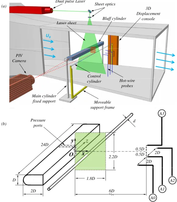
The experimental test facility is an Eiffel type, open-circuit wind tunnel. The tunnel is 8.835m long from the intake to the outlet. All segments of the wind tunnel have a square cross-section, similar to the intake shown in figure2.1(a). Only outlet has a circular cross-section since it houses the fan shown, in figure2.1(b). Figure2.1(c) shows the experimental area enclosed in a wooden chamber. The chamber dimensions are 2.03m × 1.56m × 1.5m, and it allows complete access to the experiment via doors on each side. These doors are closed and sealed during the wind tunnel activity, allowing the chamber to maintain constant pressure and temperature environment in and around the test section. Figure 2.1 also shows the test section (d), with some of its details: the main bluff cylinder (e), equipment for the control cylinder including the support frame (f) and the displacement consoles (g), pressure measurement electronics and tubing (h), and support and displacement equipment for the hot-wire probes (i). Depending on the experiment, the test section may contain imaging cameras for PIV acquisitions (not seen here), and mounted on the roof is an optical table (j) used for precise positioning of the laser sheet optics and mirrors (not shown). Complete layout and dimensions of the wind tunnel are given in the manufacturer’s technical drawing in figure2.2, and a more detailed description of the experimental geometry itself will be given in the next section.

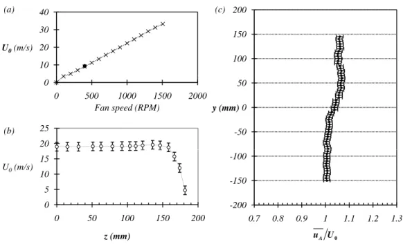
The wind tunnel is capable of producing speeds up to 33m/s; with less than 0.3% of tur-bulence intensity, and velocity homogeneity of ±0.4%. The velocity in the wind tunnel is set by controlling the revolutions of the electrical fan which is creating the under-pressure at the outlet, and are ranging from 0 to 1506 (RP M ). As a standard velocity of the experiments, we have selected the setting of 400 (RP M ). This setting gives a sufficiently high Reynolds number of the experiment, while allowing us to maintain reasonable seeding quality for the PIV measurements. Tunnel velocity a linear function of the revolutions per minute of the fan, and is given in the figure2.3(a), based on manufacturer’s specifications.

2. EXPERIMENTAL SETUP (a) (b) (c) (j) (e) (i) (d) (h) (g) (f)

2. EXPERIMENTAL SETUP 10 20 30 40 U0(m/s) (a) (c) 100 150 200 20 25 0 0 500 1000 1500 2000 Fan speed (RPM) (b) -50 0 50 y (mm) 0 5 10 15 0 50 100 150 200 U₀(m/s) -200 -150 -100 0.7 0.8 0.9 1 1.1 1.2 1.3 z (mm) uA U0

Figure 2.3: The wind tunnel velocity information: (a) manufacturers data on the mean ve-locity versus the control input; (b) experimentally measured spanwise veve-locity profile and (c) experimentally measured vertical velocity profile.

The test section has a square cross-section of 400mm × 400mm, with open sides. Its length, from the inlet to the outlet, is 960mm. The spanwise profile of velocity U (z) is shown in figure 2.3(b). We can see that the flow is uniform over a length of 300mm, after which the velocity decreases to zero on a typical length of 20mm. The vertical profile of velocity at 400rpm speed setting is shown in figure2.3(c). The streamwise velocity is changing by about 2.5% across the height of the test section, and it is slightly lower in the bottom part and slightly higher in the upper half of the tunnel. This is due to a temperature gradient in the air in front of the intake of the tunnel.

2.2

Experimental geometry

2.2.1

Main bluff cylinder

The primary cylinder (shown in figure2.4b) has a semi-circular leading edge which continues into a rectangular aft section, for a combined length of 2D = 50mm. The diameter of the semi-circle, and thus the height of the main cylinder, is D = 25mm. This is the characteristic length of the experiment, and will be used to define Reynolds and Strouhal numbers. It can be noted that contrary to slender bodies, for bluff bodies this height is much more important than the cord length, since it (among other factors) determines the size of the wake. Therefore,

this elongated ”D” shape has been chosen in order to have a constant height of the wake, for a wide range of Reynolds numbers. This requirement is fulfilled by the fact that the flow is detached at the blunt trailing edge, and that the shear layers are parallel before roll-up. This will be described in detail in section3.

As shown in figure2.4(a), the main cylinder is fixed at the edges of its span to the floor of the wind tunnel. The span of the body is S = 600mm. Therefore, in the spanwise direction, the edges of the main cylinder go beyond the width of the test section.

In the streamwise direction, the leading edge of the main cylinder is located at ≈ 1/5 of the test section length from the inlet. Vertically, it is exactly in the middle of the test section. Before each experiment, it is thoroughly verified that the span of bluff cylinder is parallel to the upper and lower wall of the test section, and also that it is at an angle of attack of α = 0◦ with regard to the incoming flow.

The main cylinder is made of metal, with highly polished surfaces. The inside is hollow, allowing access to ports for pressure measurements. The tubing that is connecting the ports to the measurements devices is running inside the cylinder, starting from both edges and finishing at the center section. As can be seen in figure2.4(b), the pressure measurement ports are located at the center span cross-section. Figure 2.5 shows in detail the number and distribution of pressure ports around the perimeter of the main cylinder center section. Each port is connected to the measurement device with a plastic tube of φ3mm and an average length of 1.5m ± 5cm.

2.2.2

Control cylinders

The requirements of the experiment dictate that the control cylinder needs to be moved easily between various positions downstream of the main cylinder. It is also imperative that while changing the position, the control cylinder doesn’t change its orientation relative to the main cylinder. Therefore, the control cylinder is connected by a rigid supporting frame to a displace-ment console. The supporting frame does not obstruct the flow, since it is located on the sides of the tunnel, outside of the steady flow, and below the tunnel floor. Some details of this setup can be seen in figure2.4(a).

The common span of all types of control cylinders used is s = 800mm. Due to different thickness and rigidity of the control cylinders, it was necessary to be able to stretch them in the spanwise direction, in order to eliminate slacking or vibrations. At the same time it was verified that the cylinders were not overstretched which could lead to deformations in the opposite sense. Additionally, absence of flow induced vibrations was verified visually, usually by the aid of a high speed camera used for the PIV acquisitions. Figure2.6shows the different cross-section shapes and sizes of the control cylinders.

The circular control cylinders were usually a metal wire of a specific diameter, except in the case of the d = 0.1mm cylinder, which was made out of a nylon string. The flat plate control cylinder is a metal plate of 1mm × 3mm, with slightly chamfered edges, the effect of which can be neglected. The experiments with the flat plate required a change in angle of attack of the

2. EXPERIMENTAL SETUP

Dual pulse Laser

3D Displacement console (a) Bluff cylinder Sheet optics console Laser sheet U₀ Bluff cylinder PIV Camera Control Moveable support frame cylinder Hot-wire probes Main cylinder fixed support d (b) Pressure _ports A3 support frame

z

O

x

y

Figure 2.4: Schematic representations of the wind tunnel test section and equipment layout (a) and the experimental apparatus in detail (b).

15° 3 6 4 5 7 8 9 10 11 12 13 14 2 15

Upper flat surface ports

4mm Base ports P(0) 4.5mm 15 1 2 27 26 25 24 23 22 21 20 15 16 17 18 19 31 28 30 29 32 27 26 25 24 23 22 21 20

Lower flat surface ports

Figure 2.5: locations, grouping and numbering of the pressure ports on the main cylinder.

flat plate. This was done visually, since there was no possibility of measuring accurately the angle of the plate. In addition to this, the plate itself was slightly undulated along its span, and all of this has to be taken into account when analyzing the results of these experiments.

2.2.3

Displacement of the control cylinder

The supporting frame of the control cylinder is connected to three Newport (M-)MTM long travel consoles, which are controlled by the Newport Motion Controller ESP301. These consoles are used to accurately position the control cylinder in Ox and Oy directions. The Oz direction hasn’t been used in our experiments, since both the main and secondary cylinders are 2D. The displacement console has accuracy better than 0.1mm.

The experiments are performed by moving the control cylinder through a set of pre-determined positions (xc, yc), and measuring local velocity in the wake and pressure distribution on the main

cylinder, for each position. The area of interest is shown in figure2.4(b) as the green rectan-gular area, which extends 1.8D downstream from the base of the bluff body, and ±1.1D above and below the horizontal axis of symmetry of the bluff body. The control cylinder is displaced in 0.04D (1mm) steps in the horizontal direction, and in 0.02D (0.5mm) steps in the vertical direction, except when noted otherwise. The origin (xc = 0,yc = 0) is defined as the intersection

between the horizontal axis of symmetry and the trailing edge of the bluff cylinder.

The movement sequence of the control cylinder is as follows: from the starting position (xc= 0,yc= −1.1D) the control cylinder is moved through 111 steps in the +Oy direction then

by 1 step in +Ox direction, continued by 111 steps in the −Oy direction and finally by 1 step in +Ox direction. This pattern is repeated so to cover the area of interest of 1.8D × 2.2D, with a resolution of 45 × 111 positions of the control cylinder. At each position, the control cylinder

2. EXPERIMENTAL SETUP 1mm 3 4mm 0 1 Circular control cylinders (d) 3mm 0.1mm 1mm Flat plate control

li d (h l) 3mm 1mm cylinder (h x l) α = 0° α = 45° α = 90° (Direction of flow)

Figure 2.6: Sizes and shapes of the control cylinders used in the experiments.

remains stationary, for a specified time interval, during which measurements are obtained. The whole experiment, taking into account short delays between the starting and stopping of the movement (for each step) and the measurements, lasts 48 hours.

When it is necessary to place the control cylinder at a single, specific position, it is done by placing it first at the origin, then moving it relatively from the origin position to the desired location. This ensures that the obtained location is not the absolute position in space with respect to the frame of the wind tunnel and the test section, but that it is accurate with respect to the exact position of the main cylinder, which is crucial. This was necessary because both the main cylinder and the control cylinders had to be dismantled and taken out frequently in order to make the wind tunnel available for other users.

2.3

Measurements and instrumentation

The experimental data presented in this thesis was obtained from three principal sources: hot-wire anemometry, differential pressure measurements and PIV acquisitions. The following sections will describe in detail the main measurement techniques and the post-processing of obtained data.

2.3.1

Local velocity measurements

Hot-wire measurements of local velocity in the wake is an accurate and unobtrusive way of recording the frequency of the global mode. The frequency is measured from the frequency of

the velocity fluctuations characteristic of the K´arm´an vortex street. The hot-wire probes are placed so that the passing of vortices from the vortex street is clearly registered.

Figure2.4(b) shows the placement of the four hot wire probes, marked A0 through A3, in the wake. The hot wire probes measure the modulus of local velocity in the xOy plane and will be denoted as uAi(t), where i refers to the label of the hot wire probe. They are all located at

x = 6D downstream of the trailing edge of the main cylinder, and at the same vertical level as its lower horizontal edge, at y = −0.5D, or its upper horizontal edge at y = +0.5D. In the spanwise direction, they are located at z = −2D, z = 0 and z = +2D. Not all of these positions have been used in every experiment. Therefore, for each presented experiment we will define the locations of the hot-wire probes for that particular instance, by referring to the labeling convention of Ai.

We use two DISA Type 55M10 and two DANTEC constant temperature anemometry units, connected to a PC with Labview software, as the control platform, to perform simultaneous acquisition of the signals. The hot-wire probes are DANTEC, and use an overheat ratio of 1.5. For more details about hot-wire anemometry theory please refer toLomas(1986).

The acquisition of each velocity signal is performed at a rate of 1kHz during the acquisition period tacq. The acquisition period is usually 30s or 60s. The power spectrum PuAi(f ) =

1 2π

R < uAi(t)uAi(t + τ ) >T exp(−2πif τ )dτ , computed from the velocity time series, is averaged over

a window of T = 4 seconds. Hence the frequency resolution of the spectra is ∆f = 0.25Hz. In order to find the frequency of the global mode, we use the peak detection subroutine, based on an algorithm that fits a quadratic polynomial to sequential groups of data points, where a group of points corresponds to a bandwidth of 10Hz. Strouhal number is the calculated as St = f D_U

0.

In order to characterize the 3D structure of the wake, spatial correlations are obtained from cross correlations between the local velocity measurements. The measurements of hot wire probes Ai are used to compute three spanwise correlation coefficients: r[0−1], r[1−2], r[0−2], and

a vertical correlation coefficient r[1−3] defined as:

r[i−j]=

u0_Aiu0_Aj q

u02_Ai u02_Aj

, (2.1)

where primes denote the fluctuating part of the velocity following the classical Reynolds de-composition X0(t) = X(t) − X. This notation will be used throughout the paper.

2.3.2

PIV measurements

Particle Image Velocimetry is used to visualize and obtain the velocity field around the bluff body and the control cylinder. A useful review of PIV principles and techniques may be found inAdrian (1991). Two separate PIV systems were used: a standard and a high-speed system. Both have been engaged into revealing the mean and fluctuating wake topology near the base

2. EXPERIMENTAL SETUP

of the main cylinder. The standard setup was also used in visualization experiments of the 3D properties of the wake in the horizontal plane (xOy) behind the main cylinder.

The standard system is comprised of a Litron LP4550, dual pulse 200mJ Nd:YAG laser, and a Lavision Imager PRO camera. The setup acquires images at a rate of 11Hz, and Lavision software DaVis 7 has been used to calculate the velocity fields. The vector calculation is done using single-pass, dual frame cross-correlation on constant window size. The interrogation window size is 32×32 pixels, and the entire image is 1600×1400 pixels. The time delay between the two frames is 75µs, for both experiments. Each acquisition records 200 image pairs.

The Hi-speed system uses a Pegasus dual pulse laser with a wavelength of 527nm and output energy of 10mJ , with a pulse rate of up to 20, 000Hz. A Photron Fastcam high speed camera is used for imaging, with an acquisition rate of 3, 000Hz at 1024 × 1024 pixel resolution. A special version of DaVis 7 is used to process high speed PIV data. Standard acquisition is 500 image pairs, at a rate of 3, 000Hz. The image sizes are 768 × 480 pixels in the case of the d = 4mm experiment, and 640 × 368 pixels for the d = 3mm experiment. The vector calculation is done using multi-pass, dual frame cross-correlation on changing window size. The interrogation window size is changing from 128 × 128 pixels to 16 × 16 pixels, with a 50% overlap.

The data from our PIV measurements will be presented in the form of: i) component of mean velocity in Ox direction, u(x, y), ii) mean vorticity component in xOy plane, ωz(x, y) =

(∂v ∂x−

∂u

∂y), and iii) Reynolds Stress components v02(x, y) and u0v0(x, y).

We will use u(x, y) to measure the length of the recirculation bubble Lb/D as the horizontal

distance from the trailing edge, of the main cylinder, to the point where the iso-contour of u = 0 intersects Ox. The uncertainty of the Lb/D is measured manually from stagnation point

definition of the velocity field streamlines.

Phase-averaged flows

From the instantaneous flow fields of PIV measurements, we can obtain phase averaged flows (seePerrin et al.,2007). This technique allows us to observe the flow dynamics at the frequency of the global mode, without noise of other scales typical of turbulent flows. One position in the vector field is chosen as a reference point, and the velocity time series are extracted for that point for the duration of the entire acquisition. The resulting time series are processed through bandpass filter, shown in figure 2.7(a), and are used to make a time basis for the averaging. The reference point is usually chosen at a point, in the flow, where the K´arm´an street vortices can be clearly seen, and the each phase is well resolved. Using a Hilbert transform, we are separating the velocity signal from the time series into amplitude and phase which is shown in figure2.7(b). The Hilbert transform is obtained by performing a Fast Fourier Transform (FFT) on our velocity signal, removing half of the obtained data, and then performing an inverse FFT on the remaining signal. The FFT and inverse FFT transformations have been performed using the appropriate modules in LabView software. From the extracted phase signal, we can choose a phase, and perform averaging of velocities in all other points in the flow, on the same basis,

4 0 4 8 v (m/s) a) -8 -4 0 100 200 300 400 500 t (frames)

Raw signal Filtered signal

2 0 2 4 θ g g b) -4 -2 0 50 100 150 200 250 300 350 400 450 500 t (frames)

Figure 2.7: Local transversal velocity v(t) from instantaneous high-speed PIV fields, used to build the phase-averaged signal: (a) raw (red) and filtered (black) velocity signal and (b) phase θ(t) of the velocity signal.

i.e. on the same phase. Since vorticity in two dimension acts as a scalar it is simple to calculate and is the most convenient form of result presentation, in our case.

2.3.3

Pressure measurements

The main cylinder is equipped with 32 pressure taps (figure2.4b and figure2.5), distributed along the entire perimeter of its cross-section at mid-span (z = 0). They are connected to two Scanivalve DSA 3217/16px differential pressure measurement arrays, capable of taking 100 samples of pressure per second. These samples are automatically averaged and a mean pressure is given as an output. In our mapping experiments, we have performed 30s and 40s long measurements of pressure for each position of the control cylinder. From these measurements, we obtain a mean pressure coefficient Cp(s):

Cp(s) =

p(s) − pref

p(0) − pref

, (2.2)

where pref is a reference static pressure, measured at the inlet of the wind tunnel test area,

2. EXPERIMENTAL SETUP

thesis, we will refer to the pressure in arbitrary units (A.U.), which is an unscaled unit given by the output of the Scanivalve devices, where 100A.U. = 9.7P a.

In our study, we take into account only the pressure drag, since the Reynolds numbers of this magnitude and the shape of the main cylinder render the viscous drag contribution to the drag coefficient to be negligible. The total drag can be given as Cd = Cd(p)+ Cd(ν); since the

flow around our main cylinder is strongly separated, the pressure part of the drag has an order of magnitude O(1) and the viscous part O(_√1

Re) (Batchelor, 1967). The viscous drag surely

is changed by the control cylinder, but this change is negligible compared to the changes in pressure drag, for the Reynolds numbers investigated in this work. The sectional form drag Cd is then classically estimated by integrating the projected pressure stress over the cylinder

perimeter, as in: Cd= 1 D I Cp(s)~n · ~exds. (2.3)

The lift is computed by integrating the y component of pressure:

Cl=

1 D

I

Cp(s)~n · ~eyds. (2.4)

The base pressure coefficient Cpb is computed from the spatial average of the 5 pressure taps

that are distributed on the blunt base of the cylinder:

Cpb= 1 D Z base Cp(s)ds. (2.5)

The DSA devices are not able to recover the true rate of fluctuation of the pressure, but we can still build the Cpb(rms)from those 40s of measurements, which gives an image of the fluctuation

levels.

2.4

Experimental problems

Two main difficulties were encountered during the long mapping experiments: variations of the environment temperature and the asymmetry of the flow around the main cylinder. Next two sections will describe and discuss both effects in detail.

2.4.1

Ambient temperature variations

In order to investigate this occurrence which has plagued more or less each of our experiments, we have performed an experiment in which we measured the pressure around the bluff cylinder, for the duration of a typical mapping experiment, except that there was no control cylinder present in the wake, and no velocity in the tunnel (U0 = 0). The goal was simply to see how

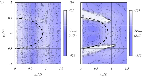
does the pressure change purely with time. The results are presented in figure 2.8(a) for the pressure at the head of the main cylinder and in (b) for the pressure at the base. The definitions

0.5 1 0.5 1 (a) (b) 18 23 -0.5 0 yc / D -0.5 0 yc / D 0 Δp_base (A.U.) 0 Δphead (A.U.) -1 0 0.5 1 1.5 x_c/ D -1 0 0.5 1 1.5 x_c/ D 0 0

Figure 2.8: Maps of the ambient variations of (a) pressure at the head and (b) pressure at the base of the main cylinder, when no control cylinder is present and the velocity is U0 = 0.

Pressure is given in arbitrary units (see section2.3.3). for these are given by equations2.6and2.7:

∆phead= p(i = 0) − pref, (2.6)

∆pbase= 1 5 19 X i=15 p(i) − pref, (2.7)

where index i denotes the pressure port as per numbering given in figure2.5. The pressure here is presented in arbitrary units, which we will refer to simply as ”units” in further text.

If we plot the pressure in these two maps on an absolute time scale we obtain figure 2.9. Here we can see a time span of the experiment to be roughly two days, starting at 14h on day 1 and ending at 12h on day 3. We see pressure increase until midnight between day 1 and day 2, then slight decrease during the morning hours of day 2, followed by sharp increase in the afternoon period and again a plateau in the evening to midnight. Morning hours of day 3 again see a decrease in pressure. Based on the above, we can conclude that the pressure variation is closely correlated with the time of day, ie. with the daily temperature variations. Months of April and May can be very hot during the day and very cold during the night, and this drastic change has left its imprint on our experiment.

We can observe actually two types of pressure variations: one is described above and is of the order of 20 units, but another is the difference between the pressure at the head and at the base when there is no velocity in the tunnel, and when this pressure difference should be

2. EXPERIMENTAL SETUP 10 15 20 25 Pressure (a.u.) 0 5 0 24 48 72 Time (h)

Figure 2.9: Evolution in time of pressure at the head of the main cylinder (black) and at the base (grey), when no control cylinder is present and the velocity is U0= 0. Pressure is given in

arbitrary units (see section2.3.3).

constant. This is clearly visible in figure 2.9; both pressures start at 0, but as time evolves, the pressures diverge and we can see a drift of about 5 units, between these two measurements. This pressure drift is probably caused by the Scanivalve devices.

In order to quantify the significance of these variations, we need to compare them with normal working conditions for the mapping experiments. As a reference, the pressure in arbi-trary units for the natural flow at Re = 13, 000 is phead ≈ 447 and pbase ≈ 275. Therefore,

the ambient pressure variations are at most around 7% of the natural values for the standard mapping experiment. This poses a serious difficulty when smaller control cylinders of 0.1mm and 1mm are used, since the variations are of the same order as some of the effects of those control cylinder. However, the variation occurs in good correlation with the time of day, and is relatively easy to filter out from the resulting map. The variation caused by the Scanivalve devices is on the order of 1%, and poses no significant impact on our results.

2.4.2

Shear layer asymmetry

If one looks at figure 3.2, it is clear after a careful check that the the pressure distribution for the natural flow around the main cylinder is not exactly symmetric with regard to the Ox axis. There are many small imperfections in our experimental setup who influence this; starting from the air that is entering the inlet of the tunnel up to the setup of zero inclination of the bluff cylinder, which is done by hand and level. The lift maps in many experiments which will be presented in further text betray this asymmetry by the fact that the natural lift is always slightly biased. However, usual lift bias and pressure asymmetry is not big enough to significantly change the results. We have performed many experiments and find that the structure of the sensitive regions is very robust. If we compare the maps of base pressure for the 3mm circular control cylinder in figures 4.3(b) and 4.9(b) we can see an obvious difference in the shapes, but all of the different regions of pressure sensitivity are present in both examples.

Chapter 3

Natural flow around the bluff

cylinder

3.1

Boundary layer evolution

We will first describe the basic properties of the ”natural” flow around the main cylinder (when no control cylinder is present). The immediate question is: how does the boundary layer evolve along the surface of the main cylinder, for a wide range of Reynolds numbers around the one used in our experiments? The free stream velocity of is measured at the inlet of the tunnel test area, and the Reynolds number is calculated, with the main cylinder height D as the characteristic length, as Re = DU0

ν . We have used PIV acquisitions to obtain mean

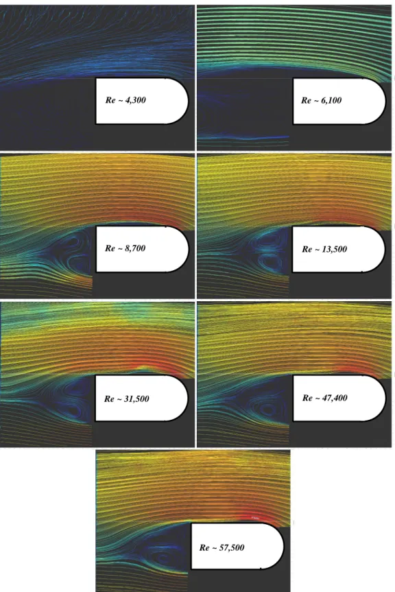
velocity fields for several different Reynolds numbers and the resulting velocity streamlines can be observed in figure3.1. First, we see a laminar flow for Re = 4300 with no detachment; the flow speed is very low and the PIV imaging was barely adequate to resolve the streamlines, but it is apparent that there is no flow detachment until the trailing edge. For a Re = 6100 we can see that the boundary layer is detached at the junction between the semi-circular front and the upper flat surface. Flow visualization (not shown here) reveals that the detached shear layer stays laminar for some distance after the detachment and never re-attaches, producing a wide wake. For Re = 8700 the shear layer undergoes a transition to turbulent and starts to re-attach at the trailing edge of the main cylinder. Since the transition to turbulence of the detached boundary layer occurs progressively earlier when we increase from Re = 13500 to Re = 57500, we can observe how the detachment bubble gets smaller and the re-attachment point moves upstream. So, from a detachment bubble that covers the entire length of the main cylinder’s flat surface, for Re = 8700, we arrive at a very small bubble that would ultimately disappear if we could increase Re further. This case is not shown here, but it would have a completely attached, fully turbulent boundary layer. The pressure distribution around the main cylinder at different Reynolds numbers is shown in figure3.2. We can observe that the pressure

3. NATURAL FLOW AROUND THE BLUFF CYLINDER

coefficient is constant at the front of the main cylinder, and slightly affected near the junctions with the upper and lower flat part. The level of the base pressure is changing with the Re, and this change is approximately uniform for all five base pressure ports. The radical change in the pressure distribution on the upper and lower flat surfaces confirms the PIV images of the boundary layer change, shown earlier.

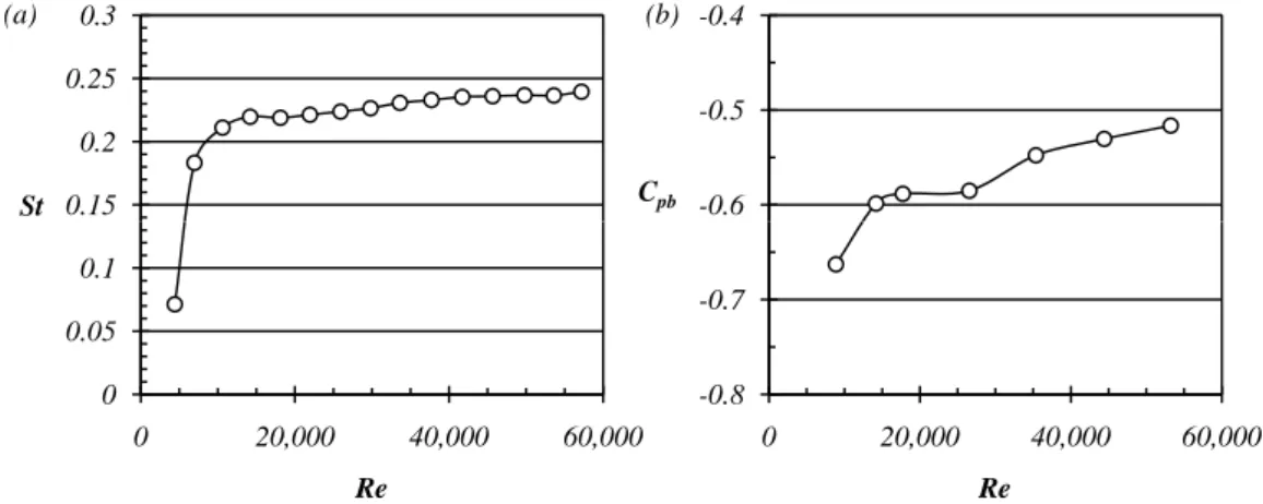
Figure3.3(a) shows how the natural Strouhal number changes when we change the Reynolds number of the experiment. The relationship between the Reynolds number and the vortex shedding frequency is consistent with the work for a similarly shaped bluff cylinder by Rowe et al. (2001). This is not the case with the base pressure which in our case is also increased with increasing Re as can be seen in figures3.2and3.3(b).

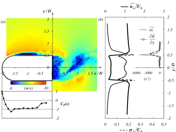
The standard flow conditions of the experiment are defined by a free stream velocity of U0 = 8m/s, and the Reynolds number is calculated to be Re = 13000. These conditions are

used for all of the experiments, except where noted differently. Figure 3.4 summarizes the main properties of the natural flow at Re = 13000. The color map in Figure3.4(a) shows the instantaneous modulus of velocity obtained from PIV acquisitions at z = 0. The boundary layer, that is initiated at the stagnation point x = −2D separates at the junction with the flat wall at x = −1.5D. The laminar separation becomes turbulent, as shown by the presence of periodic regions of high velocities in Figure3.4(a), revealing a transition mechanism due to the Kelvin-Helmholtz instability. The detached boundary layer re-attaches at about x = −0.4D. The turbulent boundary layer finally breaks away at the sharp trailing edge x = 0 of the main body. From hot-wire probe measurements of the boundary layer, at x = −0.1mm, just upstream of the trailing edge (shown in figure3.5), we have obtained a boundary layer thickness of δ99 = 0.12, momentum deficit thickness of δ2 = 0.014 and the form factor of H12 = 1.24.

The boundary layer properties are similar to the compiled results in the recent work ofPastoor et al. (2008) involving blunt trailing edge cylinders. However, the base pressure in our case Cpbn= −0.60, is lower compared to previous studies (−0.57 to −0.51). The difference might be

attributed to end conditions, that are free in our case and bounded by walls in Pastoor et al.

(2008). The form drag computed from equation (2.3) is Cdn= 0.74.

The properties of the turbulent mixing layers just after the detachment from the trailing edge are analyzed using flying hot wire measurements performed at x = 0.1mm and traversed in the vertical direction through −2D < y < +2D (in steps of 0.02D). The curves in figure3.4(b) show the mean velocity profile, uA (thick black line); and the fluctuation profile, σ =

q u02

A

(dashed line). The maximum fluctuation rate in the mixing layer is 25%. The turbulent mixing layer thickness δ1/2 can be deduced from the vertical gradient of the mean velocity∂u∂yA.

This gradient is shown, as thin black line, in the inset of Figure 3.4(b). Defining δ1/2 as the

width of the velocity gradient peak at half of its height, we find a turbulent layer thickness of δ1/2 = 0.05D = 1.25mm. The vertical component of the velocity being negligible at the

trailing edge, the mean velocity gradient there is also a good estimate of the mean vorticity:

∂uA

Re ~ 4,300 Re ~ 6,100

Re ~ 8,700 Re ~ 13,500

Re ~ 31,500 Re ~ 47,400

Re ~ 57,500

Figure 3.1: Streamlines of the mean velocity for the natural flow around the main cylinder for different Re.

3. NATURAL FLOW AROUND THE BLUFF CYLINDER 0.5 1 upper flat surface base front up front down lower flat surface Reynolds number -0.5 0 Cp 8865 14184 17730 26543 35372 number -1.5 -1 0 0.2 0.4 0.6 0.8 1 35372 44415 53245 s / L

Figure 3.2: Pressure coefficient Cp(s) distribution around the perimeter of the main cylinder

for different Re.

0.15 0.2 0.25 0.3 St (a) (b) -0.6 -0.5 -0.4 Cpb 0 0.05 0.1 0 20,000 40,000 60,000 -0.8 -0.7 0 20,000 40,000 60,000 Re Re

Figure 3.3: Evolution of (a) Strouhal number St and (b) base pressure coefficient Cpb of the

2 0 1 2 3 (a) (b) 0

U

u



U



Figure 3.4: Natural flow around the bluff body at Re = 13000; the color map (a) shows an instantaneous field of the modulus√u2_{+ v}2_{, with velocities ranging from 0m/s for black, up}

to 10m/s for orange, with the Cp(s) distribution shown below. The diagram on the right (b)

depicts the vertical profile measured with the flying hot wire just behind the rear of the blunt body at x = 0.1mm. The mean uA (thick line) and the fluctuation σ of velocity (dashed line)

are normalized by U0. The inset diagram in (b) is a plot of the vorticity ωz measured from

PIV (circles), and estimated (see text) from local velocity measurements (thin line). The plot shares the primary y/D axis.

3. NATURAL FLOW AROUND THE BLUFF CYLINDER 0 0.05 0.1 0.15 0.2 2 0 U A σ 1 1.5 y / D 0 0.5 0 0.5 1 1.5 2 2.5 3 0

U

u

Figure 3.5: Boundary layer for Re = 13000 at x = −0.1mm, just before detachment from the trailing edge. Mean velocity uA (thick line) and the fluctuation of velocity σA(dashed line) are

figure3.4(b). If we compare the two curves in the inset, we can see that the PIV interrogation window, with its size of 0.04D × 0.04D, induces a clear coarse graining effect, which has to be taken into account while analyzing the PIV results that will be presented in the following sections.

3.2

The mean natural wake and the dynamics in the wake

Now that we have described the flow in the vicinity of the body, we turn to some properties of the wake. The mean wake consists of a recirculation bubble, which is a region of reversed flow, and is shown in figure3.6(a). The recirculation bubble is bounded by the two detached turbulent shear layers described above, and the vortex formation region produced by the shear layers roll-up. The detached shear layers are nicely visualized by the contours of z component of mean vorticity ωz in figure3.6(b). A characteristic size of the formation region is the mean

bubble length, measured to be Lbn/D = 0.82 ± 0.04 in the case of the natural flow.

The wake dynamics are dominated by a global mode, known as the K´arm´an vortex street. The detached shear layers roll up and meet each other at a characteristic distance downstream from the trailing edge of the main cylinder, and vortex are shed at a selected frequency. The PIV measurements of Reynolds stresses in the natural wake, shown in figure3.6(c) and (d), give a good reference of the dynamic part of the wake. We can observe one maximum of v02_,

and a maximum and a minimum for u0_v0_{. These extrema are located at the points in the wake}

where the global mode originates, as we will see in later chapters. For now, we should note the streamwise locations of the extrema as X_v02

M ax, Xu0v0M ax and Xu0v0M in and the streamwise size of the first contour around each extrema, marked as δ_v02 and δ_u0_v0. A detailed analysis of how these values are affected by the control cylinders will be shown in chapter4.

The global mode frequency is clearly observed in Figure3.7, where the local spectra, from four hot wire probes, all display the peak in amplitude around the same frequency. This is identified as the natural frequency of fn = 70.75 ± 0.25Hz, at the Re = 13000. The natural

Strouhal number is calculated as St = 0.221. The large width of the peaks are related to the three dimensional disturbances of the turbulent wake, such as oblique vortex shedding and vortex dislocations (Prasad & Williamson,1997;Williamson,1996a). Between the three spectra obtained at different spanwise locations, we can observe slight differences: the peaks of the two centerline wires (A1 and A3) have larger amplitude, and better definitions. The peak of the first harmonic are better seen in the spectra of the wires on the right (A0) and left (A2) of the centerline. The differences in the peak definition are also indicating 3D properties of the wake, partly induced by the ends effect. The similarity of the spectra (A2) and (A0) is a consequence of the experimental symmetry with respect to the central plane z = 0.

The correlation coefficient values computed from Eq.2.1 for the natural case are rn[0−1] =

0.204, rn[1−2] = 0.190, rn[0−2] = 0.089 and rn[1−3] = −0.31. Three-dimensionality disturbances

3. NATURAL FLOW AROUND THE BLUFF CYLINDER (a) (b)

X

X

Figure 3.6: Mean and dynamic components of the natural wake: (a) mean streamwise veloc-ity u, with continuous lines for positive and dashed lines for negative values, from the list [−3, −2, −1, −0.5, 0, 0.5, 1, 2...8]m/s; (b) mean vorticity ωz, where lines are at ±500, ±1000 and

±1500s−1_{(continuous for positive, and dashed for negative vorticity) and Reynolds stress}

com-ponents (c) v02_{, in range of 0(m/s)}2 _{to 15(m/s)}2 _{and (d) u}0_v0_{, in range of ±5(m/s)}2 _{(b). The}

isolines are in the interval of 1(m/s)2 _{(continuous lines for positive and dashed for negative}

500 5000 50000 A3 A2 A1 5 50 PuAi(f) A0 1 5 50 500 f (Hz)

Figure 3.7: The power spectra of the velocity signals for the natural flow measured at the three spanwise locations (see figure2.4b). Starting from A0, each subsequent spectrum is shifted by a decade, for visibility purposes.

values of rn[0−1] and rn[1−2], performed on a distance 2D, on either side of the wake centerline,

are quite similar. Once again, this is a consequence of the experimental symmetry with respect to the centerplane z = 0. For the spanwise distance of 4D, the correlation coefficient rn[0−2] is

Chapter 4

Wake with a circular control

cylinder

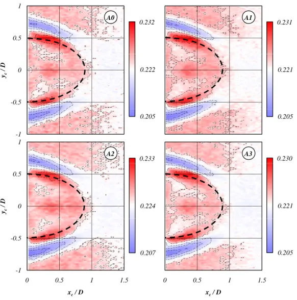
In the following sections, we will present the results of experiments when a small circular control cylinder is placed in the wake. Two diameters of control cylinder will be tested, the control cylinder of diameter d = 1mm, which is always smaller than the mixing layer thickness at the trailing edge detachment (see chapter3). The other control cylinder diameter is d = 3mm. We will show the maps of sensitivity of the wake for both control cylinders, as well as focus in detail on what happens when a control cylinder is displaced vertically across the wake at a chosen downstream distance from the main cylinder, as well as when it is placed at some key positions on the horizontal axis of the wake.

4.1

Mapping of global properties

4.1.1

Global frequency change

If we assemble the detected global mode frequency (see section2.3.1) for each position of the control cylinder (see section 2.2.3), we obtain a map of the sensitivity for the global mode frequency to the presence of the control cylinder, as shown in figure4.1for d = 1mm, and in figure4.2 for d = 3mm. The selected global mode frequency is represented as the Strouhal number, with the natural frequency for each map depicted in white. We present four maps for each control cylinder size, obtained from the four hot-wire probes placed in the wake. We can confirm that the detected frequency is changing in an identical fashion all along the span of the main cylinder, because there are no noticeable differences in structure if we compare the appropriate maps between probes A0, A1 and A2. This is true for both 1mm and 3mm control cylinders. Also, maps for wires A1 and A3 are identical, which is expected from the vertical symmetry of the K´arm´an vortex street (see positions of wires A1 and A3 in figure 2.4). We