Unsupervised representation learning for anomaly detection on neuroimaging. Application to epilepsy lesion detection on brain MRI

(1)

HAL Id: tel-02062210

https://hal.archives-ouvertes.fr/tel-02062210v2

Submitted on 17 Jul 2019

HAL is a multi-disciplinary open access

archive for the deposit and dissemination of sci-entific research documents, whether they are pub-lished or not. The documents may come from teaching and research institutions in France or abroad, or from public or private research centers.

L’archive ouverte pluridisciplinaire HAL, est destinée au dépôt et à la diffusion de documents scientifiques de niveau recherche, publiés ou non, émanant des établissements d’enseignement et de recherche français ou étrangers, des laboratoires publics ou privés.

detection on neuroimaging. Application to epilepsy

lesion detection on brain MRI

Zaruhi Alaverdyan

To cite this version:

Zaruhi Alaverdyan. Unsupervised representation learning for anomaly detection on neuroimaging. Application to epilepsy lesion detection on brain MRI. Medical Imaging. Université de Lyon, 2019. English. �NNT : 2019LYSEI005�. �tel-02062210v2�

(2)

N°d’ordre NNT : 2019LYSEI005

THESE de DOCTORAT DE L’UNIVERSITE DE LYON

opérée au sein de

Centre de Recherche en Acquisition et Traitement de l'Image

pour la Sant

é (CREATIS)

Ecole Doctorale

N° 160

(Electronique, Electrotechnique, Automatique)

Spécialité de doctorat

:

Traitement du Signal et de l'image

Soutenue publiquement le 18/01/2019, par :

Zaruhi ALAVERDYAN

Unsupervised representation learning

for anomaly detection on

neuroimaging. Application to epilepsy

lesion detection on brain MRI

Devant le jury composé de :

Cardoso, Jorge M. Professeur des Universités King's College London Rapporteur

Mateus, Diana Professeur des Universités Ecole Centrale Nantes Rapporteure

Bonnet-Loosli, Gaëlle Maître de Conférences Université Clermont Auvergne Examinatrice

Fromont, Elisa Professeur des Universités Université de Rennes 1 Examinatrice

Jung, Julien Praticien Hospitalier CHU de Lyon Examinateur

Lartizien, Carole Directrice de recherche CNRS Directrice de thèse

(3)

SIGLE ECOLE DOCTORALE NOM ET COORDONNEES DU RESPONSABLE

CHIMIE CHIMIE DE LYON http://www.edchimie-lyon.fr

Sec. : Renée EL MELHEM Bât. Blaise PASCAL, 3e étage

[email protected]

INSA : R. GOURDON

M. Stéphane DANIELE

Institut de recherches sur la catalyse et l’environnement de Lyon IRCELYON-UMR 5256

Équipe CDFA

2 Avenue Albert EINSTEIN 69 626 Villeurbanne CEDEX [email protected] E.E.A. ÉLECTRONIQUE, ÉLECTROTECHNIQUE, AUTOMATIQUE http://edeea.ec-lyon.fr Sec. : M.C. HAVGOUDOUKIAN [email protected] M. Gérard SCORLETTI École Centrale de Lyon

36 Avenue Guy DE COLLONGUE 69 134 Écully

Tél : 04.72.18.60.97 Fax 04.78.43.37.17

E2M2 ÉVOLUTION, ÉCOSYSTÈME,

MICROBIOLOGIE, MODÉLISATION

http://e2m2.universite-lyon.fr

Sec. : Sylvie ROBERJOT Bât. Atrium, UCB Lyon 1 Tél : 04.72.44.83.62 INSA : H. CHARLES

M. Philippe NORMAND

UMR 5557 Lab. d’Ecologie Microbienne Université Claude Bernard Lyon 1 Bâtiment Mendel 43, boulevard du 11 Novembre 1918 69 622 Villeurbanne CEDEX [email protected] EDISS INTERDISCIPLINAIRE SCIENCES-SANTÉ http://www.ediss-lyon.fr

Sec. : Sylvie ROBERJOT Bât. Atrium, UCB Lyon 1 Tél : 04.72.44.83.62 INSA : M. LAGARDE

Mme Emmanuelle CANET-SOULAS INSERM U1060, CarMeN lab, Univ. Lyon 1 Bâtiment IMBL

11 Avenue Jean CAPELLE INSA de Lyon 69 621 Villeurbanne Tél : 04.72.68.49.09 Fax : 04.72.68.49.16 [email protected] INFOMATHS INFORMATIQUE ET MATHÉMATIQUES http://edinfomaths.universite-lyon.fr

Sec. : Renée EL MELHEM Bât. Blaise PASCAL, 3e étage

Tél : 04.72.43.80.46 Fax : 04.72.43.16.87 [email protected] M. Luca ZAMBONI Bât. Braconnier 43 Boulevard du 11 novembre 1918 69 622 Villeurbanne CEDEX Tél : 04.26.23.45.52 [email protected]

Matériaux MATÉRIAUX DE LYON

http://ed34.universite-lyon.fr

Sec. : Marion COMBE

Tél : 04.72.43.71.70 Fax : 04.72.43.87.12 Bât. Direction [email protected] M. Jean-Yves BUFFIÈRE INSA de Lyon MATEIS - Bât. Saint-Exupéry 7 Avenue Jean CAPELLE 69 621 Villeurbanne CEDEX

Tél : 04.72.43.71.70 Fax : 04.72.43.85.28

MEGA MÉCANIQUE, ÉNERGÉTIQUE,

GÉNIE CIVIL, ACOUSTIQUE

http://edmega.universite-lyon.fr

Sec. : Marion COMBE

Tél : 04.72.43.71.70 Fax : 04.72.43.87.12 Bât. Direction [email protected] M. Jocelyn BONJOUR INSA de Lyon Laboratoire CETHIL Bâtiment Sadi-Carnot 9, rue de la Physique 69 621 Villeurbanne CEDEX [email protected] ScSo ScSo* http://ed483.univ-lyon2.fr

Sec. : Viviane POLSINELLI Brigitte DUBOIS

INSA : J.Y. TOUSSAINT Tél : 04.78.69.72.76 M. Christian MONTES Université Lyon 2 86 Rue Pasteur 69 365 Lyon CEDEX 07 [email protected]

(4)

Մերոնց․

(5)

(6)

Acknowledgements

I would first like to thank my PhD supervisor, Carole Lartizien, for starting this project and allowing me to become a part of it. It has been an ambitious endeavour and this work reflects only a part of the efforts we have invested.

I would also like to thank all the people who, voluntarily or not, shaped my experience of the past 3 years. Mo, Meriem and Younes, thanks for welcoming me, showing me around and tailoring my expectations of what was going to come next. Thanks to Robert, for introducing many important ideas into my life and Tiago, for all the music, dances and nice moments we shared. Aneline, Sami, Yuemeng, Maxime and Vincent, I thank you all for the countless jokes and foolishness which made my last days in Lyon so memorable. Special thanks to Emeline, for all the support you gave me and for the fun we had. Nina and Kenny, well, you know ... I am deeply thankful to my dear mexicans, Pavel, for lifting my spirits and putting up with all the whining, and Manuel, simply for being the best.

Finally, I would like to thank all those who, despite being miles away, are of the utmost importance to me. I thank my parents and my dear sister, for their blind faith in me and the unconditional support. My friends, Anka, Arpy and Hrant, for reminding me of the good times every time we talked.

Having all of you in my life is perhaps the best luck of all.

(7)

(8)

Abstract

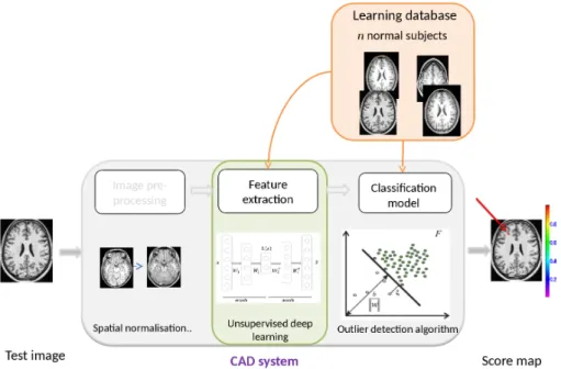
Epilepsy affects around 50 million people worldwide, a third of those diag-nosed with medically refractory epilepsy where seizures cannot be controlled by pharmacotherapy. For such patients, surgical resection of the epileptogenic zone may offer a seizure-free life. The success of such surgeries largely depends on the accuracy of the epileptogenic zone localization. Neuroimaging, including magnetic resonance imaging (MRI) and positron emission tomography (PET), has been increasingly considered in the pre-surgical examination routine. This work represents one attempt to develop a computer aided diagnosis sys-tem for epileptogenic lesion detection based on neuroimaging data, in particular T1-weighted and FLAIR MR sequences. Given the complexity of the task and the lack of a representative voxel-level labeled data set, the adopted approach, first introduced in [El Azami et al., 2016], consists in casting the lesion de-tection task as a per-voxel outlier dede-tection problem. The system is based on training a one-class SVM model for each voxel in the brain on a set of healthy controls, so as to model the normality of the voxel. For an unseen patient, each voxel is assessed against the corresponding one-class SVM model which yields a signed score of its anomalousness. Anomalous lesions can hence be found as local neighborhoods of voxels with low scores.

The main focus of this work is to design representation learning mechanisms, capturing the most discriminant information from multimodality imaging. Man-ual features, designed to mimic the characteristics of certain epilepsy lesions, such as focal cortical dysplasia (FCD), on neuroimaging data, are tailored to individual pathologies and cannot discriminate a large range of epilepsy lesions. Such features reflect the known characteristics of lesion appearance; however, they might not be the most optimal ones for the task at hand. Our first con-tribution consists in proposing various unsupervised neural architectures as potential feature extracting mechanisms and, eventually, introducing a novel configuration of siamese networks, to be plugged into the outlier detection con-text. The proposed system, evaluated on a set of T1-weighted MRI of epilepsy patients, showed a promising performance but a room for improvement as well. To this end, we considered extending the CAD system so as to accommodate multimodality data which offers complementary information on the problem at hand. Our second contribution, therefore, consists in proposing strategies to combine representations of different imaging modalities into a single framework for anomaly detection. The extended system showed a significant improvement on the task of epilepsy lesion detection on T1-weighted and FLAIR images. Our last contribution focuses on the integration of PET data into the system. An obstacle encountered often in medical applications is the small number of subjects with the full set of imaging modalities. This limits the performance of a system when the subjects with missing data are discarded. We therefore delve into strategies of synthesizing PET data from the corresponding MRI ac-quisitions and show an improved performance of the system when synthesized images are used in addition to the real ones.

(9)

(10)

Résumé étendu

Environ 50 million personnes souffrent d’une épilepsie partielle, dont un tiers atteint d’une épilepsie réfractaire à tous les médicaments. La chirurgie, qui con-stitue aujourd’hui le meilleur recours therapeutique, nécessite un bilan préopéra-toire complexe. L’analyse de données d’imagerie telles que l’imagerie par réso-nance magnétique (IRM) anatomique et la tomographie d’émission de positons (TEP) au FDG (fluorodésoxyglucose) tend à prendre une place croissante dans ce protocole, et pourrait à terme limiter les recours à l’électroencéphalographie intracérébrale (SEEG), procédure très invasive mais qui constitue encore la technique de référence.

Cette étude vise à développer un système d’aide au diagnostic (CAD) pour le détection de lésions épileptogènes, reposant sur l’analyse de données de neu-roimagerie, notamment, l’IRM T1 et FLAIR. Etant donné la complexité du problème et le manque d’une base de données, annotée à l’échelle de voxel, représentative de la pathologie, l’approche adoptée, introduite précédemment par [El Azami et al., 2016], consiste à placer la tâche de détection dans le cadre de la détection du changement à l’échelle du voxel. Le système est basé sur l’apprentissage d’un modèle one-class SVM pour chaque voxel dans le cerveau, en utilisant un ensemble de sujets sains, dont le but est de modéliser la nor-malité du voxel. Pour un patient donné, chaque voxel est évalué par le modèle oc-SVM, correspondant à sa localization spatiale, et ce dernier produit une valeur numérique signée, représentant l’anormalité du voxel. Les lésions anor-males peuvent ensuite s’identifier comme des voisinages de voxels, ayant des valeurs très négatives.

L’objectif principal de ce travail est de développer des mécanismes d’apprentissage de représentations, qui capturent les informations les plus discriminantes à par-tir de l’imagerie multimodale. Les caractéristiques manuelles, conçues pour imiter les caractéristiques de certaines lésions épileptogènes sur la neuroim-agerie, notamment les dysplasies corticales focales (FCD), sont spécifiques aux pathologies individuelles et n’ont pas la capacité de discriminer un ensemble varié de lésions épileptogènes. Ce type de caractéristiques reflète la connais-sance existante sur l’apparence de lésions. Par contre, elles ne sont pas for-cément les plus pertinentes pour la tâche visée. Notre première contribution porte sur l’intégration de différents réseaux profonds non-supervisés, en tant que mécanismes d’extraction de caractéristiques, dans le cadre du probleme de detection de changement. Eventuellement, nous introduisons une nouvelle configuration des réseaux siamois, mieux adapté à ce contexte. Le système CAD proposé a été évalué sur l’ensemble d’images T1 IRM des patients at-teint d’épilepsie. Nous avons démontré une performance importante qui reste, tout de même, à améliorer. Pour cela, nous avons considéré d’étendre le sys-tème pour intégrer des données multimodales qui possèdent des informations complémentaires sur la pathologie en question. Notre deuxième contribution, donc, consiste à proposer des stratégies de combinaison des différentes modal-ités d’imagerie dans un système pour la détection des changements. Ce système

(11)

Notre dernière contribution se focalise sur l’intégration des données PET dans le système proposé. Très souvent, dans les applications médicales, le nombre de sujets ayant les acquisitions de toutes les modalités envisagées, est assez limité. La performance des systèmes, où l’on ne considère que les sujets ayant toutes les acquisitions, est souvent faible. Pour cette raison, nous envisageons de synthétiser les données manquantes à partir des images des autres modalités présentes. Nous essayons, donc, de générer des images TEP en se servant des images IRM disponibles. Nous démontrons que le système entraîné sur les don-nées réelles et synthétiques présente une amélioration importante par rapport au système entraîné sur les images réelles uniquement.

(12)

General introduction

Epilepsy is a common neurological disorder affecting around 50 million people worldwide according to the World Health Organization (WHO). It is characterized by an enduring predisposition to generate unprovoked brain seizures [Fisher et al., 2014]. Epilepsy treat-ment involves consistent intake of antiepileptic drugs on a long-term basis which allows to control the seizures in up to 70% of focal epilepsy patients. The remaining 30% are referred to as intractable epilepsy patients [Kwan and Brodie, 2000]. For such patients, surgical resection of the epileptogenic zone may offer a seizure-free life. The success of such surg-eries largely depends on the accuracy of the epileptogenic zone localization. Neuroimaging, including magnetic resonance imaging (MRI) and positron emission tomography (PET), has been increasingly considered in the pre-surgical examination routine. On neuroimaging data, epilepsy lesions, however, have very subtle characteristics and highly variable profiles which results in clinicians frequently considering the scans normal (MRI-negative patients). For such patients with visually unconfirmed lesions, the success rate of surgery is 2-3 times lower than when the lesion is detected over a routine visual examination [Téllez-Zenteno et al., 2010]. Neurologists would greatly benefit from a computer aided diagnosis (CAD) system automatically processing the data so as to provide probability maps highlighting abnormal regions in the image. The clinical benefit of such an automated image analysis tool during the pre-surgical planning is to optimally select candidates for the epilepsy lesion resection surgery and to guide the placement depth of EEG electrodes when an invasive EEG is required for an accurate delineation of the epileptogenic zone.

Over the recent years, many attempts have been made in order to propose automated solutions for epilepsy detection on neuroimaging data. Most of those studies are based on the extraction of different descriptors from the images, reflecting the clinical knowledge on the appearance of specific epilepsy lesions. The descriptors are then exploited either in statistical analysis based approaches [Chen et al., 2008, Focke et al., 2008, Riney et al., 2012], or, more recently, in machine learning based frameworks [El Azami et al., 2016,Hong et al., 2014,Ahmed et al., 2015,Ahmed et al., 2016].

1

(17)

This work represents one attempt to develop a computer aided diagnosis system for epilep-togenic lesion detection based on neuroimaging data, in particular T1-weighted and FLAIR MR sequences. Given the complexity of the task and the lack of a representative voxel-level labeled data set (the annotations are much more difficult to obtain for MRI negative patients), the adopted approach, first introduced in [El Azami et al., 2016], consists in casting the lesion detection task as a per-voxel outlier detection problem. The system is based on training a one-class SVM model for each voxel in the brain on a set of healthy controls, so as to model the normality of the voxel. For an unseen patient, each voxel is assessed against the corresponding one-class SVM model which yields a signed score of its anomalousness. Anomalous lesions can hence be found as local neighborhoods of voxels with low scores. This approach bypasses the need of labeled training data set and there-fore, offers an alternative to supervised learning.

The main focus of this work is to design representation learning mechanisms, capturing the most discriminant information from multimodality imaging. Manual features, designed to mimic the characteristics of certain epilepsy lesions, such as focal cortical dysplasia (FCD), on neuroimaging data, are tailored to individual pathologies and cannot discriminate a large range of epilepsy lesions. Such features reflect the known characteristics of lesion appearance; however, they might not be the optimal ones for the task at hand.

Our first contribution consists in proposing various unsupervised neural architectures as potential feature extracting mechanisms and, eventually, introducing a novel configura-tion of siamese networks, to be plugged into the outlier detecconfigura-tion context. The proposed system, evaluated on a set of T1-weighted MRI of epilepsy patients, showed a promising performance but a room for improvement as well.

To this end, we considered extending the CAD system so as to accommodate multimodality data which offers complementary information on the problem at hand. Our second contri-bution, therefore, consists in proposing strategies to combine representations of different imaging modalities into a single framework for anomaly detection. The extended system showed a significant improvement on the task of epilepsy lesion detection on T1-weighted and FLAIR images. Our last contribution focuses on the integration of PET data into the system. An obstacle encountered often in medical applications is the small number of subjects with the full set of imaging modalities. This limits the performance of a system when the subjects with missing data are discarded. We therefore delve into strategies of synthesizing PET data from the corresponding MRI acquisitions and show an improved performance of the system when synthesized images are used in addition to the real ones. This work is divided into three main parts. Part I starts with a detailed description of modern CAD systems in chapter 1. Chapter 2 presents an overview of currently popu-lar applications of deep learning methods in medical imaging. In chapter 3, we describe and review the existing methods for epilepsy lesion detection on neuroimaging. Chapter4

(18)

CONTENTS

presents our analysis of the challenges and constraints of the problem at hand and formal-izes our approach.

In partII, we introduce the main contribution of this work, by first giving an overview of the proposed CAD system and a detailed description of the available data set in chapter 5. Chapter 6 presents the existing unsupervised deep architectures and concludes with a novel configuration tailored to the task of outlier detection. Chapter 7 presents the per-formance obtained with the proposed system, using the representations learnt with deep architectures, on the detection of epilepsy lesions on T1-weighted MRI.

Part III comprises a review on the possible strategies of multimodality data fusion and our own choices in chapter 8. Chapter 9 presents the results obtained with the proposed CAD system on the combination of T1-weighted and FLAIR MRI data with two data fusion strategies. In chapter10, we review the current approaches of cross-modality image generation, and apply one for MRI to PET synthesis. Finally, we present the performance of the CAD system using the synthesized PET images as well as the real acquisitions. The manuscript ends with our overall conclusion and perspectives on the future work.

Z. Alaverdyan 3

(19)

(20)

I

Medical and scientific context

5

(21)

(22)

Chapter 1 Image-based computer aided

diagnosis systems

The clinical environment often encounters emerging challenges or the existing ones turn-ing more complicated with the growturn-ing amount of information and limited resources to exploit. In particular, the amount of data generated through various medical protocols, including different medical imaging techniques, becomes overwhelming and difficult to an-alyze with no automated solutions. As such, computer aided diagnosis (CAD) systems are tools designed to make the analysis of medical data more efficient and less time-consuming, in order to eventually assist clinicians in their tasks. Many image-based CAD systems have been investigated for various tasks, ranging from organ / tissue segmentation to detection of various cardiac, brain or cancerous pathologies in patients.

Over the recent years, CAD systems have been enriched with all the more powerful ma-chine learning algorithms as the core decision making mechanism, outputting relevant information to a clinician. In many applications such systems have achieved impressive performance rates, sometimes higher than those of humans. Such CAD systems are typ-ically trained on the characteristics relevant for the problem at hand (observed in the clinical practice) that are formalized and computed using mathematical expressions. Re-cently, the explicit translation of clinical characteristics to computable features has been replaced with deep learning architectures, operating directly on the raw medical data (such as images). Deep learning based CAD systems have shown outstanding results in many problems which has turned them into the method of choice in research on many medical problems.

In this chapter we introduce and describe the main components of image-based CAD sys-tems. We present the methods frequently used in CADs, their advantages and limitations. Eventually, we present the common performance evaluation strategies allowing to assess the quality of a CAD system.

7

(23)

1.1 General CAD description

Various medical imaging modalities such as magnetic resonance imaging (MRI), com-puted tomography (CT) and positron emission tomography (PET), have played a major role in medical diagnosis as they provide an internal view on the anatomical and functional state of a patient and, hence, guide the radiologists’ medical decisions. With the ubiqui-tous use of such imaging techniques, the past two decades have marked a fast evolution of computer-aided diagnosis (CAD) systems. Image-based computer-aided diagnosis sys-tems are tools that assist clinicians in the interpretation and analysis of medical images for various tasks. Some typical applications of CAD systems include organ and lesion segmen-tation, abnormality detection and many others (an example is shown on fig. 1.2). Over the recent years many CAD systems have been proposed for breast [Dheeba et al., 2014], lung [Hua et al., 2015] and prostate cancer detection [Niaf et al., 2014,Litjens et al., 2014]; for brain pathologies, various CAD systems tackled such problems as Alzheimer’s disease diagnosis, Multiple Sclerosis lesion segmentation, detection of enlarged perivascular spaces in the basal ganglia, etc. An efficient CAD system can improve the decisions of radiologists who, due to various reasons, may miss or overlook a piece of information in the high load of data [Doi, 2007].

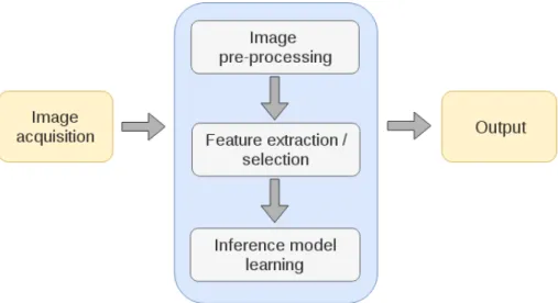
Figure 1.1: A typical image-based CAD system pipeline.

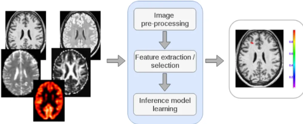
Image-based CAD systems are designed to apply an automated model on the given in-put images, so as to produce an outin-put corresponding to the problem [van Ginneken et al., 2011]. As illustrated on fig. 1.1, a typical CAD system entails the following steps - image pre-processing, feature extraction/selection and inference model learning (typically using a machine learning algorithm). Fig. 1.2 illustrates a CAD system taking at input mul-timodality neuroimaging data and outputting a probabilistic map highlighting suspicious areas found by the system.

(24)

1.1. GENERAL CAD DESCRIPTION

Figure 1.2: A CAD system for neuroimaging. Input: multimodality neuroimaging data. Output: Probabilistic map highlighting suspicious areas detected by the CAD system.

Input-output granularity

In a CAD system, the input may correspond to an image voxel, an image patch, a region of interest (ROI) or the entire image. The first three cases have the advantage of a smaller data size in comparison to the full image approach. The output of a CAD system may be at level, ROI-level or image (subject) level. For voxel-level CAD systems, each voxel is assigned a value produced by the system, eventually constituting an output map. For subject-level CAD systems, the output corresponds to the given image as a whole.

Image pre-processing

Typically, the CAD input images are first processed in order to enhance their quality. Common pre-processing steps include reduction of artifacts, noise reduction, image normalization, etc.

Feature extraction/selection

This step associates the input images with a set of characteristics (features) measured on the image following some definition/formula, relevant to the task at hand. For example, clinical knowledge on the pathology in question may be translated to a set of mathematical formulae and produce a set of descriptors of the pathology. Feature selection can further be performed in order to select the most relevant descriptors and discard the redundant ones. The features may also be learnt in an automatic data-driven fashion. In many recent applications this step is incorporated into deep architectures tailored to the task.

Inference model learning

In this step an inference model is built either based on the explicit descriptors ac-quired in the previous step or on the raw data. The choice of the model depends on the particularity of the task: it can be supervised (labels are available), unsupervised (labels are not available) and semi-supervised (labels are somewhat available). Below we present some more details on these steps.

Z. Alaverdyan 9

(25)

1.1.1 Input-output granularity

The granularity of the system depends on the desired outcome and the clinical need. CAD systems may be broadly categorized in two types. CADe systems seek to identify abnormal regions of a given image with respect to the pathology of interest. CADx systems aim at characterizing the pathology, its type/category, stage and severity [Petrick et al., 2013]. Image voxels, patches, ROIs and entire images may serve as input to CADs. The main categories of CADs with respect to the output granularity are:

Subject-level CADs

In this case the desired outcome of the CAD is usually to classify an image of a given subject into some category. Commonly such CADs perform binary classification by discriminating healthy versus pathological cases. The output may be expressed as a probability or a label. While it is possible to locate approximately the abnormal zone resulting in the binary output, its detection is not the main objective and usually is not performed. Some CADs are used to classify a given image into one of the categories of the pathology.

ROI-level CADs

In this case the model is based on a part of the input image corresponding to the region of interest (ROI), delineated by a radiologist; the remaining part is either irrelevant to the task at hand or is not significant and, hence, is not considered by the CAD system. Especially when the feature extraction step is applied explicitly, reducing the focus to a ROI instead of the full image allows acquiring relevant features over the ROI and reduce the dimensionality of the input data. The output of ROI-level CADs is a ROI-level score or label.

Voxel-level CADs

Some very popular CADs are designed to discriminate each voxel and produce either a probabilistic score map or a binary/n-ary map where each voxel is assigned a probability of being pathological or a binary/n-ary label representing the category it has been classified into.

1.1.2 Feature extraction and selection

An explicit extraction of features from the raw data has been a common choice for a very long time. In some medical applications there may be an accumulated clinical knowledge on the characteristics of the pathology of interest which can be translated into features by using appropriate formulae (table3.1lists such characteristics and their corresponding features for epilepsy). This certainly helps the discrimination of the pathology. However, in many contexts such knowledge is either not available or is insufficient and, hence, other

(26)

methods are exploited to extract features. For instance, one common approach is to extract generic image descriptors including

1. textural features describing textural patterns, frequently represented by statistical measures computed over a neighborhood (mean, standard deviation, etc) or derived from the grey-level co-occurrence matrix as described in [Haralick et al., 1973] (con-trast, entropy, energy, etc). The latter matrix models the joint probability density of the occurrence of grey levels for two pixels with a spatial relationship defined by the chosen relative direction and the distance between the two pixels.

2. local descriptors (filters) to detect edges and shapes such as Gabor filters [Manjunath and Ma, 1996] that can be viewed as a sinusoidal plane of particular frequency and orientation, modulated by a Gaussian envelope.

3. robust image descriptors such as HOG [Dalal and Triggs, 2005], SIFT [Lowe, 1999] and SURF [Bay et al., 2006]. SIFT (scale invariant feature transform) combines a scale invariant region (key point) detector and a descriptor represented by the histogram of the gradient distribution in the detected regions.

By varying the parameters of such image descriptors (such as the relative direction and the voxel distance in Haralick features) a very large number of features can be obtained. Typically, such a choice of features is accompanied by a feature selection strategy which consists in keeping only the most relevant feature subset and discard the rest. Since it is computationally exhaustive to evaluate all possible subsets and keep the most discrim-inative one, other practical strategies have been proposed for feature selection. As such, forward-stepwise (backward-stepwise) feature selection consists in greedily adding (elimi-nating) the most (least) informative feature starting from the empty (full) set of features. The informativeness of the candidate features in each step is measured by some quantity, for instance Akaike Information Criterion (AIC) [Akaike, 1974]. Recursive feature elimina-tion [Guyon et al., 2002] is another feature selection method that starts by fitting a model, that assigns weights to features (such as the coefficients of a linear model), to the entire feature set and later eliminates the features with the smallest weights. The procedure is performed recursively on the current feature subset. Feature selection may improve the performance of the system by eliminating irrelevant or redundant features and enhance the interpretability of the system, especially when the number of features is greater than the number of examples [Guyon and Elisseeff, 2003].

Features obtained in such way are referred to as handcrafted /manual features. The major disadvantage of such descriptors is their limited capacity in modeling complex phenomena as they are constrained with the kind of transformation they are designed to perform. Moreover, these features are not data-dependent and, hence, do not leverage the particular patterns that may be present in the data. Mainly for this reason there has been a major

Z. Alaverdyan 11

(27)

shift over the last years from handcrafted features to data-driven features automatically learnt from the data [Litjens et al., 2017]. Neural networks are one way of accomplishing data-driven feature learning (more details will follow in chapter2).

1.1.3 Inference model learning

The vast majority of the state-of-the-art CAD systems for various applications employ machine learning algorithms in order to build automated models that perform the task at hand. Such models take into account the nature of the application, the available data and the particularity of the problem.

A typical learning problem has the following setup. Given a data set of n observations X = {xi|i = 1, ..., n} generated by a fixed but unknown distribution P (x), a machine

learning algorithm seeks to model a function f (x) that, depending on the nature of the algorithm, outputs a relevant value for a (previously unseen) observation. Machine learn-ing algorithms can be broadly categorized into two major groups - supervised learnlearn-ing methods and unsupervised learning methods.

In supervised learning, a set of output values Y = {yi|i = 1, ..., n}, associated with the

examples in X, following a fixed but unknown conditional distribution P (y|x), is available. The learning algorithm seeks to find a function f (x; θ), characterized by a set of parame-ters θ, that approximates Y as accurately as possible. When Y is composed of continuous numerical values, the problem is referred to as regression problem; when Y takes values from a finite set of discrete values (labels), the problem is called classif ication problem. The classification problems may further be divided into binary (K = 2) and multiclass (K > 2) classification.

In unsupervised learning, no labels are associated with the observations and an unsuper-vised learning algorithm seeks to discover the properties of the data set, usually based on the distribution P (x).

Below we present the most common supervised and unsupervised methods used in mod-ern CAD systems. Since most CAD systems are designed to solve classification tasks, we will not detail on the regression methods. A particular case of the classification problems relates to the contexts where all observations have the same label (one-class classification) and will be presented separately due to its specificity.

I Supervised learning

As stated above, supervised learning methods seek to model a function f (x; θ), character-ized by a set of parameters θ, that predicts Y as accurately as possible. In order to pick the best function f from a set of candidate functions F parameterized with θ, a loss func-tion L(f (x; θ), y) quantifying the discrepancy between the predicted value and the actual output is necessary. Finally, the function f (x; θ∗) corresponding to the optimal parameter

(28)

set θ∗is the one that minimizes the expectation of the loss function, referred to as true error

θ∗ = argmin θ R(θ) where R(θ) is R(θ) = E [L(f (x, θ), y)] = Z L(f (x, θ), y)dP (x, y)

As P (x, y) is unknown, R(θ) is replaced by the empirical error Remp(θ) estimated on the

given training data set X

Remp(θ) = 1 n n X i=1 L(f (xi, θ), yi)

Typically, the evaluation of a model is performed on a set of observations not seen by the algorithm during training (referred to as test set ) but generated by the same distribution as the training set. The algorithm is expected to perform well on the unseen data. In this case the model will be said to generalize well; otherwise it overfits the training set. The generalization ability of a model depends largely on the assumptions and choices made during the training. In particular,

1. The success of the model depends on how representative the training set is for the data distribution of the given task. If the training data set represents adequately the distribution generating it, it will be reasonable to expect the algorithm to perform well on previously unseen data. When the training data set is not a representative subset of all possible observations, the model trained on it will learn to approximate the given observations, only to perform poorly on observations different from the training set i.e. it overfits.

2. Different families of candidate functions may be selected when designing an algo-rithm. Each family provides functions with different properties. The choice of the candidate functions should therefore be in line with the known properties of the data set at hand.

3. Most families of functions come with hyper-parameters that need to be tuned to achieve the best performance. The hyperparameters are usually chosen among a wide range of values by optimizing the performance on a set of observations, different from both training and test sets, called validation set. Improper hyperparameter values may lead to overfitting.

It is common to constraint the considered family of functions by adding a regularization term constraining its structure in order to improve the generalization properties of the learning method. In this case, the empirical error is enhanced with an additional term:

Remp(θ) = 1 n n X i=1 L(f (xi, θ), yi) + γ · Ω(f, θ) (1.1) Z. Alaverdyan 13

(29)

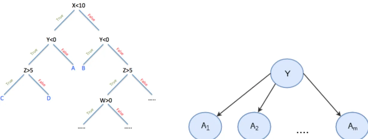
Figure 1.3: (a) A decision tree for a data set of 4 features - X, Y, Z and W, and 4 classes - A, B, C and D. (b) An illustration of Naive Bayes DAG for the variables A1, ..., Am and

class variable Y .

Below we briefly present some common supervised classification methods. A more complete description of the methods is included in the review by [Kotsiantis et al., 2007].

• Decision trees

Decision trees [Murthy, 1998] are structures that classify instances by consecutively check-ing the value of each of their features. Each node in a decision tree corresponds to a feature and each outgoing branch represents a possible value the feature can take on. The leaves of the tree correspond to the classes an instance is supposed to be categorized into. An optimal decision tree would contain the most discriminative feature at its root and each consecutive node would be assigned the most discriminative feature given its parent nodes. Building an optimal decision tree is a NP-complete problem and therefore heuristics are used in practice. An important component of building a decision tree is the choice of the metric with respect to which the features are chosen at each node. The most common of such metrics are information gain [Kent, 1983] and gini index [Breiman, 2017]. In order to prevent overfitting in decision trees, a strategy called pruning may be used that consists in disregarding the bottommost sub-trees in the built decision tree. Another practice is to employ an ensemble learning method, random forest, composed of multiple decision trees, that outputs a decision based on the outputs of all the trees in the forest e.g. with the majority voting. An example of a decision tree is shown on fig. 1.3a.

• Bayesian networks

A Bayesian network [Jensen, 1996] is a graphical model describing the relationships be-tween the features/variables. The structure of a Bayesian network is given by a directed acyclic graph (DAG) where each node corresponds to a variable in the given data set. The (conditional) dependence/independence relationships between the variables are modeled with particular structures in the graph. The second component of a Bayesian network

(30)

is the conditional probability tables quantifying the relationships between each node and its parents. Learning a Bayesian network assumes learning the structure of the DAG and estimating the conditional probabilities (parameters). Learning the exact DAG structure requires an exhaustive search among a number of candidates, exponential to the number of variables. Methods based on greedy search have been proposed for practical uses [ Chick-ering, 2002,Tsamardinos et al., 2006]. When the DAG structure is known (usually given by the experts), only the parameter estimation is necessary. The latter is usually achieved by maximizing the joint probability of the network. Naive Bayes is the simplest Bayesian network with a very primitive DAG composed of a single root (the class variable to predict) and its child nodes, conditionally independent of each other given the class variable, as illustrated on fig. 1.3b. This simple structure makes very strong assumptions on the rela-tionships between the variables which is almost never true; however, it results in a simple expression of the joint probability and the estimation of the parameters becomes straight-forward with Maximum Likelihood Estimation. The joint probability in Naive Bayes is given by p(Y, A1, A2, ..., Am) = p(Y ) m Y i=1 p(Ai|Y )

where Y is the class variable, Ai is the i-th variable. The decision ˆy for an example x is

then given by ˆ y = argmax k∈{1,..,K} p(Y = k) m Y i=1 p(xi|Y = k) • Instance-based methods

Instance-based methods are a category of approaches that delay the model inference to the point of classification of the test data. This means that the heavy computation phase is performed not during the training (like for other approaches above) but over the test time. k-Nearest Neighbour algorithm [Cover and Hart, 1967] is the most popular method of this category. The main assumption is that data points located in close vicinity have common properties, such as belonging to the same class to predict. Therefore, the class of a test point can be determined by the known classes of the points surrounding it (typically with a majority voting). It is necessary to provide the number of points to consult for the decision - the parameter k of the model (hence, the name). It is also necessary to choose a proper distance metric in order to determine the k-nearest neighborhood of an observation (Euclidean instance being a common choice). The fact that to classify an instance it is necessary to evaluate its distance to all the other points (which should be stored for testing) makes the method less practical for large-scale problems.

Z. Alaverdyan 15

(31)

Figure 1.4: An illustration of SVM. The examples of the two classes are marked with black/white circles.

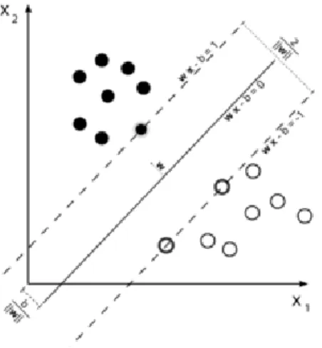
• Support Vector Machines

Support Vector Machines (SVM) are a very common supervised learning method intro-duced in [Vapnik, 1995]. SVMs seek to find a hyperplane separating the points of the two classes (yi ∈ {1, −1}) in a way that maximizes the distance between the hyperplane and

the closest point at either side of it (the distance is referred to as margin), as shown on fig. 1.4. The decision for an unseen example depends only on the linear combination of the points lying on the margin, called support vectors. To avoid the problem of misclassified training examples present in the data which do not allow the algorithm to find an optimal hyperplane, a soft margin formulation allows the misclassification of some examples, at a cost added to the term maximizing the margin. In this case using SVMs boils down to minimizing the following cost

argmin w,b 1 n n X i=1 max(0, 1 − y_i(w · xi− b)) + λ||w||2

where xiis the i-th example, yiis its corresponding class label, n is the number of examples,

w and b define the hyperplane and λ is the tradeoff coefficient controlling the number of misclassified examples. The first term is the hinge loss and one can recognize the explicit form of the empirical error R_emp given in1.1.

As the points may not be linearly separable in the original feature space, it is common to use the so called kernel trick to project the points to a higher dimensional space where the points are better separated. To use the kernel trick it is necessary to select the kernel function, the most common being radial basis function (RBF) kernel and polynomial kernel, each coming with hyperparameters to tune (more details on the kernel trick will be given in section 5.1.3). The SVM optimization problem eventually reaches a global minimum which has made it a very popular method. Some strategies have been proposed to extend the binary SVM for a multiclass classification, for example, through building SVMs for each class versus all the rest combined.

(32)

(a) A neuron, the computational unit in neural networks. w and b are the weights and bias associated with it, a is the input and g is a (usually non-linear) activation function.

(b) A simple artificial neural network with 2 hidden layers.

Figure 1.5: Artificial neural networks.

• Artificial neural networks

Artificial neural networks (ANN) are a category of methods vaguely resembling the neural network of animal brains. ANNs [Rosenblatt, 1958,LeCun et al., 1989] consist of compu-tational units called neurons that together form a layer. A neuron is shown on fig. 1.5a. Layers may be stacked to form more complex structures as shown on fig. 1.5b. The neurons of one layer are connected to the neurons of the previous layer. The last layer in a typical neural network corresponds to the classification (less frequently, regression) task at hand. The structure particular to ANNs allows learning representations describing the input at different levels. So, the first layers usually capture more primitive patterns present in the input while the topmost layers model abstract representations. The main advantage of ANNs is that there is no need to gather relevant feature vectors to perform training; the relevant features are being learnt while training the network for the task at hand. Formally speaking, the connections between the units in the network are modeled with a (usually) non-linear function on top of a linear transformation of the incoming neurons. ANNs are the core of the so-called deep learning methods which will be presented in more details in the next chapters.

I Unsupervised learning

The setup for unsupervised machine learning problems is similar to the one for super-vised methods, the difference being that there is no output vector Y associated with the training examples. Unsupervised methods aim at learning some hidden structure in the data set that can be useful to discover and describe the tendencies and patterns for the given task and the data. It is more difficult to evaluate the quality of an unsupervised method, unlike in the supervised setting, where the true output is given and comparing it to the predictions is straightforward. The most common application of unsupervised learning is clustering.

Z. Alaverdyan 17

(33)

Clustering

Clustering or cluster analysis algorithms seek to partition the given data points into cohe-sive groups of points similar or close to each other with respect to some measure, so called clusters. Clustering, therefore, may reveal interesting information on the structure of the data set. The most common clustering methods are listed below. A detailed review of clustering methods has been done in [Jain et al., 1999] and [Xu and C. Wunsch II, 2005].

1. Hierarchical clustering

Hierarchical clustering methods aim at partitioning the data points based on their distance by building a dendrogram, a hierarchy of levels, each level yielding a set of clusters. The advantage of such methods is that cutting a dendrogram at different levels allows obtaining a certain number of clusters, without retraining the model. The construction of a dendrogram can proceed in either agglomerative or divisive approach. The former starts by considering each data point as a cluster and further recursively merges the current clusters by combining the closest pairs. The divisive approach starts with a single cluster containing all data points and recursively splits the current clusters into smaller ones by separating the farthest points. In either case a measure of distance between entities is necessary. Most common distance choices are implemented in single linkage clustering, complete linkage clustering, average linkage clustering and Ward’s clustering [Ward Jr, 1963]. More hierarchical clustering methods are discussed in [Murtagh and Contreras, 2011].

2. k-means clustering

k-means clustering [MacQueen et al., 1967] seeks to partition the data points into a set S of k clusters by minimizing the sum of squared error (SSE) criterion quantifying the within-cluster variance (the sum of the distances of the points to their cluster center) given by argmin S k X i=1 X x∈Si ||x − c_i||2

where c_i is the centroid of cluster S_i. It proceeds by randomly selecting k points as cluster centroids and further alternates between two steps - 1. assigning each data point to the cluster with the closest centroid and 2. updating the current cluster centers with the centroids of the newly found clusters. k-means is sensitive towards the initialization of the method, though multiple initialization approaches have been proposed as discussed in [Celebi et al., 2013]. The choice of the optimal cluster number k can be made by monitoring the changes in the SSE as the number k is varied through some range and pick the value resulting in minimal SSE or 1 standard deviation away from it (elbow method).

(34)

3. Mixture model clustering

Mixture model based clustering assumes the cluster to be a random variable z of K possible values whose prior distribution p(z) and the conditional probability function of an example x given the cluster variable p(x|z) are known. Gaussian mixture models (GMM) is the most common configuration of such approaches where p(z) is categorical/multinoulli distribution i.e. p(z = k) = π_k,PK

k=1πk = 1 and p(x|z)

is a Gaussian distribution with a mean vector µ_k and covariance matrix Σ_k i.e. p(x|z = k) ∼ N (µk, Σk). The GMM training consists in estimating the parameters

of those distributions which is usually done with maximum likelihood estimation, yielding the parameters that maximize the joint probability over the entire data set, given by L(θ1, ..., θK; π1, ..., πK|X) = n Y i=1 K X k=1 πkN (xi; θk)

where θ_k= (µk, Σk). The most commonly exploited method to do so is the

Expecta-tion - MaximizaExpecta-tion (EM) algorithm [McLachlan and Krishnan, 2007]. The algorithm proceeds in repeating two alternating steps - 1. e-step: compute the expectation of the complete data log-likelihood, 2. m-step: select new parameter estimates max-imizing the previously computed function (k-means is a particular case of the EM algorithm). The posterior probability p(z|x) of a cluster given an observation is then calculated with the Bayes’ theorem using the estimated parameters.

For most clustering methods, it is required to decide upon the desired number of clusters K. The choice may be intuitive for some small-scale and relatively simple tasks but in the vast majority of real life problems, the choice of K is not trivial: small Ks may give little information on the structure of the data while greater values may reduce the interpretabil-ity. Several approaches exist to select an optimal K. In some cases a simple 2-dimensional visualization of the data points can give an idea of the order of K. For GMM, the num-ber of clusters can be chosen among a range of values as the one minimizing the Akaike’s information criterion (AIC) [Akaike, 1974] or maximizing the Bayesian inference criterion (BIC) [Schwarz et al., 1978]. The Gap statistic [Tibshirani et al., 2001], that compares the total within-cluster sum of squares for different values of K with their expected values under a null reference data distribution, can also be used, especially for k-means clustering.

I Outlier detection

One-class classification problems are a particular case of classification problems where the training set contains examples of only one class and the aim is to later identify the repre-sentatives of that class. An important application of one-class classification problems is the so called outlier detection. Outlier detection methods, also known as anomaly detection, novelty detection, seek to distinguish outliers from the normal examples constituting the given data set. All the examples of the given training data set are normal/positive and

Z. Alaverdyan 19

(35)

hence have the same label; the label however is not informative and does not appear any-where in the problem formulation, which is why outlier detection problems are usually seen as unsupervised problems. The definition of an outlier may vary across different domain applications and data sets. Essentially, outliers are examples that do not quite fit to the characteristics of the normal/inlier observations. More precise definitions may apply. So, [Hawkins, 1980] defines an outlier as an observation that deviates so much from other ob-servations as to arouse suspicion that it was generated by a different mechanism. [Johnson and Wichern, 1992] defines an outlier as an observation in a data set which appears to be inconsistent with the remainder of that set of data. A more thorough overview is presented in [Ben-Gal, 2005].

Over the recent years the topic of outlier detection has been studied extensively in different application domains and many algorithms have been proposed for outlier detection depend-ing on the nature of the data and the type of anomalies [Hodge and Austin, 2004,Chandola et al., 2009, Pimentel et al., 2014, Kiran et al., 2018]. Outlier detection methods have been applied in various domains and applications, including credit card fraud detection [Aleskerov et al., 1997], mobile phone fraud detection [Barson et al., 1996], network intru-sion [Lazarevic et al., 2003], fault identification [Diaz and Hollmén, 2002], etc. We identify 5 major categories of the existing outlier detection methods: (1) probabilistic, (2) distance-based, (3) reconstruction-distance-based, (4) domain-based and (5) information-theoretic. Below we present a brief summary of the assumptions and main characteristics of these meth-ods. More comprehensive reviews have been conducted in [Pimentel et al., 2014,Chandola et al., 2009].

1. Probabilistic methods

Probabilistic outlier detection methods aim at estimating the underlying probability density function generating the data and declaring outliers as data points largely deviating from the estimated density function. The main assumption of such meth-ods is that outliers correspond to low density areas whereas inliers are concentrated in the high density areas of the underlying distribution. Two major categories of probabilistic methods exist: parametric and non-parametric.

Parametric methods assume that the data has been generated by a parametric distri-bution with a parameter set Θ; Θ is estimated using the available data. Naively, the inverse of the probability function for a test point can be interpreted as a measure of its anomalousness. Other approaches are based on statistical hypothesis tests that consider the null hypothesis as the event that a given point has been drawn from the estimated distribution. When the null hypothesis is rejected, the point is consid-ered an outlier. For example, Grubb’s test [Grubbs, 1969] assumes the training set was generated by a Gaussian distribution and treats the points whose distance from the estimated mean is larger than a certain threshold as outliers. It was designed

(36)

for univariate analysis; its alternative versions were proposed in [Laurikkala et al., 2000,Aggarwal and Yu, 2001]. A more sophisticated approach chooses to model the underlying data distribution as a mixture of parametric distributions. For example, Gaussian Mixture Models (GMM) are a very popular method based on modeling a mixture of Gaussians and declaring a test point an outlier when it does not seem to be generated by any of them. The most common technique to estimate the parameters for this approach is maximum likelihood estimation, in particular, the EM algorithm. The successful application of this category of methods depends on how well the basic assumptions on the underlying distribution correspond to the data at hand and how much data is available to approximate well the distribution in question.

Non-parametric methods do not assume any a priori form for the underlying density function; it is determined from the training set. One simple non-parametric approach is the histogram-based method that "learns" the shape of the density function by constructing a histogram. It is done by defining bins and counting the number of data points falling into each of them for a particular feature. Once the histogram is built, a test point is considered an outlier if it is not included in any of the bins. The key point here is to choose the bin size. The main drawback is that the histograms are built for each individual feature; discriminating outliers by taking into account the (possibly) complex interactions between the features may not be achieved. Kernel density estimator, also known as Parzen window method [Parzen, 1962], is another common method of density estimation. It places a Gaussian distribution centered at each of the training examples and computes their linear combination. The only free parameter of this technique is the kernel width which controls the smoothness of the learnt distribution. The outliers are then detected as the points located in the low-density areas of the estimated distribution.

2. Distance-based methods

Distance-based outlier detection methods adopt the assumption that outliers are rather isolated data points and, therefore, their distance to their neighbors should be indicative of their anomalousness. k-nearest neighbor [Altman, 1992] is one of the approaches that considers a data point an outlier if its distance to its k-th neighbor is larger than a chosen threshold. A different category of methods consider the local density in the neighborhood of a point as an indicator of anomalousness. For instance, [Breunig et al., 2000] proposed a metric called Local Outlier Factor (LOF) defined as the ratio of the average density of the areas around the k nearest neighbors of a given point and the local density of the area around the point itself. In the LOF method, the local density, more precisely, the local reachability density, of a point is defined as the inverse of the average reachability distance of the point from its neighbors. Another approach called Local Outlier Probabilities (LoOP) combines the

Z. Alaverdyan 21

(37)

main idea behind LOF with a probabilistic component to model the anomalousness of an example [Kriegel et al., 2009]. Unlike the nearest neighbor based methods that make assumptions on the distance of a given point from its neighbors, cluster-based outlier detection methods make assumptions about the distance of the point to its closest cluster center. Basically, such an approach involves clustering the training data using any clustering method (k-means, for example) and declare outliers based on their distance to the found clusters. This method would not suit to the cases where outliers themselves are numerous and close enough to form a cluster of their own.

3. Reconstruction-based methods

Reconstruction-based outlier detection methods assume a model able to reconstruct a given input after having it transformed to some intermediate representation. The deviation between the reconstruction and the original input is then considered in-dicative for the detection of outliers. Two major categories of such methods are subspace-based and neural network based algorithms. Principal Component Analy-sis (PCA) is a popular subspace-based method [Jolliffe, 2011] that seeks to project the original observations of correlated variables to a space defined by uncorrelated variables (principal components) that maximize the variance of the data. It has been widely used as a dimensionality reduction technique (convenient as the method seeks to project the original data points to a space where the desired amount of the infor-mation can be preserved by keeping a certain number of principal components). The transformation applied to the original input may be interpreted as encoding and may be used to obtain a reconstruction of the input: the deviation of the reconstruction from the input can be used to indicate outliers. Kernel PCA [Schölkopf et al., 1997] extends the original formulation by first performing a mapping through a non-linear kernel into a higher-dimensional space and then applying the PCA. PCA-based out-lier detection was applied in [Huang et al., 2007,Brauckhoff et al., 2009,Choi et al., 2005]. Neural-network based anomaly detection methods will be reviewed in chapter 6.

4. Domain-based methods

Domain-based methods, unlike those that try to estimate the density of the given normal data points, seek to find their boundary. In this case the decision on the anomalousness of a given point depends on which side of the boundary the point is located. One class SVM (oc-SVM) [Schölkopf et al., 2001], a particular case of SVMs, is one of the most common methods of the category. It seeks to find a hyperplane with maximum margin separating the normal points from the origin. The kernel trick is usually applied and the separation is performed in a higher-dimensional space.

(38)

1.2. PERFORMANCE EVALUATION OF CAD SYSTEMS

Support Vector Data Description (SVDD) method [Tax and Duin, 2004] is formulated similarly to the oc-SVM method and aims at finding the hypersphere with minimum volume containing the normal points. A point laying outside of it is considered an outlier. The oc-SVM algorithm will be described in details in section5.1.3.

5. Information-theoretic methods

Information-theoretic methods are based on the idea of quantifying the information content of a data set as measured with entropy, conditional entropy, relative con-ditional entropy, information gain, information cost or other similar measures. The main assumption of these methods is that the presence of outliers changes dramat-ically the information content of a data set. Therefore, removing the outliers will have a significant impact on the measure of choice (e.g. entropy). Information theory-based methods seek to identify outliers as a subset of data points whose removal from the data set results in the largest change of the chosen measure as compared to the removal of the rest of the data points. [He et al., 2006] proposed a greedy algorithm (Local Search Algorithm) that iteratively labels the point with the largest entropy decrease among the points currently labeled as normal, as outlier, until the number of outliers reaches k, a preselected value. Choosing the value for the parameter k may not be intuitive in many applications and is a disadvantage of such an approach.

1.2 Performance evaluation of CAD systems

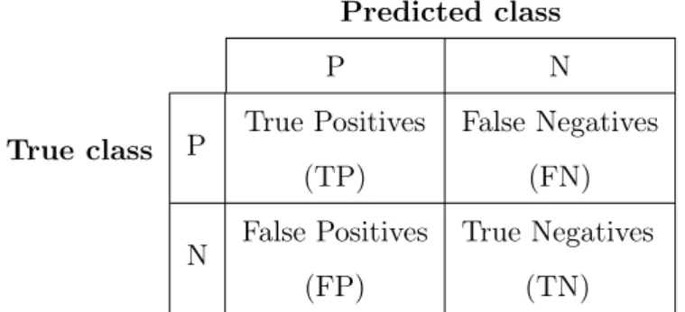
One crucial step of any CAD system is the performance evaluation. Evaluating a CAD system means assessing its generalization ability i.e. the capacity to perform the task of interest on previously unseen data. This amounts to estimating the expected prediction error (test or generalization error) at some new point. While annotated data may or may not be used during the model training phase, a typical CAD system evaluation involves comparing the output of the system to a reference. We will therefore focus on the evalua-tion protocol where the reference or ground-truth annotaevalua-tions are given for the evaluaevalua-tion. Formally, for a given training data set D = {(x_i, ti)} for i = 1, .., N , a trained model

pre-dicts an output y via a function f i.e. y = f (x). Assuming the optimal prediction is given by y∗ and L(t, y) is a loss measuring the discrepancy between t and y, the expected predic-tion error can be shown to have the following decomposipredic-tion for some learning algorithms [Domingos, 2000]

E[L(t, y)] = c1E[L(t, y∗)] + L(y∗, ym) + c2E[L(ym, y)]

where ym is some central tendency of the learnt model. The test error decomposition was first derived for regression, with L being the squared loss and c1= c2= 1 (full derivation in

[Hastie et al., 2009]). For a binary classification task, when L is the 0-1 loss, the expression above holds for certain values of c₁ and c₂. A closed-form expression exists in particular

Z. Alaverdyan 23

(39)

for k-nearest neighbor algorithm. The main objective of the decomposition above is to separate the three terms:

1. the first term is the irreducible error, independent of the learning algorithm and hence beyond our control

2. the second term is the bias of the learning algorithm, the difference of its predictions and the optimal predictions. The bias is 0 for a model always making optimal predictions

3. the third term is the variance of the learning algorithm quantifying the differences around the central tendency. A high difference between the average predictions on the training and test sets is indicative of high variance.

Good learning algorithms therefore are characterized with low bias and low variance. Find-ing the bias-variance tradeoff is an important aspect of selectFind-ing a model.

In the clinical settings, estimating the generalization error usually amounts to testing the CAD system on a new set of patients, not used for the training of the CAD system. The first aspect to consider is therefore a strategy to split the data into sets that would be used for training and later for evaluation. Eventually, an appropriate metric should be chosen to quantify the performance on the unseen data set. Below we discuss these two aspects in details.

1.2.1 Data splitting strategies

An essential part of building an automated system is to decide upon the training set, validation set and test set. The training set, as the name suggests, is composed of the observations which are used for the training. The validation set comprises the observa-tions not used for training but essential for the so-called model selection. Model selection consists in retaining a configuration, among a set of possibilities, that gives an acceptable performance on the validation set when trained on the training set. Frequently model selection boils down to selecting hyperparameters for an algorithm. Moreover, evaluating the system on the validation set creates a feedback that can be used to improve the current settings. Once the model is chosen and trained, it can be evaluated on a previously unused test set. The evaluation should be final and should not be used to modify the model after-wards. There exist several strategies of splitting the given data set into training, validation and test sets, depending on the availability of the data. When the overall data set contains a substantial number of observations, the most straightforward approach is a basic split into three distinct subsets, the training set typically being the largest. In many problems, especially in the medical domain and therefore in CAD development, the available data sets are scarce in the number of examples. For such cases, alternative strategies have been developed.