HAL Id: tel-01407352
https://tel.archives-ouvertes.fr/tel-01407352
Submitted on 2 Dec 2016
HAL is a multi-disciplinary open access archive for the deposit and dissemination of sci-entific research documents, whether they are pub-lished or not. The documents may come from teaching and research institutions in France or abroad, or from public or private research centers.
L’archive ouverte pluridisciplinaire HAL, est destinée au dépôt et à la diffusion de documents scientifiques de niveau recherche, publiés ou non, émanant des établissements d’enseignement et de recherche français ou étrangers, des laboratoires publics ou privés.
OH reactivity measurements in the Mediterranean
region
Nora Zannoni
To cite this version:
Nora Zannoni. OH reactivity measurements in the Mediterranean region. Analytical chemistry. Uni-versité Paris Saclay (COmUE), 2015. English. �NNT : 2015SACLS163�. �tel-01407352�
NNT : 2015SACLS163
T
HESE DE DOCTORAT
DE
L’U
NIVERSITE
P
ARIS
-S
ACLAY
PREPAREE A
“U
NIVERSITE
P
ARIS
-S
UD
”
E
COLED
OCTORALE N° 579
Sciences mécaniques et énergétiques, matériaux, géosciences
Spécialité de doctorat : Chimie atmosphérique
Par
Nora Zannoni
Titre de la thèse
OH reactivity measurements
in the Mediterranean region
Thèse présentée et soutenue à Gif sur Yvette, le 30/11/2015: Composition du Jury :
Prof. Dr. Laurent Salmon Université Paris-Sud Président
Dr. Coralie Schoemaecker Université Lille Rapporteur
Dr. Silvano Fares CRA-RPS Rapporteur
Dr. Matthias Beekmann LISA Examinateur
Prof. Dr. Nadine Locoge Mines Douai Examinatrice
Dr. Valerie Gros LSCE Directeur de thèse
OH reactivity measurements in the
Mediterranean region
A dissertation submitted to
Universit´e Paris-Saclay
for the degree of
Doctor of Chemistry
presented by
NORA ZANNONI
Laboratoire des Sciences du Climat et de l’Environnement
UMR 8212 CEA/CNRS/UVSQ
supervisor: Dr. Valerie Gros co-supervisor: Dr. Bernard Bonsang
reviewers: Dr. Nadine Locoge, Dr. Matthias Beekmann
examiners: Dr. Coralie Schoemaecker, Dr. Silvano Fares, Dr. Laurent Salmon
Contents
Abstract xv
R´esum´e xvii
1 Introduction to total OH reactivity 1
1.1 Theoretical background on tropospheric chemical processes and reactive
constituents . . . 1
1.1.1 Atmospheric relevance of reactive gases . . . 2
1.1.2 The hydroxyl radical and other atmospheric oxidants . . . 3
1.1.3 Nitrogen Oxides . . . 5
1.1.4 Volatile Organic Compounds (VOCs) . . . 6
1.2 Total OH reactivity: a change in philosophy . . . 15
1.2.1 OH reactivity relevance . . . 16
1.2.2 Measuring the OH reactivity . . . 18
1.2.3 OH reactivity in the world . . . 20
1.2.4 The missing OH reactivity . . . 23
1.3 The Mediterranean basin . . . 24
1.3.1 General aspects . . . 24
1.3.2 Natural and anthropogenic local emissions . . . 25
1.3.3 A hotspot for climate change . . . 28
1.4 Thesis objectives . . . 30
2 Experimental 33
2.1 Proton Transfer Reaction-Mass Spectrometer (PTR-MS) . . . 33
2.1.1 Applications in atmospheric sciences . . . 33
2.1.2 Instrumental operation . . . 34
2.1.3 Compounds sensitivity and volume mixing ratio . . . 36
2.2 Comparative Reactivity Method for OH reactivity studies . . . 37
2.2.1 General principle . . . 37
2.2.2 Derivation of the basic equation for CRM . . . 38
2.2.3 The reactor . . . 39
2.2.4 The detector . . . 40
2.2.5 Method calibration . . . 41
2.2.6 Interferences . . . 42
2.2.7 Data processing . . . 44
2.2.8 Limit of detection and measurement uncertainties . . . 49
2.3 CRM-LSCE . . . 49
2.3.1 Optimization of the Comparative Reactivity Method at LSCE . . . 49
2.3.2 CRM-LSCE performance . . . 53
2.3.3 CRM-LSCE: field deployment . . . 56
3 Intercomparison of two comparative reactivity method instruments in the Mediterranean basin during summer 2013 61 3.1 Introduction . . . 62
3.2 Experimental . . . 65
3.2.1 The comparative reactivity method . . . 65
3.2.2 Data processing . . . 67
3.2.3 Comparative Reactivity Method set up . . . 70
3.2.4 Description of the field site and experiments . . . 74
3.3 Results and discussion . . . 75
3.3.1 C1 acquired with the conventional and scavenger approaches . . . . 76
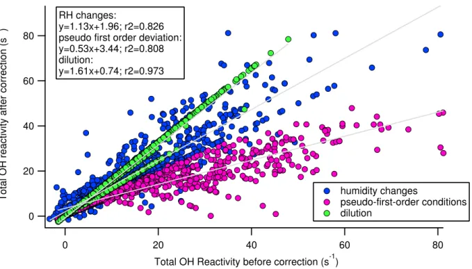
3.3.2 Assessment of the correction for humidity differences between C2
and C3 . . . 78
3.3.3 Assessment of the correction for the kinetics regime . . . 79
3.3.4 Correction for dilution . . . 81
3.3.5 Measurement uncertainty . . . 83
3.3.6 Intercomparison of OH reactivity results . . . 83
3.4 Summary and conclusions . . . 86
4 OH reactivity and concentrations of Biogenic Volatile Organic Com-pounds in a Mediterranean forest of downy oak trees 89 4.1 Introduction . . . 90
4.2 Methodology . . . 93
4.2.1 Description of the field site . . . 93
4.2.2 Ambient air sampling . . . 94
4.2.3 Comparative Reactivity Method and instrument performance . . . 95
4.2.4 Complementary measurements at the field site . . . 97
4.2.4.1 Proton Transfer Reaction-Mass Spectrometer . . . 97
4.2.4.2 Gas chromatography-flame ionization detector . . . 99
4.2.4.3 Formaldehyde analyzer . . . 100 4.2.4.4 NOx analyzer . . . 101 4.2.4.5 GC-MS offline analysis . . . 101 4.2.4.6 O3, CH4, CO . . . 101 4.2.4.7 Meteorological parameters . . . 101 4.3 Results . . . 102
4.3.1 Trace gases profiles and atmospheric regime . . . 102
4.3.2 Total OH reactivity . . . 105
4.3.3 Measured and calculated OH reactivity . . . 106
4.3.4 Nighttime missing reactivity . . . 109
4.3.5 OH reactivity at other biogenic sites . . . 112
4.4 Summary and conclusion . . . 114
5 Total OH reactivity at a receptor coastal site in the Mediterranean basin
during summer 2013 117
5.1 Introduction . . . 118
5.2 Field site . . . 119
5.3 Methods . . . 120
5.3.1 Comparative Reactivity Method . . . 120
5.3.2 Ancillary measurements at the field site . . . 123
5.3.2.1 Proton Transfer Reaction-Mass Spectrometry . . . 123
5.3.2.2 Online Chromatography . . . 125
5.3.2.3 Offline Chromatography . . . 126
5.3.2.4 Hantzsch method for the analysis of formaldehyde . . . 126
5.3.2.5 Chemiluminescence for the analysis of NOx . . . 127
5.3.2.6 Wavelength-scanned cavity ring down spectrometry (WS-CRDS) . . . 127
5.3.3 Box model for mixing ratios and OH reactivity evaluation . . . 128
5.4 Results . . . 130
5.4.1 Air masses regime . . . 130
5.4.2 Total measured OH reactivity . . . 131
5.4.3 Calculated OH reactivity and importance of biogenic VOCs at the measuring site . . . 132
5.4.3.1 Long-term variability . . . 132
5.4.3.2 Contributions from different classes of compounds . . . 133
5.4.3.3 Impact of biogenic VOCs . . . 135
5.4.4 Comparison between measured and calculated reactivity . . . 137
5.4.5 Clues on the missing OH reactivity: a mix of primary emission and secondary production . . . 138
5.4.5.1 Unmeasured terpenes . . . 138
5.4.5.2 estimated reactivity of the unmeasured terpenes . . . 139
5.4.5.3 unmeasured secondary products . . . 140
5.4.6 Modeled OH reactivity . . . 142
5.4.6.1 Model inputs . . . 142
5.4.6.2 Model results and sensitivity . . . 143
5.4.6.3 Contributions to the modelled OH reactivity . . . 145
5.5 Conclusions . . . 146
5.6 Acknowledgments . . . 147
6 Conclusion and future research 149
A Rate coefficients of reaction with OH for selected atmospheric
com-pounds 155
B Selected Poster Presentations 157
List of Tables 161
List of Figures 163
Bibliography 167
Preface
This thesis describes the work I have done during my PhD studies at Laboratoire des Sciences du Climat et de l’Environnement (LSCE) between November 2012 and October 2015.
The project concerns the technical optimization of the Comparative Reactivity Method (CRM) for measuring the total OH reactivity and field measurements of OH reactivity at targeted sites in the Mediterranean region.
The findings discussed in this thesis are the results of an experimental work conducted in the laboratory of LSCE for building and testing the technique of the CRM and of an experimental field work. The field work was performed during two main campaigns: ChArMEx (the Chemistry-Aerosol in a Mediterranean Experiment), during summer 2013 and CANOPEE (Biosphere-atmosphere exchange of organic compounds: impact of intra-canopy processes), during spring 2014. Field measurements were conducted for determin-ing the total loaddetermin-ing of reactants and our level of understanddetermin-ing of the reactive composition of the air masses influencing the sites.
The project is part of the European Marie Curie Innovative Training Network ”PIMMS” (Proton Ionization Molecular Mass Spectrometry) which aims at developing molecular mass spectrometry techniques in different field of sciences, including environmental, food and medical sciences. This thesis project was funded through PIMMS because of the use of proton ionization mass spectrometry for measuring the OH reactivity. The PIMMS network provided me and this project the tools and means to improve the quality of this work, including visits to IISER Mohali, India to discuss about the CRM with Dr. Vinayak Sinha; Ionicon, Austria, to develop my knowledge on proton transfer molecular mass spectrometry; Juelich, Germany to participate to a field campaign on aerosols formation at the atmospheric chamber SAPHIR.
This thesis consists of six chapters. The first chapter provides an introduction to the concept and importance of OH reactivity. It is composed by four sections, i.e., background to tropospheric processes and composition, OH reactivity, the Mediterranean basin, and
the thesis goal. The first section discusses in detail the main players in tropospheric reactions, i.e., the hydroxyl radical, nitrogen oxides and volatile organic compounds and reactions they undergo. The second section describes the originality of the concept of OH reactivity and the need of developing it. It provides an overview of the methods currently existing for measuring the OH reactivity and values of OH reactivity observed from ground-state field measurements at different point sources in the world. Finally it reports the main findings on the missing reactivity, which is now a topic of great interest in atmospheric sciences. The third section introduces the Mediterranean basin as a region of great interest for atmospheric chemistry studies. It explains the main sources of pollution and why measurements of reactivity are needed in this part of the world. Finally, the last section describes specifically the goal and research questions that this project addresses. The research questions are answered specifically in the chapters 3, 4 and 5.
The second chapter is divided into three sections. The first two sections provide the theoretical background of the two main methodologies applied in this project: Proton Transfer Reaction-Mass Spectrometry (PTR-MS) and the Comparative Reactivity Method (CRM). The section of the CRM describes in detail the updated theory of the method, and includes its concept, operational settings and data processing. The third section focuses on the progresses made during this PhD project in our laboratory. It includes technical improvements for increasing the sensitivity of the method and improvements to reduce the stated interferences. It gives an overview of the performance of our instrument, here referred as CRM-LSCE and the performance of our instrument during the two field campaigns whose results are described in the following chapters.
The third chapter presents the findings of an intercomparison exercise run between CRM-LSCE and the instrument built at Mines Douai, France (CRM-MD) published as Zannoni et al., (2015a) on Atmospheric Measurements and Techniques. It includes a detailed description on the way to assess the corrections of the raw data and the way to process them on ambient raw data of reactivity. It shows the results of the tests and ambient measurements of reactivity run during July 2013 on the field in Corsica, France. It shows how the different corrections impact the raw data for each instrument and how the final
processed data correlate well between them over the range of reactivity of 0-300 s−1. It
highlights the importance of conducting a detailed experimental characterization of each CRM instrument and of extending intercomparison practices to more instruments using different techniques.
The fourth chapter presents the results of a field campaign conducted in the forest of downy oaks of Observatoire de Haute Provence (OHP) where the concentration of volatile organic compounds and OH reactivity were simultaneously measured. The results are shown in
the form of the article, published on Atmospheric Chemistry and Physics Discussions as Zannoni et al., (2015b). Here, the total loading and distribution of reactants at two heights of the forest: inside the canopy (i.e. 2 m) and above the canopy (i.e. 10 m) are presented. Comparison between the measured and calculated reactivity reported no difference during daytime observations, while large gaps were observed during nighttime. Finally, the chapter gives a perspective on values of OH reactivity measured in different forests of the world. It shows that the Mediterranean forest of OHP emits large amounts of reactive species, only comparable to tropical forests.
The fifth chapter is a preliminary draft of an article I wrote describing the main findings obtained from the measurements of OH reactivity during the field campaign ChArMEX. This draft includes the work of other scientists from LSCE (France), the laboratory of Mines Douai (France), LamP, Clermont Ferrant (France), which are not specifically men-tioned as the draft was not distributed before this thesis submission. This chapter includes a description of the time series and diurnal profile of the OH reactivity measured during summer 2013 at the receptor field site of Ersa, Corsica, France. It includes a comparison between the measured reactivity and the one calculated from the species measured in the gas-phase. It provides some hypothesis on the discrepancy observed between these two parameters during one week of measurements. Finally, it provides the preliminary results of a chemical model used to determine the oxidation products of the biogenic compounds measured at the site and their contribution to the OH reactivity. The simulations were run by Dr. Sophie Szopa (LSCE) and aim at providing an idea of the type of information that can be obtained by combining the results from the measurements with a modelling approach.
Finally, chapter 6 is the outlook and conclusions of this PhD project, including some suggestions for further research.
Abstract
The hydroxyl radical, .OH, is the dominant oxidant in the atmosphere: it can initiate
most of the oxidation reactions involving volatile organic compounds and leading to the formation of ozone and aerosols; with adverse effects on the air quality and climate. There are many uncertainties associated to the total sink of the OH radical, because it is difficult to characterize all the reactive species responsible for its loss in the atmosphere. The total OH reactivity is defined as the total first order loss rate of OH due to the atmospheric reactive gases and represents the total sink of OH. This parameter directly provides the total loading of reactive gases in ambient air and indicates the frequency of the oxidation reactions involving OH and reactive molecules.
Measurements of OH reactivity have many utilities, among them, they can be compared to the OH reactivity calculated from simultaneous measurements of reactive gases and highlight whether all these gases are measured and known or not. Several studies using such approach have highlighted that a significant fraction of reactive gases is not measured and possibly unknown. Especially, larger fractions of missing reactivity have been reported in forests and in those environments characterized by larger loadings of secondary or higher generation oxidation products.
In this thesis, the Comparative Reactivity Method (CRM) for measuring the total OH reactivity is deployed in an intercomparison exercise and at two targeted sites in the Mediterranean basin.
I here report a detailed characterization of a comparative reactivity method instrument built in our institute (Laboratoire des Sciences du Climat et de l’Environnement) and explain the technical improvements conducted during my PhD project. The instrument was constructed and characterized to specifically measure the OH reactivity at two sites exposed to different field constraints. In addition, the instrument performance was com-pared to the one of another CRM instrument built in another laboratory (Mines Douai, France). The intercomparison exercise highlighted that our measurements were
repro-ducible in a range of reactivity between the instrument limit of detection and 300 s−1 and
that a precise characterization of each CRM is needed.
Ambient OH reactivity was measured at two sites: at a receptor site in Corsica (field campaign ChArMEx, summer 2013) and in a forest of downy oaks in Provence, in the south of France (field campaign Canopee, spring 2014).
Both field studies highlighted two main points : (i) the targeted sites in the Mediterranean basin are both exposed to large loadings of reactive molecules, (ii) a detailed characteriza-tion of the atmospheric composicharacteriza-tion, including the products formed by oxidacharacteriza-tion reaccharacteriza-tions, is still challenging. Deploying the OH reactivity tool at other field sites and in laboratory studies would be of great benefit to better understand atmospheric processes, especially focusing on plants emissions and chemical transformation. Investigating more field sites in the Mediterranean region is also recommended to have a greater picture on the loading of reactants in this area.
R´
esum´
e
Les radicaux hydroxyles (OH) sont les oxydants majeurs de notre atmosph`ere. Ils in-terviennent dans les processus d’oxydation de nombreux polluants atmosph´eriques, et notamment des composes organiques volatils (COV), et conduisent `a la formation d’ozone et d’a´erosols organiques ; ces derniers ayant des effets adverses sur la qualit´e de l’air et le climat. De nombreuses incertitudes existent quant `a l’estimation du puit total des radicaux OH, en raison de la difficult´e que repr´esente la caract´erisation exp´erimentale de l’ensemble des compos´es qui contribuent `a leur consommation dans l’atmosph`ere. En effet, les COV repr´esentent une famille de plusieurs centaines de mol´ecules, pr´esents dans l’air `a l’´etat de traces mais fortement r´eactifs vis `a vis des radicaux OH et autres oxydants atmosph´eriques. Ainsi, la quantification directe de l’ensemble de la fraction organique r´eactive dans l’atmosph`ere est a ce jour encore pratiquement irr´ealisable.
La r´eactivit´e atmosph´erique totale OH est d´efinie comme ´etant le taux de perte de pre-mier ordre des radicaux OH li´ee a la pr´esence de composes r´eactifs. Elle permet d’estimer de mani`ere indirecte la charge totale de composes r´eactifs dans l’air et nous renseigne sur le fr´equence des processus d’oxydation mettant en jeu les radicaux OH. La mesure exp´erimentale de la r´eactivit´e OH apporte de nombreuses informations quant a la compo-sition de l’atmosph`ere. Elle permet notamment, apr`es comparaison avec la r´eactivit´e OH calcul´ee `a partir des compos´es gazeux mesur´es dans l’atmosph`ere, d’´evaluer l’importance des esp`eces non-mesur´ees (et ´eventuellement inconnues) dans les processus chimiques qui r´egissent notre atmosph`ere . Il s’est av´er´e par le pass´e, que la r´eactivit´e mesur´ee ´etait souvent plus ´elev´ee que la r´eactivit´e calcul´ee. Cette r´eactivit´e manquante s’est montr´ee particuli`erement ´elev´ee dans certaines forets ainsi que des environnements caract´eris´es par la pr´esence de nombreux produits d’oxydation intervenant loin dans les chaines d’oxydation des COV.
Dans cette th`ese, la M´ethode de la R´eactivit´e Comparative (CRM) pour la mesure directe de la r´eactivit´e OH a ´et´e mis en œuvre. La CRM est une m´ethode r´ecente et prometteuse, mais n´ecessitant des am´eliorations de nature technique, et ´egalement dans l’interpr´etation des donn´ees. Ainsi, dans un premier temps, un exercice d’inter-comparaison a ´et´e effectu´e
pour l’optimisation et l’´evaluation analytique de la m´ethode. La caract´erisation d´etaill´ee de l’instrument CRM d´evelopp´e au sein de notre institut (Laboratoire des Sciences, du Climat et de l’Environnement) et les progr`es techniques apport´es durant mon travail de th`ese sont pr´esent´es dans ce manuscrit. L’instrument a ´et´e construit et optimis´e afin de permettre la mesure de la r´eactivit´e OH dans deux sites avec des r´egimes et conditions atmosph´eriques contrast´es. De plus, la performance de notre instrument a ´et´e compar´e `a celui d’un second instrument CRM construit dans le laboratoire des Mines de Douai (France). Cet exercice d’inter comparaison a mis en ´evidence la bonne reproductibilit´e des
mesures pour des niveaux de r´eactivit´e entre la limite de d´etection de l’appareil et 300 s−1.
La r´eactivit´e OH atmosph´erique a ´et´e mesur´ee dans deux sites: dans un site r´ecepteur en Corse (campagne ChArMEx, ´et´e 2013) et dans une forˆet de chˆenes pubescents en Provence (campagne CANOPEE, ´et´e 2014).
Les deux ´etudes de terrain m`enent `a deux conclusions principales: (i) les sites situ´es dans le bassin M´editerran´een sont tous les deux expos´es `a d’importants apports de mol´ecules r´eactives, (ii) la caract´erisation d´etaill´ee de la composition de l’atmosph`ere, incluant les produits form´es par r´eactions d’oxydation, reste compliqu´ee. L’utilisation de l’outil de r´eactivit´e OH dans d’autres sites naturels ou en laboratoire serait tr`es utile pour mieux comprendre les processus atmosph`eriques, en particulier si l’on s’int`eresse aux `emissions des plantes et aux transformations chimiques. L’`etude d’autres sites de la r`egion M`editerran`eenne est aussi conseill`ee pour avoir une meilleure image de l’apport de r`eactifs dans cette r`egion.
Chapter 1
Introduction to total OH reactivity
1.1
Theoretical background on tropospheric chemical
processes and reactive constituents
The troposphere is the lowest layer of the atmosphere. It extends from the Earth’s surface up to the tropopause for about 10-15 km in altitude, depending on the latitude and time of the year. It is characterized by decreasing temperature with height and rapid vertical mixing. Indeed, the name troposphere derives from the Greek word tropos, which means turning, since this is a region characterized by turbulence and mixing. Besides, it con-tains also almost all of the atmosphere’s water vapor, and 80% of the total atmospheric mass, behaving in this way like a chemical reservoir. In this layer the transport of species to the stratosphere is much slower than internal mixing. All the species emitted by the Earth’s surface, with a chemical lifetime shorter than a year, are removed from the tro-posphere before reaching the stratosphere. Light of sufficiently energetic wavelengths can also penetrate the troposphere and promote important photochemical reactions.
Here, almost the total of the whole atmospheric mass partitions into different phases: the gas phase and the particle phase or aerosols (solid, liquid, amorphous phase dispersed in the gas phase).
The main constituents of the gas phase are N2 (78 %), O2 (21 %), H2O vapor (<1 %), Ar
(<1 %) and a fraction of less than 1 % which contains all the remaining species, usually
regarded as trace components. Trace gases include CO2(∼345 ppmv), CH4(∼1700 ppbv),
O3 (∼20-80 ppbv), N2O (∼320 ppbv), halogenated compounds (ppbv-pptv), and Volatile
Organic Compounds (VOCs, ppbv-pptv). Although they form less than 1 % by volume of the total atmospheric constituents, they play a major role in tropospheric processes since they can alter significantly the air quality, the weather and the climate.
2 Chapter 1. Introduction to total OH reactivity
1.1.1
Atmospheric relevance of reactive gases
Volatile organic compounds are key species in tropospheric processes since they can
ulti-mately generate O3 and secondary organic aerosols (SOA), which have adverse effects on
human health, air pollution and climate.
Ground level ozone is formed from the oxidation of VOCs in the presence of NO. Secondary Organic Aerosols (SOA) are formed in the atmosphere by the mass transfer to the aerosol phase of low vapor pressure products resulting from the oxidation of organic gaseous precursors. The ability of a given VOC to produce SOA from its oxidation depends on: (i) the volatility of its oxidation products, (ii) its atmospheric abundance, (iii) its chemical reactivity. Highly substituted species resulting from VOCs oxidation have lower volatility compared to their organic parent.
Figure 1.1: Assessed anthropogenic radiative forcing between 1750 to 2011 (IPCC, 2013). Air quality effects include ozone’s damages on the ecosystem and particle’s reducing
vis-ibility. O3 and SOA are opposite climate forcers. Ozone acts as a greenhouse gas, while
SOA can scatter and absorb the solar incoming radiation, as well as modify both the mi-crophysical and properties of clouds. The Intergovernmental Panel on Climate Change 5th assessment report has published in 2013 the updated mean positive and negative radiative
forcing resulting from anthropogenic emissions from 1750 (Fig. 1.1) for VOCs, O3 and
SOA. Radiative forcings are changes in the energy fluxes of solar radiation and terrestrial radiation in the atmosphere, induced by anthropogenic or natural changes in the atmo-sphere composition.The total anthropogenic radiative forcing (RF) assessed in 2011 has a
3
net increase from 1750, on average it is 2.29 W m−2, it has doubled from 1980 and has a
large uncertainty associated. The major drivers are CO2 and CH4; VOCs, O3 and SOA
participate at different levels with uncertainties of different magnitudes. VOCs, and by
consequence CO2, CH4 and O3 produce a net positive RF of 0.1 W m−2; O3 is associated
to several emitted compounds, overall resulting in a net positive RF. In contrast, aerosols produce a net negative RF. The level of scientific confidence on these results is still poor, and emphasizes the need to especially better understand atmospheric processes linked to aerosols formation.
1.1.2
The hydroxyl radical and other atmospheric oxidants
The hydroxyl radical (.OH, referred throughout the manuscript as OH) is the key player
in tropospheric chemistry, as it can initiate most of the oxidation reactions occurring in the troposphere. It was known for a long time that OH could react rapidly with hydrocarbons, but only in 1969 came the first hint of its fundamental role in tropospheric processes. In 1969 it was deduced that CO had a lifetime of 0.1 year, far smaller than what believed by that time (Weinstock, 1969). A likely removal of CO is the conversion
to CO2, through reaction with OH, which implies a fast mechanism of regeneration of
OH, not known until then. In 1971 Levy showed that even a small fraction of excited
atomic oxygen O(1D) produced by photodissociation of O
3 was enough to maintain OH
radicals in the atmosphere at the rate of 106 molecules cm−3 s−1, making OH the main
tropospheric oxidant (Levy, 1971). Once produced, it is capable to react with the vast majority of atmospheric constituents. Interestingly, the most abundant oxidants in the
atmosphere are O2 and O3, but they have larger bond energies compared to OH. OH
cannot react with the most abundant constituents, such as N2, O2, CO2 or H2O. However,
its significant concentration and high reactivity towards other molecules make it regarded as the most important atmospheric oxidant, and the ”atmospheric cleansing agent”. OH concentration is sustained, since when it undergoes reactions with ambient molecules, it
is also regenerated from catalytic cycles, which maintain a concentration of 106 molecules
cm−3during daytime. The mechanism of formation of OH starts from O
3photodissociation
4 Chapter 1. Introduction to total OH reactivity O3 + hν −→ O2+ O(3P) (R 1) −→O2+ O(1D) (R 2) O(3P) + O2+ M −→ O3+ M (R 3) O(1D) + M −→ O(3P) + M (R 4) O(1D) + H2O + hν −→ 2 OH (R 5)
Reactions R 1-R 2 produce both ground state oxygen and excited singlet oxygen atoms.
While ground state oxygen recombines rapidly to form O3, the excited singlet oxygen atom
is quenched to the ground state by any atmospheric species (most likely it is N2 or O2)
by R 4. Both R 3 and R 4 are null cycles. Occasionally, the excited oxygen singlet atom
collides with water molecules and produces 2 OH radicals (R 5).
Both O3 and H2O are needed to produce OH. Therefore higher OH levels are encountered in
areas exposed to strong actinic fluxes and higher humidity, i.e. the tropics. Other sources of OH are formaldehyde (HCHO) and nitrous acid (HONO), reaction of alkenes with
ozone, and recycling from peroxyradicals in low NOx (NO+NO2) environments (Paulson
et al., 1999; Hofzumahaus et al., 2009; Fuchs et al., 2013).
OH sinks are generally uncertain. Since the radical is capable of reacting with the large majority of the atmospheric species, knowing precisely its sinks means knowing with high precision the composition of the atmosphere. Indeed, it can undergo fast reactions with organic as well as inorganic trace gases. The reaction rate coefficients of OH with some inorganic and organic compounds are reported in the appendix.
There are other important oxidizing agents in the atmosphere, such as: O3, the NO3
rad-ical (only during nighttime), and Cl atoms to minor extents (important close to coastal
areas). O3 is present in the troposphere as a result of: (i) diffusion of molecules from the
stratosphere to the troposphere (net flux of O3 from the stratosphere to the troposphere
estimated to be 1-2 1013 mol O
3/year); (ii) in situ production of molecules into the
tro-posphere. Mainly, O3 is formed in situ from oxidation reactions of VOCs with nitrogen
oxides NOx (NO+NO2), in the presence of sunlight. Atmospheric mixing ratio of O3 varies
between 10-40 ppbv for unpolluted environments up to 100 ppbv for polluted areas.
NO3 radicals are formed from the oxidation of NO into NO2, followed by the oxidation
reaction of NO2 into NO3:
NO + O3 −→NO
2+ O2 (R 6)
5
Since NO3 photolyses very fast (lifetime of about 5 s) and can rapidly react with NO, NO3
daytime levels are usually very small. On the other hand, NO3 concentration by night can
be quite high (in the order of 108 molecules cm−3, thus making this species regarded as
the strongest oxidant during nighttime.
1.1.3
Nitrogen Oxides
Nitrogen oxides, also referred as NOx (NO+NO2) undergo fast reaction with the hydroxyl
radical. When present in large amount, their contribution to the OH chemistry is
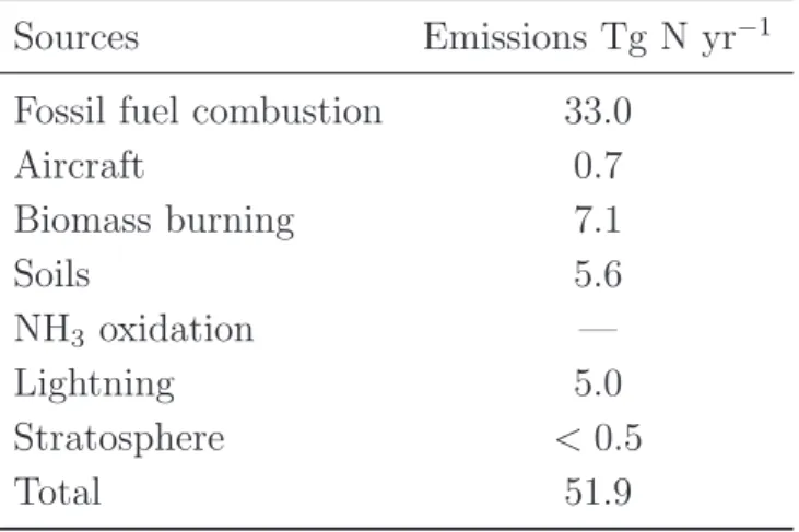
sig-nificant. NOx global emissions estimates are illustrated in table 1.1. The largest source
of NOx is fossil fuel combustion, which explains why these species are more abundant
in urban environments. Atmospheric levels of NOx range from few pptv (∼20 pptv) in
remote areas, such as marine areas and tropical forests, to hundreds of ppbv in polluted urban areas. In rural environments their concentration ranges typically between 0.2 and 10 ppbv (Seinfield and Pandis, 2006). Nitrogen oxides have a major role in tropospheric
processes, which is determining whether VOCs oxidation reactions produce O3 or deplete
it. Indeed, depending on the amount of NO present in the atmosphere, the oxidation reac-tions of VOCs can follow two pathways. In remote environments, where NO concentration
is usually below 50 pptv, O3 is net depleted. When NO is available, like in polluted areas,
where NO concentration can be about 100 ppbv, O3 is formed.
Table 1.1: Estimate of Global Tropospheric NOx Emissions in Tg N yr−1 for Year 2000.
Adapted from Seinfeld and Pandis (2006).
Sources Emissions Tg N yr−1
Fossil fuel combustion 33.0
Aircraft 0.7 Biomass burning 7.1 Soils 5.6 NH3 oxidation — Lightning 5.0 Stratosphere < 0.5 Total 51.9
6 Chapter 1. Introduction to total OH reactivity
1.1.4
Volatile Organic Compounds (VOCs)
The term VOCs refers to the total organic volatile fraction, excluding CO, CO2and CH4. It
includes thousands of different compounds, an unspecified number estimated to be around
104- 105. Their abundance has largely and rapidly increased over the past 200 years,
mainly due to human activities, as combustion of fossil fuels, biomass burning, industrial and agricultural activities and deforestation. Determining the exact composition and atmospheric abundance of this fraction of compounds are main challenges in atmospheric science because of their amount in traces and fast reaction rates towards the atmospheric oxidants. This section aims at providing some general information on the sources and sinks of these compounds.
Sources
Organic compounds are released into the atmosphere through processes associated with life, such as the growth, maintenance and decay of plants, animals and microbes. The com-bustion of living and dead organisms, such as fossil-fuel comcom-bustion and biomass burning are also sources of VOCs.
Organic compounds enter directly the atmosphere through natural and anthropogenic activities. In this way, VOCs are regarded as biogenic VOCs (BVOCs) and anthropogenic VOCs (AVOCs). There is also another important class of VOCs, regarded as oxygenated VOCs (OVOCs), which includes compounds having an oxygen atom in their structure. They can be of both natural and anthropogenic origin, and can enter the atmosphere directly through primary emission or because they are generated from oxidation reactions occurring in the atmosphere, hence secondary produced.
Natural activities are responsible of the emission of the largest majority of VOCs on a global scale (90%), while anthropogenic activities account only for a minor part of these emissions (10%). Globally, anthropogenic activities account for approximately 100 TgC/year of emissions, (Singh and Zimmermann, 1992). Regionally the proportions can be different, for example European anthropogenic and biogenic VOCs are more comparable in magnitude: biogenic emissions are estimated at ∼14 TgC/year, and man-made around 24 TgC/year (Simpson et al., 1999).
Among the anthropogenic sources, road transport, wood burning and solvent use account for 36 TgC/year, 25 TgC/year and 20 TgC/year globally respectively (see table 1.2). Anthropogenic VOCs include alcohols, short and long chain alkanes, alkenes, dienes, alkynes, aromatics, substituted aromatics, esters, ethers, aldehydes, ketones, acids and
others (see Fig. 1.2). Industrial emissions for instance are mainly composed by short and
7
Table 1.2: Estimated global emissions of VOCs (TgC/year) for different anthropogenic sources (adapted from Middleton et al., (1995)
Activity Emissions (Tg yr−1)
Fuel Production / Distribution
Petroleum 8 Natural gas 2 Oil refining 5 Gasline distribution 2.5 Fuel consumption Coal 3.5 Wood 25
Crop residues (including waste) 14.5
Charcoal 2.5
Dung cakes 3
Road transport 36
Chemical industry 2
Solvent use 20
Uncontrolled waste burning 8
Other 10
Total 142
are mainly composed by alkenes, aromatics and acids.
On the other hand, major sources of biogenic VOCs are forests (821 TgC/year), crops (120 TgC/years), shrubs (194 TgC/year), oceans (5 TgC/year) and others (9 TgC/year), accounting for a total estimate of emissions of 1150 TgC/year (Guenther et al., 1995). Plants emit BVOCs for many reasons; e.g. to protect against oxidative stress, to protect against bacteria, as a blossom hormone, for thermotolerance, to defend against herbivores attacks, as antioxidant when exposed to high ozone levels, for signaling (Kesselmeier et
al., 1998 ; Laothawornkitkul et al., 2009). Figure 1.3 gives to the reader an idea of the
number and type of VOCs and the origin of their emission from plants.
Biogenic VOCs include isoprenoids (isoprene, monoterpenes, sesquiterpenes etc.), alkanes, alkenes, alcohols, carbonyls, esters, ethers and acids (Kesselmeier and Staudt, 1999). Iso-prenoids are composed by carbon skeletons of C5 units, depending on the number of units
8 Chapter 1. Introduction to total OH reactivity
Figure 1.2: Chemical structures of some common anthropogenic VOCs.
Figure 1.3: Simplified schematic of biogenic VOCs emissions pathways (adapted from Fall et al., (1999))
they are classified into hemiterpenes (like isoprene C5H8), monoterpenes (C10, like pinenes,
terpinenes, limonene), sesquiterpenes (C15, like caryophyllene), up to polyterpenes with
more than C45 units. Figure 1.4 shows the chemical structure of a number of different
isoprenoids.
Isoprene (C5H8, upper left) is quite unique among all the BVOCs for its dependence to
photosynthetic activity in a plant. It is emitted from a large variety of deciduous plants when photosynthetically active radiation is present, and increases when air temperature also increases. On the other hand, terpenes emissions are linked to the biophysical pro-cesses associated with the amount of material stored in leaf oils and resins and the vapor pressure of the compound itself. Therefore, terpenes emissions do not strongly depend on light and can continue overnight, but they strongly vary with air temperature.
Interest-9
Figure 1.4: Chemical structures of some common biogenic VOCs.
ingly, every plant species emits its characteristics BVOCs: for instance two species of the oak family, Quercus pubescens and Quercus Ilex are respectively a strong isoprene emitter and a terpenes emitter (Kesselmeier et al., 1998). This species-dependent behavior adds additional challenges for estimating BVOCs emissions into the atmosphere. Estimates can be obtained for instance considering the source of emission (Leaf Area Index of the veg-etation), the meteorological parameters activating the emissions and species composition (Megan v.2.1, Guenther et al., 2012).
Isoprene alone is estimated to make almost the half of the total BVOCs emitted (about 594 TgC/year, varying between 520-672 TgC/year), followed by methanol (130±4 TgC/year), monoterpenes (95±3 TgC/year), acetone (37±1 TgC/year), sesquiterpenes (20±1 TgC/year) and other reactive VOCs (96 TgC/year) (Sindelarova et al., 2014).
Global estimates of isoprene have been provided through several approaches, including inverse modelling from transport models and satellite data of formaldehyde, formalde-hyde measurements and bottom-up emissions calculated from detailed regional vegetation descriptions. Within the same approach, based on bottom-up emissions, a factor 3 of difference exists for Europe. When more than an approach is also included, estimates are constrained within 400 and 700 Tg/year. Such result highlights that our current under-standing on the emission of the most abundant VOC is still very poor (see Sindelarova et al., (2014)).
10 Chapter 1. Introduction to total OH reactivity
Table 1.3: Estimated global emissions of some common biogenic VOCs (adapted from Sindelarova et al., (2014))
Global total species mean TgC yr−1
isoprene 594±34 sum of monoterpenes 95±3 α-pinene 32±1 β-pinene 16.7±0.6 sesquiterpenes 20±1 methanol 139±4 acetone 37±1 ethanol 19±1 acetaldehyde 19±1 erbene 18.1±0.5 propene 15.0±0.4 formaldehyde 4.6±0.2 formic acid 3.5±0.2 acetic acid 3.5±0.2 2-methyl-3-buten-2-ol 1.6±0.1 toluene 1.5±0.1
other VOC species 8.5±0.3
CO 90±4
The processes of removal of VOCs from the atmosphere include chemical and physical pro-cesses and their rate of efficiency depends on the physico-chemical properties of the specific chemical compound. Assuming an air parcel containing a generic compound, this organic compound can be simultaneously affected by the following removal processes: (i) oxidation reaction with any of the atmospheric major oxidants, (ii) photolysis by solar radiation, (iii) transport to the stratosphere, (iv) deposition onto surfaces, (v) partitioning into the particle phase. The average of the life histories of all molecules of the mentioned compound yields an average lifetime or the so-called averaged residence time of the compound. For instance, from
A + OH−→k products, (R 8)
11 we can derive τOH = [A] k[OH][A] = 1 k[OH] (1.1)
Considering all the processes affecting the removal of a species in the atmosphere the residence time can be quantified as:
τ = 1
kc + kph+ kt+ kd+ kpa
(1.2)
With kc, kph, kt, kd, kpa being the first order loss rate of A due to chemical reactions,
photolysis, transport, deposition and partitioning into the particle phase. The importance of one removal process compared to one another depends on many factors, included the physico-chemical properties of the considered species, e.g. its rate constant of reaction with one oxidant, its vapor pressure, and its absorbance of UV and visible light. Generally, oxidation reactions constitute the most important sink for VOCs. For instance, BVOCs are all highly reactive compounds towards all the mentioned atmospheric oxidants since
they are all characterized by olefinic double bonds in their chemical structures (Fig.1.4).
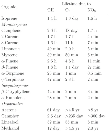
Table 1.4 reports a summary of the residence times for BVOCs as proposed in the review
of Atkinson and Arey (2003), where calculations are performed for [OH]=2 106 molecules
cm−3 [O
3]=7 1011 molecules cm−3 and [NO3]=2.5 108 molecules cm−3. The lifetimes
reported here are only indicative in order to show a ranking of reactivity of the BVOCs. There are indeed many other factors influencing such reactions: time of the day, season, latitude, cloud cover, and the chemical composition of the air mass containing the BVOCs. Isoprene lifetime towards OH is estimated to be only 1.4 hours, while methanol is more stable in the atmosphere and its estimated lifetime with OH is about 12 days. Some monoterpenes and sesquiterpenes, for instance have a residence time of only a few minutes
(α-terpinene has 0.5 min lifetime with NO3 and 1 min lifetime with O3, β-caryophyllene
has 2 min lifetime with O3) therefore their measure in the atmosphere can result very challenging.
In contrast, the atmospheric lifetime of AVOCs is more variable and usually longer com-pared to the biogenic counterpart. Table 1.5 shows a summary of estimated lifetimes for AVOCs as reported in the review of Atkinson, 2000. Estimates were obtained from [OH]=2
106 molecules cm−3 [O
3]=7 1011 molecules cm−3 and [NO3]=5 108 molecules cm−3. For
instance, propane lifetime is calculated to be 10 days with OH, while acetone needs 53 days before it is removed by OH.
12 Chapter 1. Introduction to total OH reactivity
Table 1.4: Calculated atmospheric lifetimes for some common biogenic volatile organic
compounds (BVOCs). Calculations were performed for [OH]=2 106molecules cm−3[O
3]=7
1011molecules cm−3 and [NO
3]=2.5 108molecules cm−3. Adapted from Atkinson and Arey
(2003).
Organic Lifetime due to
OH O3 NO3 Isoprene 1.4 h 1.3 day 1.6 h Monoterpenes Camphene 2.6 h 18 day 1.7 h 2-Carene 1.7 h 1.7 h 4 min 3-Carene 1.6 h 11 h 7 min
Limonene 49 min 2.0 h 5 min
Myrcene 39 min 50 min 6 min
α-Pinene 2.6 h 4.6 h 11 min
β-Pinene 1.8 h 1.1 day 27 min
α-Terpinene 23 min 1 min 0.5 min
γ-Terpinene 47 min 2.8 h 2 min
Sesquiterpenes
β-Caryphyllene 42 min 2 min 3 min
α-Humulene 28 min 2 min 2 min
Oxygenates
Acetone 61 day >4.5 yr >8 yr
Camphor 2.5 day >235 day >300 day
Linealool 52 min 55 min 6 min
Methanol 12 day >4.5 yr 2.0 yr
How strong is the reaction towards one specific oxidant compared to one other is again strictly species dependent (see Atkinson and Arey (2003) and Mogensen et al., (2015)).
For instance, isoprene is more reactive towards OH, followed by its reaction with NO3 and
finally by O3. In contrast, monoterpenes are highly reactive with all the three oxidants,
whereas sesquiterpenes favor the reaction with O3 compared to OH. For the AVOCs
coun-terpart, Formaldehyde needs 1.2 day to be removed by OH and more than 4 years to react with ozone. Propane lifetime with the three oxidants varies even more: it reacts with OH
in 10 days, with NO3 it needs around 7 years and with O3 it is estimated to react in more
than 4500 years.
13
Table 1.5: Calculated lifetimes for some anthropogenic volatile organic compounds
(AV-OCs). Estimates were obtained from [OH]=2 106 molecules cm−3 [O
3]=7 1011 molecules
cm−3 and [NO
3]=5 108 molecules cm−3. Adapted from Atkinson (2000).
Organic Lifetime due to
OH NO3 O3 Photolysis
Propane 10 day ≈ 7 yr >4500 yr
n-Butane 4.7 day 2.8 yr >4500 yr
Ethene 1.4 day 225 day 10 day
Propene 5.3 h 4.9 day 1.6 day
Benzene 9.4 day >4 yr >4.5 yr
Toluene 1.9 day 1.9 yr > 4.5 yr
m-Xylene 5.9 h 200 day > 4.5 yr
Styrene 2.4 h 3.7 h 1.0 day
Phenol 5.3 h 9 min
Formaldehyde 1.2 day 80 day > 4.5 yr 4 h
Acetaldehyde 8.8 h 17 day > 4.5 yr 6 day
Acetone 53 day yr>11 day ≈60 day
abundant VOCs, for instance isoprene on a regional and global scale, emerges that OH,
compared to O3 and NO3, is by far the dominant oxidant.
Oxidation reactions of VOCs usually follow two pathways: (a) addition of the OH radical,
NO3 radical and O3 to the C=C double bonds, (b) H-abstraction from C-H bonds (and
to a lesser extent from O-H bond) by OH radicals and NO3 radicals. Biogenics having
C=C double bonds usually react by addition of the oxidants to the double bonds, while H-abstraction occurs from various C-H bonds of alkanes, ethers, alcohols, carbonyls and esters. The latter is also important for aldehydes, as methacrolein, one of the oxidation products resulting from the oxidation of isoprene.
Figure1.5 shows a simplified schematic of the oxidation reaction of a VOC with any of the
three atmospheric oxidants. When the VOC reacts with OH and NO3, an alkyl radical
(R.) is formed. Then, R. reacts with oxygen forming organic peroxyradicals (RO.
2) and
alkoxyradicals (RO.). The latter can decompose, isomerise, and react with O
2 in the
atmosphere.
Oxidation of VOCs leads to a multitude of different chemical species, whose physico-chemical properties can differ much when compared to their primary precursors. As
14 Chapter 1. Introduction to total OH reactivity
Figure 1.5: Simplified schematic of a volatile organic compound. Adapted from Atkinson (2000).
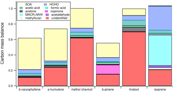
biogenic compounds (Goldstein and Galbally, 2007). Isoprene oxidation products in-clude: formaldehyde, formic acid, acetic acid, acetaldehyde, MVK+MACR, methylfuran, a smaller percentage ends up in the particle phase, while a portion of gaseous products was not identified. This portion refers to a group of masses observed from mass spectrometry analysis which could not been properly identified.
As described in this section, there is a general lack of understanding linked to VOCs pro-cesses. Uncertainties are associated to their emissions and functioning, their atmospheric abundance and composition, the transformation as well as the removal of these species from the atmosphere. Considering just isoprene: it is the largest emitted and most stud-ied non-methane hydrocarbon, it is extremely active in the atmosphere since it can fast react with OH, but estimates on its global emission provided during the last decade are poorly in agreement among them. Measurements of VOCs in ambient air are performed to better elucidate the atmospheric composition and concentration of different environments. However, many challenges arise when measuring VOCs concentration. First, they are a multitude of different species. Recent estimates have reported a large number of
differ-ent organics presdiffer-ent in nature, something around 104-105 (Goldstein and Galbally (2007)).
1.2. Total OH reactivity: a change in philosophy 15 1.0 0.8 0.6 0.4 0.2 0.0
Carbon mass balance
b-caryophyllene a-humulene methyl chavicol b-pinene linalool isoprene
SOA HCHO
acetic acid formic acid acetone nopinone MACR+MVK acetaldehyde methylfuran unidentified
Figure 1.6: Carbon mass balance calculations for the oxidation products of six biogenic VOCs. Adapted from Goldstein and Galbally (2007).
reactive, meaning that some of these compounds can react fast with atmospheric oxidants and be completely or partially lost before they reach any detector. Consequently, a correct quantification of all these species results impracticable. For this reason, it is important to conceive a unique parameter which can directly quantify the total loading of these reactive atmospheric constituents. Interestingly, all these compounds have a common feature: re-acting with the hydroxyl radical. It is exactly this natural process that all VOCs undergo to move towards the development of a new way of thinking in atmospheric sciences.
1.2
Total OH reactivity: a change in philosophy
A fundamental property of the atmosphere is the total OH reactivity, which is defined as the first order loss rate of reaction of the hydroxyl radical with the compounds present in ambient air and represents the inverse of the OH radical lifetime. OH reactivity indicates the frequency of the oxidation reactions involving the reactive atmospheric constituents and OH. Since OH is the main oxidant, OH reactivity also represents an estimate of the total loading of reactive molecules, those that actively participates in the tropospheric processes to form ozone and SOA altering the Earth’s chemical and physical balances. First estimates of the total OH loss rate were obtained summing the concentration of the individual compounds measured multiplied by their rate coefficient of reaction with OH. This approach turned soon to be unfeasible. Indeed, before 1978, only 606 organic
16 Chapter 1. Introduction to total OH reactivity
compounds were identified in the atmosphere. This number increased to 2857 by 1986,
with more advanced analytical technologies the number increased to 104-105, and it might
be far smaller than the number of compounds which is actually present (Goldstein and Galbally, 2007). It turned soon essential to find an alternative approach to quantify such parameter independently from VOCs. Here is the novelty of the OH reactivity philosophy. It is not required measuring the composition of the atmosphere to the smallest detail when the total loading of active components in the air is known. This type of concept has also been extended to ozone production and SOA formation through parameters as ozone production rate (Cazorla and Brune, 2010) and Potential Aerosol Mass (Kang et al., 2007).
1.2.1
OH reactivity relevance
Measuring the total OH sink directly provides the information of the reactive components existing in ambient air, which, as described above, is an important atmospheric property. However, other important information can be obtained from the same measures of OH reactivity. Here below are summarized the main points that make such parameter essential to improve our current understanding of atmospheric chemistry:
(i) OH radical sources
Measures of the total OH sink (OH reactivity) are helpful to constrain the total OH source when the concentration of the hydroxyl radical is known:
[OH] = POH
ROH
(1.3) This approach was used by Whalley and coworkers (2011) for values of OH reactivity and OH concentration measured in the tropical rainforest of Borneo. In their work they stress the presence of an additional OH source when the OH production rates, sink and OH measurements are compared. They found that OH in the tropics is produced at a rate 10 times greater than the identified OH source. Predictions of OH concentration further highlighted that this parameter is underestimated by measures, with important consequences in the degradation of VOCs and methane lifetime over the tropics.
(ii) Unmeasured atmospheric constituents
Measures of OH reactivity can be performed together with measures of ambient air con-stituents. The former is generally regarded as ”measured total OH reactivity”, while the latter is used to calculate the OH reactivity from the summation of the concentration of the individual species multiplied by their rate coefficient with OH (eq. 1.4 and ap-pendix for some references on reaction rate coefficients). The latter is therefore regarded
1.2. Total OH reactivity: a change in philosophy 17
as ”calculated OH reactivity”.
R =X
i
ki+OH·Xi (1.4)
In an ideal environment where every single air component is known in detail the measured OH reactivity and the calculated OH reactivity are the same. If the calculated OH reac-tivity results smaller than the measured OH reacreac-tivity, then a fraction of the composition of the air results unidentified. This fraction is usually regarded as ”missing OH reactiv-ity”. Missing OH reactivity was found to different extents in many environments where measures of OH reactivity were conducted (Di Carlo et al., 2004; Yoshino et al., 2006; N¨olscher et al., 2012). This approach can be used to isolate different cases and improve our current understanding on environmental and atmospheric processes (see Sect. 1.2.4). (iii) Ozone production potential
Rate of instantaneous ozone production potential and regimes can be derived from mea-sures of OH reactivity when associated to measurements of NOx, OH and peroxyradicals. Sinha and coworkers (2012) developed this type of approach to analyse the impact of point sources on regional ozone levels during a campaign in a coastal site in Spain. They found out that the ozone production potential was higher when the coastal site was more influenced by continental air masses. They also identified the point sources that were lim-iting such effect. Their findings demonstrate how significant could be to improve regional
monitoring networks with OH reactivity measurements aside with measures of NOx and
O3, in order to develop the right environmental policies to improve the air quality.
(iv) Particles formation
OH reactivity offers a direct link between VOCs emission/production and particles for-mation. Mogensen et al. (2011) analysed the particles formation events occurred during one month of field campaign in the Finnish boreal forest with the measured data set of OH reactivity. They found out that the missing OH reactivity increased during the particle formation event. Correlations between measured and missing reactivity with the condensation sink confirmed that the missing reactivity could not be explained by OH loss on particles surface, but rather by OH oxidation with VOCs to form higher oxidized semivolatile compounds. Simultaneous measurements of gas phase chemical composition, particle phase chemical composition and OH reactivity would provide some hints to elu-cidate the process of particle formation.
18 Chapter 1. Introduction to total OH reactivity
1.2.2
Measuring the OH reactivity
In 1993, William H. Brune conceived for the first time the concept of total OH reactivity as the direct measure of OH loss rate. A few years later the first measurements of total OH reactivity were performed independently by two research groups in the laboratory based on LIDAR (Calpini et al., 1999) and in ambient air based on laser induced fluorescence for detecting OH (Kovacs and Brune, 2001).
Currently, the total OH reactivity can be measured directly using three different methods: (i) Total OH Loss Rate Measurement (TOLRM) (Kovacs and Brune, 2001; Mao et al., 2009; Hansen et al., 2014); Pump and probe technique (Calpini et al., 1999; Sadanaga et al., 2004; Yoshino et al., 2006; Ingham et al., 2009; Lou et al., 2010) and Comparative Reactivity Method (CRM) (Sinha et al., 2008; N¨olscher et al., 2012a; Dolgorouky et al., 2012; Kim et al., 2011; Kumar and Sinha, 2014).
Total OH Loss Rate Measurement was first developed by Kovacs and Brune (2001). It consists of a flow tube used to sample ambient air at flow rates in the order of 50-400 sL
min−1, wherein a large amount of OH is added through a movable injector. OH
concentra-tion is quantified at different reacconcentra-tion times using a FAGE apparatus (Fluorescence Assay by Gas Expansion, see Faloona et al., (2004) and Dusanter et al., (2009)) at the exit of the flow tube by moving the injector. A decay curve for OH is obtained due to a change in distance between the OH source and the OH detector.
The pump and probe technique was first pioneered by Calpini et al., (1999) and Jeanneret et al., (2001) and then adapted with some differences by other groups (Sadanaga et al., 2004, Yoshino et al., 2006; Ingham et al., 2009 and Lou et al., 2010). The instrument consists of three main parts: a flow tube to sample ambient air, a pulsed laser to generate OH in the sampling reactor, and a FAGE apparatus to quantify OH. The sampling flow is
set around 10-20 sL min−1 and assuming laminar flow the sample has about 1 s residence
time for reaction with OH. The hydroxyl radical OH is generated inside the reactor from ozone photolysis. The decay of OH is measured considering the summed laser pulses using the FAGE instrument.
The Comparative Reactivity Method was more recently developed (Sinha et al., 2008) and then adopted by several research groups in the last decade (Kim et al., 2011; Dolgorouky et al., 2012; Michoud et al., 2015). The popularity of this method comes from the use of analytical techniques such as gas chromatography and mass spectrometry, already in use by many research groups working in the field of the atmospheric sciences. Indeed, in CRM a small glass flow reactor is coupled to a detector such a Proton Transfer Reaction Mass Spectrometer (PTR-MS) or a Gas Chromatography Photo-Ionization Detector (GC-PID).
1.2. Total OH reactivity: a change in philosophy 19
The chosen detector monitors the concentration of a reference molecule, whose reactivity with OH is well known, throughout different experimental stages. The reference molecule, so far always pyrrole, is first diluted in clean air, then reacts with OH radicals generated inside the reactor, then competes for the OH radicals when ambient air is sampled. The competition between pyrrole and reactants in ambient air for OH is acquired in real time, while data processing produces raw data of reactivity with a time resolution of about 10 minutes. Since the CRM is the technique adopted for my PhD project, an exhaustive description of the method can be found in the experimental chapter of this thesis.
Table 1.6: Performance of instruments based on the three existing methods for measuring OH reactivity (modified from N¨olscher et al., 2012).
Method Uncertainty LoD Time Sampling Best main
resolution flow application reference
[%] [s−1] [s] [sL min−1]
TOLRM 10-12 1-2 30-180 50-400
Laboratory studies, Kovacs and
permanent/longterm Brune,
monitoring (2001)
Pump
16-25 1 210 10-20
Laboratory studies, Sadanaga et
and permanent/longterm al., 2004
probe monitoring
CRM 16-35 3-4 10-60 0.3 Forests, Sinha et al.,
chamber studies 2008
Table 1.6 illustrates the differences among the three methods. A comparison of the meth-ods is also provided in N¨olscher et al., (2012a). The methmeth-ods operating with a FAGE have a lower limit of detection (LoD) and report generally a lower uncertainty than CRM, but need larger sampling flows to operate. The CRM has the great advantage of a much smaller sampling flow needed, which broadens its application also to small chambers and branch enclosures experiments. Besides, it is designed to operate on the field. Its size is smaller and more portable than the two other instruments. In addition, it does not operate with a laser and lenses/mirrors that require additional time to be adjusted before performing well. Hence, the CRM can operate easily in the laboratory as on the field. The main drawback of the method consists in the intensive data processing for correcting the raw data for the interferences of the method. It results therefore less elaborated to operate the method in those environments where some of these corrections can be avoided, i.e. in
forests for instance, where NOx concentration is low. Furthermore, the CRM consists of a
20 Chapter 1. Introduction to total OH reactivity
is to use the same instrument to perform both ambient gas phase measurements and OH reactivity (Kumar and Sinha (2014)).
1.2.3
OH reactivity in the world
Measurements of OH reactivity were performed so far at four different scales: (i) in branch enclosures/plant cuvettes (Kim et al, 2011; N¨olscher et al., 2013); (ii) in flow tubes and environmental chambers (Nakashima et al., 2012; N¨olscher et al., 2014); (iii) ground-based ambient measurements (e.g. Ren et al., 2003; Lee et al., 2010; Edwards et al., 2013) and (iv) airborne measurements (Mao et al., 2009).
Ground-based measures were conducted in different environments from different parts of
the world. Fig. 1.7 illustrates the different sites in the world where the OH reactivity
was measured. Green, gray and blue frames represent the type of environment where the measures were performed: i.e. forests, urban and coastal areas, respectively. Bold red
font is used to highlight the sites where a maximum OH reactivity>50 s−1 was observed.
Finally the star indicates the measurements that were conducted with the Comparative Reactivity Method.
Different sites have been investigated so far: observations are reported for urban, forests, rural and remote environments. Forests of different climatic areas were analysed: boreal, temperate, mixed and tropical forests. Most of the measurements reported in literature
were conducted, for logistical reasons, in northern hemisphere as can be seen in Fig. 1.7.
However, measurements at tropical sites in Suriname and Borneo are also reported in literature (Sinha et al., 2008 and Edwards et al., 2013, respectively) and soon will be available the results of the first measures of OH reactivity in the pristine Amazonian rainforest.
Figure1.7 permits to conclude:
• In only 15 years since the development of the first measurements of OH reactivity,
a great effort for measuring this parameter and improving our understanding on atmospheric processes at different sides of the world has been made.
• Many interesting areas of the world are still unexplored: no measures of OH reactivity
existed before my thesis project in the Mediterranean basin, no measures are reported in pristine areas of Asia and Africa, in the Siberian boreal forest, in densely populated urban areas as New Delhi, and in clean remote environments as the poles.
• The magnitude of OH reactivity does not depend on the method used to measure it.
1.2. Total OH reactivity: a change in philosophy 21
existing methods were applied (it is the case for the studies conducted in Mexico city and Paris, using respectively the TOLRM and CRM methods).
• Urban and forest sites are the environments better characterized. However, there is
more variability in type of emission in forests than in urban sites, which means that we could explore more and more forested areas and still miss much information. Be-sides, unknowns on oxidation processes exist at different levels, generating more and more complex systems, e.g. primary reactants emitted from different plant species, secondary species formed from the primary biogenic precursors, interaction between biogenic precursors and anthropogenic components for the ecosystem influenced by pollution.
• Highest values of OH reactivity were reported in megacities and tropical forests
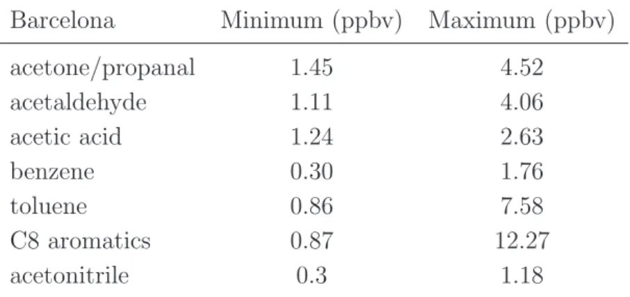
(red highlighted sites). Despite being marked as a coastal area, maximum of OH reactivity at El Arenosillo (Spain) were observed when the site was influenced by continental pollution plumes from big cities as Madrid and Sevilla. Maximum values
of OH reactivity observed in megacities are alarming: 200 s−1 in Mexico City during
spring 2003 (Shirley et al., 2006); 130 s−1 in Paris during winter 2010 (Dolgorouky
et al., 2012); 100 s−1 in Tokyo during autumn 2004, in New York City during winter
2004 and in Beijing during summer 2006 (Yoshino et al., 2006; Ren at el., 2006; Lu et al., 2013). In tropical forests local drivers as higher ambient temperature and solar radiation trigger the emissions of BVOCs, resulting in a more intense photochemistry, therefore higher OH reactivity compared to temperate environment.
• The magnitude of OH reactivity depends mainly on the type of environment but
also on the season of measurements. Observations conducted in forested sites report a clear seasonal dependence, with the OH reactivity being larger in during spring and summer. Observations conducted in urban sites, as Tokyo, during all seasons
provide an example: wintertime maximum OH reactivity was slightly below 50 s−1,
22 C h a p te r 1 . In tr o d u ct io n to to ta l O H re a ct iv it y
Figure 1.7: OH reactivity measurements world map. Arrows indicate the sites where measurements of OH reactivity using the three different experimental methods were conducted. Green, gray and blue frames refer to forested, urban and coastal sites. Red font indicates the sites where a maximum value of OH reactivity>50 s−1 was reported. The star indicates
1.2. Total OH reactivity: a change in philosophy 23
1.2.4
The missing OH reactivity
The missing OH reactivity is simply the fraction of reactivity which is not explained by the simultaneous measurements of concentration of gaseous atmospheric constituents. In other words, it corresponds to the unmeasured compounds in ambient air. These com-pounds can be unmeasured for three main reasons:
(i) they are not measured because of the lack of an appropriate technique for measuring them;
(ii) they are measured but their contribute to the OH reactivity is not known due to tech-nical issues for identifying the species or to the not known kinetics of reaction;
(iii) they are not measured because they are not known to exist.
It is especially this last hypothesis that has contributed considerably to pose the interest on the OH reactivity parameter. It is this last hypothesis to make us confident that there are more species in air than those measured or estimated to be (Goldstein and Galbally, 2007).
It is difficult to compare studies of OH reactivity using different methods, deployed by different operators while the suite of complementary measures available in the gas phase is different. Therefore comparisons among missing reactivity provided by different works have to be taken with caution. However, OH reactivity in forests have shown so far the largest gaps between OH reactivity measured and calculated. Those values are larger than in urban environments, for instance.
Di Carlo and coauthors (2004) were the first to show evidences for unknown reactive BVOCs in a temperate forest in Michigan. They showed that the missing reactivity in this forest had the same temperature dependency as terpenes and concluded that the unmeasured compounds were unknown terpene-like species. Kim et al. (2011) measured for the first time the OH reactivity in plant cuvettes. They isolated a few plant species to see if their emissions were completely characterized. Indeed plant cuvettes are perfect means to help disentangling the origin of the missing reactivity. They saw that the few plant species investigated were emitting compounds whose concentration was measured by their techniques. Hence they concluded that the missing OH reactivity has mainly a secondary origin. N¨olscher et al., (2012) measured the OH reactivity in the Finnish boreal forest, during a warmer than usual summer. Their missing reactivity was almost 90% and they attributed it to species emitted as a consequence of heat stress on trees.