HAL Id: tel-01795097
https://tel.archives-ouvertes.fr/tel-01795097
Submitted on 18 May 2018
HAL is a multi-disciplinary open access archive for the deposit and dissemination of sci-entific research documents, whether they are pub-lished or not. The documents may come from teaching and research institutions in France or abroad, or from public or private research centers.
L’archive ouverte pluridisciplinaire HAL, est destinée au dépôt et à la diffusion de documents scientifiques de niveau recherche, publiés ou non, émanant des établissements d’enseignement et de recherche français ou étrangers, des laboratoires publics ou privés.
Abbass Zein Eddine
To cite this version:
Abbass Zein Eddine. Algorithmes de détection et diagnostic des défauts pour les convertisseurs sta-tiques de puissance. Autre. Normandie Université; Université Libanaise. Faculté des Sciences (Bey-routh, Liban), 2017. Français. �NNT : 2017NORMLH28�. �tel-01795097�
THESE
Pour obtenir le diplôme de doctorat
Spécialité (GENIE INFORMATIQUE ET AUTOMATIQUE)
Préparée au sein des laboratoire GREAH (Groupe de Recherche En Electrotechnique Et Automatique Du Havre – EA 3220) de l'Université du Havre
En partenariat international avec Université Libanaise - Liban
Algorithmes de détection et diagnostic des défauts pour les
convertisseurs statiques de puissance
Fault detection and diagnosis algorithms for power converters
Présentée et soutenue par Abbass ZEIN EDDINE
Thèse dirigée par Prof. Dimitri LEFEBVRE et co-directeur Dr. François GUERIN, laboratoire GREAH Thèse dirigée par Prof. Abbas HIJAZI et co-directeur Dr. Iyad ZAAROUR, laboratoire LPE
Thèse soutenue publiquement le (20/06/2017) devant le jury composé de
Cecile LABARRE Professeur Rapporteur Hassan NOURA Professeur Rapporteur Bilal SAEED Docteur Examinateur Abbas HIJAZI Professeur Director Dimitri LEFEBVRE Professeur Director Francois GUERIN Docteur Co-Director Iyad ZAAROUR Docteur Co-Director
This thesis is dedicated to my parents, Mr. and Mrs. ZEIN EDDINE.
To my beloved future wife Fatima.
I would like to express my sincere gratitude to my advisor prof. Dimitri Lefebvre for the continuous support of my PhD study and related research, for his patience, motivation, and immense knowledge. His guidance helped me in all the time of research and writing of this thesis. I could not have imagined having a better advisor and mentor for my PhD study.
I would like to thanks Dr. Iyad Zaarour, who was the reason for this thesis. I appreciate his guidance throughout this study. Many of the new ideas are developed through the discussion with him. You have made a great influence on my life. You are more than a mentor, you will always be a family member.
Special thanks to Dr. Franҫois Guerin for your valuable technical support. Thanks for sharing your experience and knowledge. All these results were not to be without your help. I really appreciate your hard work to complete my thesis.
I would also like to thank Prof. Abbas Hijazi. The door to Prof. Hijazi office was always open whenever I ran into a trouble spot or had a question about my research or writing. He consistently allowed this work to succeed, but steered me in the right direction whenever he thought I needed it.
Special thanks for the Lebanese University and the CNRS for the PhD funding. This accomplishment would not have been possible without them. Thank you.
I must express my very profound gratitude to all my family members, especially my parents: Hassan Zein Eddine and Batoul Alawieh, for providing me with unfailing support and continuous encouragement. They followed me since I was born and helped me carry my projects until its completion. They supported me with all their love and this stage is also theirs. They have given me everything and I owe them everything.
And most of all for my loving, supportive, encouraging, and patient fiancée Fatima Alawieh whose faithful support during the entire stages of this PhD was my caring map to success.
Last, but certainly not least, praise be to Allah who made praise the key for His remembrance. I will keep on trusting you for my future.
DC-DC converters have received significant interest recently as a result of their high power capabilities and good power quality. They are of particular interest in systems with multiple sources of energy. However due to the large number of sensitive components including power semiconductor devices, coils, and capacitors used in such circuits there is a high likelihood of component failure.
This thesis considers one of the most promising DC-DC converters—the ZVS full bridge isolated Buck converter. An approach with two stages is presented to detect and isolate open-circuit faults in the power semiconductor devices in systems with DC-DC converters. The first stage is the fault detection and isolation for a single DC-DC converter, while the second stage works on a system with multiple DC-DC converters. The proposed methods are based on Bayesian Belief Network (BBN). The signals used in the proposed methods are already available as measurement inputs to control system and no additional measurements are required. An experimental ZVS full bridge isolated Buck converter has been designed and built to validate the fault detection and isolation method on a single converter. The methods can be used with other DC-DC converter typologies employing similar analysis and principals.
Keywords: DC-DC converters, Fault Detection and Isolation, Bayesian Belief Network,
Les convertisseurs DC-DC suscitent un intérêt considérable en raison de leur puissance élevée et de leurs bonnes performances. Ils sont particulièrement utiles dans les systèmes multi-sources de production d'énergie électrique. Toutefois, en raison du grand nombre de composants sensibles utilisés dans ces circuits et comprenant des semi-conducteurs de puissance, des bobines et des condensateurs, une probabilité non négligeable de défaillance des composants doit être prise en compte.
Cette thèse considère l'un des convertisseurs DC-DC les plus prometteurs - le convertisseur ZVS à pont isolé de type Buck.
Une approche en deux étapes est présentée pour détecter et isoler les défauts en circuit ouvert dans les semi-conducteurs de puissance des convertisseurs DC-DC. La première étape concerne la détection et la localisation des défauts dans un convertisseur donné. La seconde étape concerne sur les systèmes munis de plusieurs convertisseurs DC-DC. les méthodes proposées sont basées sur les réseaux Bayésiens (BBN). Les signaux utilisés dans ces méthodes sont ceux des entrées de mesure du système de commande et aucune mesure supplémentaire n'est requise. Un convertisseur expérimental ZVS à pont isolé de type Buck a été conçu et construit pour valider la détection et la localisation des défauts
Sur un seul convertisseur. Ces méthodes peuvent être étendues à d'autres types de convertisseurs DC-DC.
Mots clés: Convertisseurs DC-DC, Détection et isolation des défauts, Réseau Bayésien, Observateur
ACKNOWLEDGEMENTS 5 ABSTRACT 7 RESUME 9 LIST OF FIGURES 15 LIST OF TABLES 17 CHAPTER 1 : INTRODUCTION 19 1.1 Motivation 19 1.2 Contribution 20 1.3 Thesis Structure 22 CHAPTER 2 DC-DC CONVERTERS 25 2.1 Introduction 25
2.2 Different classes of DC-DC converters 26
2.3 Zero Voltage Switch (ZVS) full bridge isolated Buck converter 31
2.3.1 Operation 32
2.3.2 State space model 34
2.4 Reliability in static converters 40
2.4.1 MOSFET faults 41
2.4.2 Inductor faults 41
2.4.3 Diode faults: 42
2.4.4 Capacitor faults: 42
2.5 Considered faults 42
2.5.1 MOSFET transistor (Q1) open-circuit fault model (fault 1) 43
2.5.2 Diode (D8) open-circuit fault model (fault 2) 44
2.5.3 Coil (L) open-circuit fault model (fault 3) 44
3.2 Fault detection and isolation 47
3.2.1 Hardware (physical) FDI 48
3.2.2 Software (analytical) FDI 49
3.3 Fault detection and isolation in DC-DC converters 51
3.4 Bayesian Belief Network (BBN) in FDI 58
3.4.1 Bayesian belief network 58
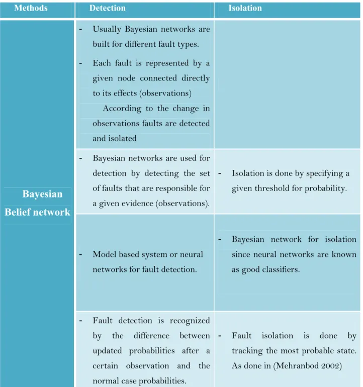
3.4.2 BBN in fault detection and isolation 61
3.5 Conclusion 68
CHAPTER 4 FAULT DETECTION AND ISOLATION USING BBN IN DC-DC
CONVERTERS 69
4.1 Introduction 69
4.2 FDI using Bayesian Naïve Classifier (BNC) in single DC-DC converter 69
4.2.1 Observer design 69
4.2.2 BBN structure and parameters 71
4.2.3 Experimental results 73
4.3 Conclusion 105
CHAPTER 5 FAULT ISOLATION IN SYSTEM OF MULTIPLE DC-DC CONVERTERS 107
5.1 Introduction 107
5.2 FDI using hierarchical BBN in system of multiple DC-DC converters 107
5.2.1 BBN structure and parameters 107
5.2.2 Experimental results 111
5.3 Conclusion 132
CHAPTER 6 CONCLUSION AND FUTURE WORKS 133
6.1 Conclusion 133
6.2 Future works 134
ANNEX 1: CONTROL LOOPS 137
L
IST OF
F
IGURES
Figure 2.1: Topology of the considered SMSE (Guerin et al. 2012). ... 26
Figure 2.2: Buck converter schematic diagram ( www.learnabout-electronics.org) ... 28
Figure 2.3: Boost converter schematic diagram (www.learnabout-electronics.org) ... 28
Figure 2.4 : Buck-Boost Converter (www.radio-electronics.com) ... 29
Figure 2.5 : Simple Flyback converter circuit ... 30
Figure 2.6 : Push-Pull DC-DC converter structural diagram. ... 31
Figure 2.7 : ZVS full bridge isolated Buck converter structural diagram ... 31
Figure 2.8: Four phases of the DC-DC converter operation ... 33
Figure 2.10: Phase-shift control of the ZVS full-bridge converter. Switching transitions are neglected in this figure... 34
Figure 2.11: Industry based survey of component reliability in static converters (Griffin et al. 2002). ... 40
Figure 3.1: Classification of FDI methods (Patton et al. 1989) ... 48
Figure 3.2: Basic concept of model-based FDI techniques (Yang et al. 2009). ... 50
Figure 3.3: Grid-connected power converter (Kalman 2015). ... 52
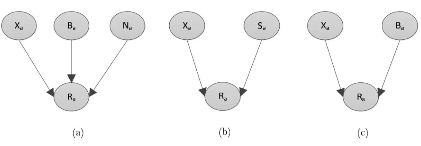
Figure 3.4: (a) model 1, (b) model 2, (c) model 3. ... 62
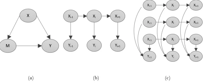
Figure 3.5: (a) GMM, (b) HMM and (c) FHMM. Y represents the observed values that are the input and the output of the system while X represents the system state (hidden). ... 66
Figure 4.1 BNC structure ... 72
Figure 4.2: Direct measurements: (a) MOSFET (Q1) open circuit fault; (b) Diode (D8) open circuit fault; (c) Coil (L) open circuit fault. ... 75
Figure 4.3 Residual variation and alarm generation for FDI method based on observer (fault detection): (a) MOSFET (Q1) open circuit fault; (b) Diode (D8) open circuit fault; (c) Coil (L) open circuit fault. ... 77
Figure 4.4 BNC structure used for isolation ... 78
Figure 4.5: BBN classifications for learning evaluation: (a) for 1 dataset; (b) for 2 dataset; (c) for 3 dataset ... 79
Figure 4.6: BNC classification probabilities for learning evaluation (a) for 1 dataset; (b) for 2dataset; (c) for 3 dataset. ... 81
Figure 4.7: BNC classifications for validation. (a) for 1 MOSFET (Q1) open circuit fault ; (b) for 2 Diode (D8) open circuit fault; (c) for 3 Coil (L) open circuit fault... 83
Figure 4.8: BNC structure (second experiment) ... 84
Figure 4.9: BNC classifications: (a) for 1 MOSFET (Q1) open circuit fault; (b) for 2 Diode (D8) open circuit fault; (c) for 3 Coil (L) open circuit fault ... 85
Figure 4.10: BNC classification probability: (a) for 1 dataset; (b) for 2 dataset; (c) for 3 dataset ... 86
Figure 4.11: ZVS full bridge isolated Buck converter designed by GREAH. ... 87
Figure 4.12: Collected data (a) situation 1 (b) situation 2 (c) situation 3 ... 89
Figure 4.14: Residuals (source current IG, inductance current IL, output voltage S); (a) scenario 1 residuals and detection alarm; (b) scenario 2 residuals and detection alarm; (c) scenario 3 residuals and detection alarm. ... 93 Figure 4.15: BNC classifications: (a) for 1 scenario 1; (b) for 2 scenario 2; (c) for 3 scenario
3; ... 97 Figure 4.16: BNC classification, detection and isolation: (a) scenario1; (b) scenario2; (c)
scenario3; ... 100 Figure 5.1: Generalized BBN structure for faulty converter detection ... 109 Figure 5.2: Generalized BBN structure for fault isolation. ... 111 Figure 5.3: Collected data: (a) fault 1 and 2 in converter 1; (b) fault 3 in converter 1; (c) normal
resource changes for converter 1; (d) fault 1 and 2 in converter 2; (e) fault 3 in converter 2; (f) normal resource changes for converter 2. ... 116 Figure 5.4 Case study BBN structure for faulty DC-DC converter detection ... 119 Figure 5.5: BBN classifications for detecting faulty converter: (a) when fault1 and fault2 in
converter1 occurs; (b) when fault3 in converter1 occurs; (c) when fault1 and fault2 in converter3 occurs; (d) when fault3 in converter2 occurs; (e) during normal changes in converter1 resources; (f) during normal changes of converter3 resources. ... 122 Figure 5.6: BBN classifications confidence for detecting faulty converter: (a) when fault1 and
fault2 in converter1 occurs; (b) when fault3 in converter1 occurs; (c) when fault1 and fault2 in converter3 occurs; (d) when fault3 in converter2 occurs; (e) during normal changes in converter1 resources; (f) during normal changes of converter3 resources. ... 125 Figure 5.7: Case study BBN structure for occurring fault isolation ... 128 Figure 5.8: BBN classifications for isolate the occurring fault in the faulty converter: (a) when
fault1 and fault2 in converter1 occurs; (b) when fault3 in converter1 occurs; (c) when fault1 and fault2 in converter3 occurs; (d) when fault3 in converter2 occurs. ... 131
L
IST OF
T
ABLES
Table 1: Main variables for the DC-DC converter state space model. ... 35
Table 2: Four cases of BN learning problem ... 59
Table 3: The use of BBN in the domain of FDI. ... 67
Table 4. Case study parameters. ... 73
Table 5: Faults signature: the sign of the residuals generated by the proposed observer for the three considered faults. ... 78
Table 6: Evaluation confusion matrix ... 79
Table 7: Belief index (mean of probabilities). ... 81
Table 8: Validation confusion matrix ... 82
Table 9: Confusion matrix... 86
Table 10: The occurrence, detection and delay time ... 93
Table 11: Isolation belief index ... 95
Table 12: Confusion matrices. ... 97
Table 13: Delay for detection with BNC ... 100
Table 14: Confusion matrices. ... 102
Table 15: Isolation belief index ... 103
Table 16: Comparative table: PO Vs BNC. ... 104
Table 17: Faults modeling ... 112
Table 18: Collected datasets and validation sets... 118
Table 19: Confusion matrix for faulty DC-DC converter detection. ... 126
Table 20: Confusion matrix for C1 inference... 132
Abbass ZEIN EDDINE Page 19
Chapter 1
:
I
NTRODUCTION
1.1 Motivation
In the recent decades, electrical energy has constituted the base of most scientific inventions and technological revolutions. As a result, electrical equipment has emerged as an integral part of our daily life leading to a greater demand for electrical energy and, consequently, for reliable electrical supplying systems that supply continuously consumers with electrical energy. On the other hand, the limited reserves of fuel oil and their unstable prices have significantly increased the interest in green energy (photovoltaic modules, wind turbine, PEMFC, etc). Thus, many topologies of hybrid power systems, or Systems of Multiple Sources of Energy (SMSE) were proposed (Guerin et al. 2012, Hui et al. 2010).
To insure the supplying continuity, it is required to have a fault-free process during all the phases of energy production, transfer and conversion. Concerning the conversion phase, energy converters play one of the most important roles in the electric power lifecycle. Therefore in our work we are going to focus on such equipment, especially DC/DC converters. Such converters are used in some topologies of Systems of Multiple Sources of Energy (SMSE) such as the one presented in (Guerin et al. 2012). Those DC/DC converters are used to manage the coupling and decoupling of the energy sources on a DC bus according to the load demand and available power.
In order to improve the system operation and avoid catastrophic consequences, it is mandatory to have a Fault Detection and Isolation (FDI) system that holds on the faulty cases. Power semi-conductors devices are the most voltage sensitive components in a power converter (Yang et al. 2011). In addition those components represent the core of the converters since they play the main roles. Therefore, in the presence of failure of power semi-conductor devices, a DC/DC converter will operate with distorted output voltages and currents. High voltages and currents caused by the failed device may also cause secondary damages to other devices if the faulty operation is allowed and a shutdown of the converter may follow. To
Abbass ZEIN EDDINE Page 20 improve the availability of these converters it is important that any device failure is detected and isolated quickly.
Fault detection and isolation methods are categorized as data-based methods which depend on identifying the system from previously collected data from the system itself, and model-based methods which depend on the mathematical and physical equations of the system and that need a deep understanding of causal relationships between process variables, inputs and outputs. Those methods are responsible to perform two tasks, detecting anomalous situations (fault detection) and addressing their causes (fault isolation) (Caccavale and L. Villani 2002).
In this work two FDI methods are proposed to improve the availability of a ZVS full bridge isolated Buck converters. The methodology in this work is based on a Bayesian Belief Network (BBN). A BBN is a probabilistic graphical model that represents a set of random variables and their conditional dependencies via a Direct Acyclic Graph (DAG). The flexibility of BBN structure and the ability of learning the system dependencies make it a good candidate for application in FDI.
There are two types of failures seen in fully controlled power semi-conductor devices: the short-circuit fault and open-circuit fault. Short-circuit fault are often detected using hardware methods such as de-saturation detection integrated within a gate driver. This work concentrates FDI for open-circuit faults in power semi-conductor devices in DC-DC converters. In addition, this work also considers status monitoring for the coils.
1.2 Contribution
Two methods based on Bayesian Belief Network (BBN) are proposed in this thesis for fault detection and isolation in DC-DC converter. These methods utilize input signals which are already available as measurement inputs to the control system and require no additional measurement elements. These methods are detailed as follows.
• Method 1 is capable of detecting and locating an open circuit fault of a power semiconductor device in a DC-DC converter. A proportional observer is employed to observe the input current, inductance current and output voltage in the DC-DC converter. Normally
Abbass ZEIN EDDINE Page 21 the observer states converge to the corresponding measured states; but in the presence of fault the observed states will diverge from the measured states. The fault can then be detected by comparing the difference between the estimated output by the observer and the measured output of the system with a calculated threshold values. For isolation a simple Bayesian Naïve Classifier (BNC) is introduced since the observer residuals were similar during all the considered faults. This BNC is used in two ways, the first by learning the residuals of the designed observer and consequently benefit from its classifications to isolate the fault, second by learning the state of the system (direct measurements) and benefit from the BNC classifications to locate the fault.
• Method 2 deals with more complex problem than that of method 1. This method detects and isolates faults in system of multiple DC-DC converters. The method is based on Hierarchical Bayesian Network (HBN), which is used for the first time in the domain of FDI in DC/DC converters. First the problem is simplified by dividing it into two parts: (i) detecting the faulty converter, (ii) isolate the occurring fault in the faulty converter. This simplification will reduce the complexity of the BBN structure that will represent the system, in addition to the complexity of the parameters (Conditional Probability Tables (CPTs)) representing the relation between the structure nodes. Thus two BBN structures are specified, the first one is constructed in a way to detect the faulty converter and it will run in parallel with the system and classify the system observations. While the second BBN is built to isolate the fault in the detected converter, this BBN will run directly after the first BBN detect a fault. In this method disturbance and control loops are considered.
Thus we can sum up our work contribution as follow:
(i) The problem of fault detection and isolation is treated from a computer science point of view by using Bayesian belief network as the first time for such task in power converters.
(ii) Compared to previous studies, our algorithm does not require additional measurements and therefore auxiliary components and sensors than those that are usually equipped on the converter.
(iii) Noise and control loops (voltage/ current) are considered which make the task more complex, because noise degrades the quality of captured signals and data, and control loops tries to compensate the faults' effect on the studied signals in a short time.
Abbass ZEIN EDDINE Page 22 (iv) Unlike previous studies a single global method is proposed to detect and isolate faults in system of multiple DC-DC converters this method takes measurements from several converters and give a decision. While in previous studies a method is used for each converter in the system.
(v) The second method (FDI in system of multiple DC-DC converters) is easy to be generalized and extended by just adding nodes for the new converter.
(vi) The second method (FDI in system of multiple DC-DC converters) uses data from all the converters to detect the faulty one.
(vii)The results show good detection time with low delay, less than 10 ms.
It is noted that although only investigated for a Zero Voltage Switch (ZVS) full bridge isolated Buck converter, these two methods can be applied to other DC-DC converters by employing similar analysis and principles.
1.3 Thesis Structure
The thesis is structured as follows.
Chapter 2 gives an overview about the DC-DC converters, and introduces the ZVS full bridge isolated Buck converter topology, plus to the System of Multi-Sources of Energy (SMSE) coupling several sources of energy to a DC-bus via identical DC-DC converters. In addition the state space models representing both systems (single converter and SMSE) are provided. Moreover, the problem of DC-DC converters reliability is discussed. The chapter ends with a summary about the considered faults and the model of the DC-DC converter in normal and faulty operating conditions.
In chapter 3 the Fault Detection and Isolation (FDI) definition, categories, and methods are presented. In addition a state of the art for FDI in DC-DC converters is performed, discussing the previous work done in tackling this problem. This chapter also details and highlights the BBN method and its contributions in the domain of FDI.
In chapter 4 the FDI method 1 is presented. This method can be used to detect and locate an open circuit device fault. The chapter begins with an introduction about proportional observers
Abbass ZEIN EDDINE Page 23 that are previously used as FDI method for DC-DC converters. Then a Bayesian Naïve Classifier (BNC) structure is described which is used to estimate the faulty state of the system depending on the system observations. Based on those two frameworks, an algorithm for fault detection and isolation is introduced. The proposed algorithm and the robustness analysis are validated using simulation and real data results.
In chapter 5 the FDI method 2 is presented. This method deals with the problem of detecting and isolating faults in system of multiple DC-DC converters, with one fault in one converter at a time. Two BBN structures are built, the first one to learn the behavior of the system when one converter is faulty in order to detect the fault. This structure will run in parallel with the system all the time. The second structure is to isolate the fault in the faulty converter detected by the first BBN structure, this BBN will run when the first BBN detects a fault. The detection and isolation are based on the classification of the BBN at several consecutive observations. The proposed algorithm is validated using simulation results with system of two DC-DC converters taking into consideration the control loops that tries to compensate the fault behaviors by controlling the control input of each converter.
In chapter 6 conclusion, potential applications of the proposed techniques and future works are discussed.
Abbass ZEIN EDDINE Page 25
Chapter 2
DC-DC
C
ONVERTERS
2.1 Introduction
Power electronics refer to control and conversion of electrical energy by power semiconductor devices wherein these devices operate as switches. Their applications span the whole field of electrical energy systems especially in the energy conversion. The modern power electronic technology enables various renewable energy sources to produce and interface with DC power directly. Much research on connecting the DC energy sources directly to the DC grid has been carried out extensively (Hammerstrom 2007), (Izadian and Famouri 2010). The DC grid systems have gained more attention again due to the opportunities and advantages they could provide. Figure 2.1 illustrate a topology for a System of Multiple Sources of Energy SMSE (Guerin et al. 2012), where there are multiple sources of energy including conventional and renewable energy sources, connected to a DC bus via identical ZVS full bridge isolated Buck converters. The main role of these converters is to couple and decouple those sources on the DC bus according to the available resources. This work has been studied before in (Guerin et al. 2012) where a supervisory control strategy was proposed in order to manage the operation modes (i.e. to decide the sources that should be coupled and the one that should be decoupled).
Static converters are devices that convert voltage and current from one form to another. Mainly there are four types of static converters: rectifiers (AC-DC converter), inverters (DC-AC converter), choppers (DC-DC converter), and transformers ((DC-AC-(DC-AC converter). A DC-DC converter is one of the most essential components in the DC grid system, because the energy sources are connected to the grid through it. This chapter will give an overview about DC-DC converters operation, because they are the interest of our work, especially the Zero Volt Switch (ZVS) full bridge isolated Buck converter.
Abbass ZEIN EDDINE Page 26 Figure 2.1: Topology of the considered SMSE (Guerin et al. 2012).
2.2 Different classes of DC-DC converters
DC-DC converters are electronic devices that are used whenever DC output voltage needs to be changed from one level to another. This type of static converters is used in many daily life equipment such as cars radio fed by 24 V battery (24V/12V converter), mobile phone battery charged from a car battery (24V/3V converter), electronics devices where a 1.5V from a single cell battery must be stepped up to 5V, or in an sine-wave inverter where a 12V DC must be stepped up to 650V as a part of the DC-AC converter used in the inverter, and many other applications even in some renewable energy systems, as an instance, the hybrid cars that save gasoline by working partially on electrical energy saved in the battery, the satellites that collect energy from by the photovoltaic solar plates, etc.
There are many types of DC-DC converters. Mainly there are two categories, first the non-isolating converters, second the non-isolating converters.
i. Non-isolating converters: in this category there is a direct connection between the DC input and the DC output. They are usually used to step up or step down by a small ratio. There
Abbass ZEIN EDDINE Page 27 are five different sub-categories of non-isolating converters: buck, boost, buck-boost, cuk and charge-pump.
Buck converters or step-down converters are used to reduce the DC input voltage. Figure 2.2-a presents the schematic diagram of the Buck DC-DC converter. This DC-DC converter is formed of a MOSFET transistor, a diode, a capacitor, an inductor and a control circuit that controls the MOSFET gate with a pulse width modulation signal.
This DC-DC converter passes through two phases. The first phase is when the MOSFET is in the ON state. In this case, the source voltage supplies the load and charges the inductor and capacitor. The second phase begins when the MOSFET is turned OFF. In this case, the load will be supplied by the discharging of the inductor and capacitor. The Buck converter continues to alternate between these two phases, and can act in two modes, first, acting in a Continuous Condition Mode (CCM). In CCM the output current is always positive and continuous. Second, acting in a Discontinuous Conduction Mode (DCM), which means that, each OFF switching of the diode is due to a natural decrease of the output current to zero.
The output voltage is then controlled by the duty cycle φ (φ =TON/T) of the signal applied to
the gate of the MOSFET transistor. In CCM, the relation between the input voltage V and output voltage V is V =V × φ.
Boost converters or step up converters are formed of the same components used in Buck converters but with a different combination (Figure 2.3-a). In the first phase the MOSFET transistor is OFF, the voltage delivered to the load is equal to the input voltage plus the inductor voltage (knowing that the inductor is charged from the initial state). Thus the output voltage is greater than the input voltage, and the capacitor is charging by a voltage V = V + V (where V is the source voltage). Now in the second phase the MOSFET transistor is ON. The capacitor will feed the load by V and the inductor will be charged again. The Boost converter will continue to alternate between these two phases. In the CCM, the relation between the input voltage V , the output voltage V , and the duty cycle (φ) of the signal applied to the gate of the MOSFET transistor is as follow = i. e. = .
Abbass ZEIN EDDINE Page 28 Figure 2.2: Buck converter schematic diagram ( www.learnabout-electronics.org)
(a)
Figure 2.3: Boost converter schematic diagram (www.learnabout-electronics.org)
Buck-Boost converter is a combination of the previous two types such that it can work as a step-down converter or a step-up converter depending on the value of the duty cycle of the signal applied to the gate of the MOSFET transistor. The schematic diagram of the Buck-Boost converter is formed of the same components the Buck and Buck-Boost converters formed of as shown in Figure 2.4. When the MOSFET transistor is ON the input current will charge the inductor only and no current will flow through the diode because its reverse biased. In addition the load will be supplied by the capacitor. Then at the next phase the MOSFET transistor is OFF and the inductor starts to supply the capacitor and the load because the inductor reverses its EMF and the diode will become forward biased. With this configuration the ratio between the output V and input V voltages turns out to be: = and = , this means
Abbass ZEIN EDDINE Page 29 that when is greater than the DC-DC converter will work as a Boost converter, else if is greater than (i.e. φ<0.5) the Buck-Boost converter acts as a Buck converter. Moreover the minus indicates that a Buck-Boost converter is able to change the polarity of the output voltage since the output voltage is the inverse of the input one.
Figure 2.4 : Buck-Boost Converter (www.radio-electronics.com)
ii. Isolating converters: in the majority of applications, it is desired to incorporate a transformer into the DC-DC converter, to obtain galvanic isolation between the DC-DC converter input and output or to increase the voltage output level. For example, in off-line power supply applications, isolation is usually required by regulatory agencies. There are several types of isolating converters.
The Flyback converter ( Figure 2.5) is formed of the same components as previous topologies but a transformer is used instead of an inductor to store the energy. This circuit alternates between two phases. First, the MOSFET transistor is ON, the current flow through the primary winding of the transformer and stores energy while the capacitor feds the load. Then the second phase starts by turning OFF the MOSFET transistor, in this case the energy stored in the primary winding will transfer into a current in the second.
In this topology the relation between input and output voltage doesn’t depend only on the number of turns in the windings of the transformer (L2/L1) even that it plays an important role in stepping-up voltage, but also on the duty cycle value of the signal applied to the gate of
Abbass ZEIN EDDINE Page 30 the MOSFET transistor. = .(L2/L1).( / ) where L2 is the number of turns in the
secondary winding of the transformer and L1 is the number of turns in the primary winding.
Figure 2.5 : Simple Flyback converter circuit
Forward DC-DC converters work in contrast to the Flyback because there is no energy stored in the primary winding at first phase and then transferred again into current at the second winding at the second phase. Forward DC-DC converters are those that convert the DC input into an intermediate AC supply and then use a rectifier to get a final DC output, because the energy in AC form is simply treated and adapted. There are many types of forward DC-DC converters, for example, the push-pull converter (Figure 2.6). In push-pull converter, the energy is directly transferred between the input and output in one step. This is done by using two MOSFET transistors and a center tapped transformer. These two MOSFET transistors are turned ON and OFF alternately i.e. they are never ON together. The DC current is turned into AC current by alternating between two cases. The first is when MOSFET transistor 1 and 2 are respectively ON and OFF, the current flow through the first half of the primary winding. The second is when MOSFET transistor 1 and 2 are respectively OFF and ON, the current starts to flow through the second half of the primary winding. The alternating between these two cases in a fast manner leads to an induced current in the secondary winding and the current flows in the second part of the circuit. After that this current is rectified into a DC current using a full-bridge of diodes and delivered to the capacitor and load. The output current may be stepped-up or down by the means of the transformer by increasing the number of turns in the second winding. The output voltage is: Vout=Vin × (L2/L11) while L2 is the number of turns in the second winding and L11=L12 are the halves of the primary winding.
Abbass ZEIN EDDINE Page 31 Figure 2.6 : Push-Pull DC-DC converter structural diagram.
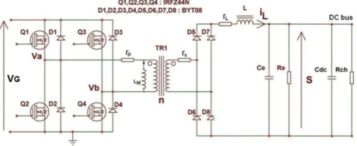
2.3 Zero Voltage Switch (ZVS) full bridge isolated Buck converter
ZVS full bridge isolated Buck converter structural diagram is shown on Figure 2.7. These DC-DC converters are isolated (HF transformer TR1) Buck converters with a full bridge control (Q1, Q2, Q3, and Q4), and ZVS. The full bridge control is realized by a phase shift controller (ex: UC3879).
Figure 2.7 : ZVS full bridge isolated Buck converter structural diagram
This type of DC-DC converters are used in many renewable energy applications (Guerin et al. 2011). Such DC-DC converters are suitable for managing the energy transfer from the sources to the load via a DC bus.
Abbass ZEIN EDDINE Page 32 In the next paragraphs we are going to detail the operation of such DC-DC converters, and present their state space model in addition to the reliability issue that results from the fault-prone converter components.
2.3.1 Operation
Phase shifted full bridge DC-DC converter is similar to the conventional full bridge DC-DC converter, but with a phase shifting control. In phase shifted full bridge DC-DC converter, the switches attain zero voltage switching which reduces the switching losses. This improves the efficiency at high switching frequencies (up to 95%), reduces switching-related to electromagnetic interferences (EMI), maintains low switching noise and eliminates the need for primary-side snubbers.
The structural diagram is represented in Figure 2.7. The duty cycle value is modified by the phase shift between and voltages. The DC-DC converter is controlled in order to run in Continuous Conduction Mode (CCM). In the primary part of the DC-DC converter (full bridge inverter), the gate signal of Q1 and Q4 are phase shifted with respect to Q2 and Q3. The HF transformer (with transformer ratio n) is used to increase the output voltage level and to obtain DC isolation between the DC-DC converter input and output. The AC voltage at the secondary part is rectified by the full wave rectifier and filtered using low pass filter to obtain smooth DC output voltage.
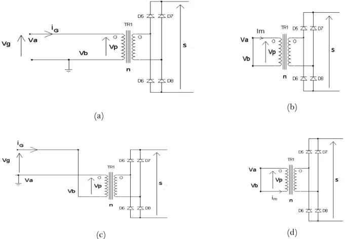
In fact this DC-DC converter alternates between four phases in order to perform its role. In the first phase (Figure 2.8-a) Q1 and Q4 are closed, so the current passes through the first wind and transfers the energy to the second wind, then phase two (Figure 2.8-b) begins by using Q1 and D3 for the HF transformer demagnetization only. After that phase three (Figure 2.8-c) begins by closing Q2 and Q3 so that the current will pass in the reverse path of phase 1 and this will be the negative part of the square signal finally the fourth phase (Figure 2.8-d) will be the demagnetization of the HF transformer by closing Q2 and D4:
Phase 1: (Q1, Q4) closed: from t=0 to t=φT0
Abbass ZEIN EDDINE Page 33
Phase 3: (Q2, Q3) closed: from t=T0 to t= (1+φ) T0
Phase 4: (Q2, D4) closed: from t= (1+φ) T0 to t=2T0
where = /2 and T the period
(a) (b)
(c) (d)
Figure 2.8: Four phases of the DC-DC converter operation: (a) phase 1; (b) phase 2; (c) phase 3; (d) phase 4
The average output voltage S, the ripple inductance current ∆ and the ripple output voltage ∆ are given by equation 2.1 to equation 2.3, where T0 is the switching period and T is the
period of signals and . The output voltage is controlled through the duty cycle φ.
= . = . . ℎ 0 < < 1 (2.1) ∆ = − = . . . . (2.2)
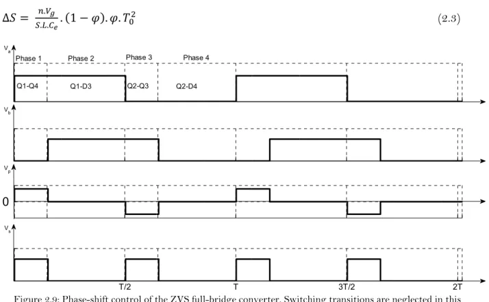
Abbass ZEIN EDDINE Page 34 ∆ = . .. . 1 − . . (2.3)
Figure 2.9: Phase-shift control of the ZVS full-bridge converter. Switching transitions are neglected in this figure.
Figure 2.9 shows the voltages and , during the 4 phases in addition to the primary voltage of the transformer wind and the output voltage S is equal to the absolute value of .
2.3.2 State space model
GREAH laboratory has developed and validated the model of the ZVS full bridge isolated Buck converter in addition to the model of coupling for several DC-DC converters (Guérin et al. 2011), (Mboup et al. 2008) and (Yang et al. 2011) . This model was used to generate simulated data in order to validate and test the proposed FDI methods, before testing on real data.
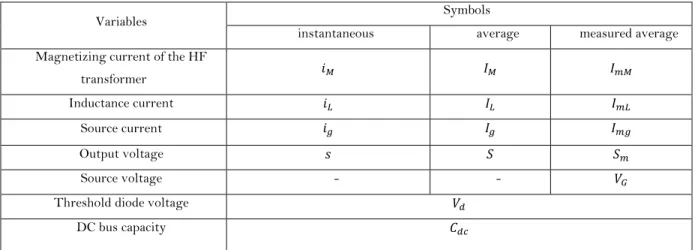
The authors in (Mboup et al. 2008) and (Yang et al. 2011) have developed an average state space model that depends on the duty cycle value φ(t) which is modified by the phase shift between and voltages (Figure 2.7). The main variables are defined in Table 1.
0
T/2 T 3T/2 2T
Phase 1 Phase 2 Phase 3 Phase 4
Q1-Q4 Q1-D3 Q2-Q3 Q2-D4 Vb V p V s V a
Abbass ZEIN EDDINE Page 35
Variables Symbols
instantaneous average measured average Magnetizing current of the HF
transformer Inductance current
Source current Output voltage
Source voltage - -
Threshold diode voltage DC bus capacity
Table 1: Main variables for the DC-DC converter state space model.
Let = , , be the state vector, = , be the input vector and = , , be the output vector. Each one of the four phases is modeled using simple methods as Kirchhoff's circuit laws.
The source voltage ( ) is connected during the phases 1 and 3, so = + . Thus the instantaneous currents and voltage satisfy the following equations:
= − − + (2.4)
= − − − + − (2.5)
= − (2.6) where = , = + and equation 2.4, holds for the phases 1 with ε=+1 and 3 with ε=-1.
Abbass ZEIN EDDINE Page 36 The source voltage ( is disconnected during the phases 2 and 4 which correspond to the transformer demagnetization, thus = 0. Thus the instantaneous currents and voltage satisfy the following equations:
= − − (2.7) = − − − (2.8) = − (2.9) Equation 2.7 holds for phases 2 with ε=+1 and 4 with ε=-1.
The matrices of the state space model for each phase are given as follow: 1. Phase 1: = − 2 + − 2 + 0 − 2 + − + + 2 + −1 0 1 − 1 = 1 0 −2 0 0 , = 10 1 00 0 0 1 2. Phase 2: = − + 0 0 0 − −1 0 1 − 1
Abbass ZEIN EDDINE Page 37 = 0 − 1 0 −2 0 0 , = 0 0 00 1 0 0 0 1 3. Phase 3: = − 2 + 2 + 0 − 2 + − + + 2 + −1 0 1 − 1 = − 1 0 −2 0 0 , = 10 1 00 0 0 1 4. Phase 4: = − + 0 0 0 − −1 0 1 − 1 = 0 1 0 −2 0 0 , = 0 0 00 1 0 0 0 1
From these four phases the average model is generated according to the equations 2.10 and 2.11. These equations stand for the state space model of one DC-DC converter connecting the energy source to the load.
Abbass ZEIN EDDINE Page 38 = φ(t)). + φ(t)).
= φ(t)). + (2.10) Where w(t) represents the measurement error vector. And:
= + 1 − + + 1 −
= + 1 − + + 1 −
= + 1 − + + 1 − (2.11) The matrices A , B and C are given by (2.12):
= + + 0 0 − 2 + − + + 2 + −1 0 1 − 1 = 0. −0 0 0 , = 0 1. 00 0 0 1 (2.12)
, , and are respectively the primary resistance, the secondary resistance, the magnetizing inductance of the HF transformer (TR1) and the MOSFET transistors (Q1,Q2,Q3,Q4) channel resistance. , , and are respectively the coil inductance, the coil
resistance, the capacity and the resistance of the Buck converter. n is the ratio of the HF transformer. is the load.
Subsequently, the multi-converter model (of p converters) is developed by introducing the state vector X = , … , , , the control vector U = , … , and the output vector Y = , … , , where S is the output voltage on the DC bus and p is the number of the coupled converters. By neglecting: the threshold voltage of the diodes ( ), the resistances
Abbass ZEIN EDDINE Page 39 and of primary and secondary coils of the HF transformer, and the resistance of the MOSFETs. The following equation can be derived for every converter i:
+ = . − Then = . − − (2.13) And . = + +…+ − Then = + +… + − (2.14)
The state space matrices , and are defined as (2.15):
= − 0 0 − 0 ⋯ 0 ⋯ 0 1 0 1 0 ⋯ ⋮ 0 ⋯ ⋱⋱ ⋯ 0 1 ⋮ ⋮ 0 0 1 1 01 ⋯⋯ − 1 1 1 . = ⋯ 0 0 0 ⋮ ⋮ ⋯ ⋮⋱ 0 0 ⋯ 0 0 ⋯ ⋯ 0 = . (2.15)
Abbass ZEIN EDDINE Page 40 where CEQ and REQ represent the equivalent capacitance and resistance in the whole system.
The model developed in (Yang et al. 2011) represents multi DC-DC converters coupled together on the DC-bus in order to satisfy the load. This model takes into consideration a Buck-Boost converter that uses the batteries as source (discharge) or storage (charge), which is not our interest. Thus we developed the model in 2.15, which represent a system of identical multiple DC-DC converters.
2.4 Reliability in static converters
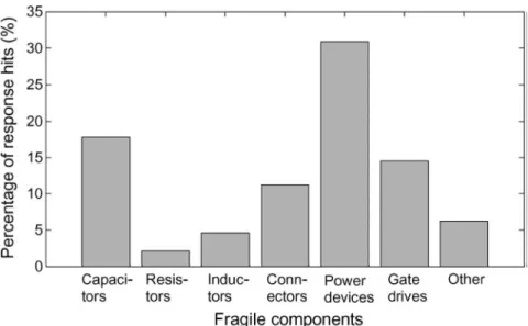
Static converters are faulty-prone and they are often subjected to unexpected failure of components which degrade the performance. In static converters the power semiconductor devices (MOSFET, gate drivers, diodes) are the components with the lowest reliability (Griffin et al. 2002) followed by the other types of components (capacitors, inductors, resistors …). Figure 2.10 shows the percentage of the components reliability based on industry survey of components reliability (Griffin et al. 2002). Another survey (Huang and Flett 2007) states that power semiconductors, are the most vulnerable components, since 40% of all failures start from these elements. This study considers the reliability of transistors (MOSFETs), diodes, and inductors which in total represent about 45-50 % of the system failure causes.
Abbass ZEIN EDDINE Page 41 The failures that may affect MOSFET transistors, inductors, capacitors and diodes will be briefly introduced in the next section.
2.4.1 MOSFET faults
Faults of MOSFET transistors are decomposed into several categories. Some of them are detected at the stage of constructing the circuit or before that. Such as manufacturing faults, these faults are rare to happen because most of the equipment are tested (using soak testing) before using, or they appear at the first hours of converter use. Sometimes external causes may damage MOSFET transistors, such as applying a high-voltage static electricity. Some components such as resistors may suffer from aging which leads to changing their values and MOSFET transistors in the same circuits may start to operate outside their normal parameters. But usually when MOSFET transistors fail, one of three things happens:
(i) Short-circuit (its channel resistance becomes very low or zero). (ii) Open-circuit (its channel resistance become very high of infinity) (iii) Leak (slightly low channel resistance).
The most common failures are the open and short-circuit faults (Ismail et al. 2006), (Chow and Willsky 1984). Those failures may occur due to external or internal events such as : incorrect gate voltage, lifting of bonding wire due to thermal cycling, driver failure, rupture of the switch which can be a consequence of a short-circuit fault or electrical over stress voltage or current.
2.4.2 Inductor faults
The insulation material covering the inductor wire may break down and causes a short-circuit which may increase the current to flow and overheating occurs. If the magnetic core does not seat correctly in the inductor, it will alter the inductance and leads to overheat due to over current. In addition a broken conductor in an inductor that is caused by mechanical collision, overheating or vibrations, will mean that the inductor does not perform as expected.
The causes of inductor failures may be due to three factors (Denson 1992):
1- Design failures: before the construction of the inductor, failures can result from fundamental design flaws, inappropriate material specification, improper test specification, or insufficient installation guidelines.
Abbass ZEIN EDDINE Page 42 2- Manufacturer failures: during the construction of the inductor, several mistakes can appear, such as using wrong materials, improper manufacturing process, poor workmanship, incorrect assembly or improper handling (packaging and transportation)
3- Installation failures: during the installation level, failures may result due to the poor installation workmanship, inappropriate connections, wrong or unstable handling, or non-conformance with installation specifications.
2.4.3 Diode faults:
Diodes are used in most of the static converter circuits especially in the rectifiers (as the secondary circuit with four diodes). The main faults that may affect diodes are the short-circuit faults where diodes can be easily damaged by high voltage or direct current which leads to a low or zero resistance. Also the open-circuit fault when the resistance of the diode becomes very high in both reverse and forward directions. In addition a leakage fault appears when the reverse resistance becomes lower than the expected infinity.
2.4.4 Capacitor faults:
Capacitors are used as filters and power suppliers in some cases, and mainly they suffer from three faults:
(i) Open circuit such that its resistance goes to infinity. (ii) Short circuit, i.e. zero ohm resistance.
(iii) Leak capacitance, a partial short circuit where the dielectric gradually losses its insulating qualities under the stress of the applied voltage thus lowering its resistance.
Mainly the faults of capacitor vary its resistance thus this component is monitored by putting resistance under surveillance.
2.5 Considered faults
As presented in the previous section, numerous electrical failures are due short-circuit faults, open-circuit faults or leakages. Short-circuit faults in most cases cause an over-current that are readily detected by the standard protection systems. A short circuit fault can appear and can become an open circuit fault 100ms after due to the thermal effect (the component looks like a fuse!). It is difficult to predict and model this phenomenon. However, open-circuit faults do not
Abbass ZEIN EDDINE Page 43 trigger standard protection systems because the voltage and current during these faults often do not exceed the threshold limits for the standard protection systems. Alternatively, they cause system malfunction or performance degradation. Therefore, those faults become critical to static converters (kamel et al. 2015). Thus, in our study we have considered the open circuit faults for the main components of the DC-DC converter:
(i) MOSFET transistors open-circuit fault (fault 1) (ii) Diode open-circuit fault (fault 2)
(iii) Coil open-circuit fault (fault 3)
The occurrence of each fault will lead to a modification in one or more phases of the DC-DC converter operation, which will also lead to a change in the average model. In order to test the proposed algorithms on simulated data before using real data, the average model of some specific cases is generated for each fault type as follow: MOSFET transistor open-circuit, diode open-circuit and coil open-circuit (Figure 2.7). Such models will be used to emulate the behavior of the DC-DC converters in faulty conditions.
2.5.1 MOSFET transistor (Q1) open-circuit fault model (fault 1)
Q1 open-circuit fault will affect the first two running phases such that =0 and =0, since in fault free system Q1 is ON in both phases 1 and 2 whereas its actually OFF (open) in phases 3 and 4. So no current can flow in the primary circuit during the first two running phases. This means that = 0, = − − − and = − during phase 1 and 2. The average model which corresponds to this fault is given by equation 2.16:
= − +2 + + +2 2 + 2 − 2 2 + − 2 + 2+ . + 2 + −1 0 1 − 1 = − −1/ 0 0 , = 0 0 1 0 0 0 (2.16)
Abbass ZEIN EDDINE Page 44
2.5.2 Diode (D8) open-circuit fault model (fault 2)
In this case only running phase one should be considered and is the only affected parameter. The only difference between fault 2 average model and fault free average model occurs in matrix with the row that corresponds to and the column that corresponds to
. The average model which corresponds to this fault is given by equation 2.17:
= − 0 0 − − − 0 − = 0 −2/0 0 0 , = . 0 0 1 0 0 0 1 (2.17)
2.5.3 Coil (L) open-circuit fault model (fault 3)
Coil (L) open-circuit fault influences the four running phases. In this case the secondary circuit will be open-circuit and becomes equal to zero, thus = . In addition the primary circuit variables ( , , are no longer related with the secondary circuit variables ( , S).All the columns and rows related to in and are affected. The average model which corresponds to this fault is given by equation 2.18:
= − + + 0 0 0 0 0 0 0 − 1 = 0 00 0 0 0 , = . 0 0 1 0 0 0 1 (2.18)
2.6 Conclusion
In this chapter, an overview of DC-DC converters is presented. Then the operation and the state space model of the ZVS full bridge isolated Buck converter are detailed. A general idea of the system of multi-sources of energy is given. Moreover, the reliability of the static converters
Abbass ZEIN EDDINE Page 45 is discussed and the considered faults with their state space models are detailed. The next chapter will present a literature review about fault detection and isolation methods in general and their use in DC-DC converters in special.
Abbass ZEIN EDDINE Page 47
Chapter 3
F
AULT
D
ETECTION AND
I
SOLATION
(FDI)
METHODS
3.1 Introduction
Fault detection and Isolation (FDI) methods are found to empower machines from monitoring themselves to improve their performance with the minimal human interference. Obviously there are two parts, firstly the detection part, secondly the isolation part. Fault detection is the determination of the appearance or disappearance of the fault i.e. if the measured observations notifies about a coming fault or not. While the second task (isolation) shows the type and the location of the detected fault. This chapter lists some of the FDI methods and their use in power electronics FDI domain; in addition it details the Bayesian belief network method.
3.2 Fault detection and isolation
To perform the two tasks of fault detection and isolation, two modes can be followed, first by human, i.e. manually by monitoring the output of a given system with the help of some experts to detect faults as well as diagnosis. This way of treating such problems are no more efficient due to the complexity of modern systems plus the distributed system models that are widely used today, in addition some processes are dangerous to monitor and control as in the case of chemical processes.
Another technique to achieve fault detection and isolation is to automate the monitoring and diagnosis, by mandating the jobs to the machine. This is done by Fault Detection and Isolation (FDI) methods which excel the previous mode not only in efficiency but also in time detection. Systematic methods improve the performance. FDI schemes can be classified as hardware (physical) methods and software (analytical) methods as shown in Figure 3.1. In addition,
Abbass ZEIN EDDINE Page 48 analytical methods can be categorized by several ways depending on the features of categorization. For example methods can be classified into two categories: statistical or non-statistical. Moreover, the main components in diagnosis classifiers are: (i) the type of knowledge and (ii) the type of diagnosis search strategy. Diagnosis search strategy is usually a very strong function of the knowledge representation scheme which in turn is largely influenced by the kind of a priori knowledge available. Hence, the type of a priori knowledge used is the most important distinguishing feature in diagnosis systems (Venkatasubramanian et al. 2003).
The main a priori knowledge needed for fault diagnosis is denoted by the set of failures and the relation between the observations and those failures. This knowledge can be acquired by (i) gathering them from historical (knowledge) data in form of table; (ii) developing them from a deep understanding of causal relationships between process variables, inputs and outputs. Such methods are recognized as model-based methods. Thus, the analytical FDI methods are classified as model-based methods or knowledge-based methods (Figure 3.1).
Figure 3.1: Classification of FDI methods (Patton et al. 1989)
3.2.1 Hardware (physical) FDI
Hardware FDI employs repeated hardware elements (actuators, components or sensors) (Abid 2010). An indication of a fault can be obtained if the behaviors of the process components are different from the redundant ones. Hardware FDI can also be implemented by adding
Abbass ZEIN EDDINE Page 49 additional sensors which are especially included for the purpose of monitoring and a fault can be located by comparison of measured signals with predefined thresholds. Hardware FDI can be straightforward and is widely used in many safety-critical applications such as aircraft systems and nuclear plants (Abid 2010). The main problem of this approach is the extra cost, space and weight (Kinnaert 2003). Besides, the additional hardware itself will reduce the reliability of the system.
3.2.2 Software (analytical) FDI
Analytical redundancy concept is the opposite of physical redundancy. In physical redundancy, hardware (sensors) are duplicated to provide several measurements for the variables and parameters of concern. While in analytical redundancy the process is either modeled using its physical and mathematical equations, or by learning the process dynamics via historical data. The first are the model-based methods that depend on the mathematical and physical equations of the system, and the latter are the knowledge-based methods that are based on historical data previously collected from the real system or by simulation.
3.2.2.1 Model-based FDI methods
Model-based methods require a model of the process (Figure 3.2). The system is duplicated in a software manner according to its mathematical and physical equations, and then the values for parameters of interest are extracted. Then residuals are generated by the comparison of measurements and expected values. These residuals are analyzed in order to detect and diagnose faults. In average the value of the residuals in the fault free case is equal to zero, since the estimated value and the real measurements are equal. While in the faulty case the residuals will deviate from zero and give an indication of fault occurrence. The three main ways to generate residuals are parameter estimation, parity relations and observers (Garcia et al. 1996).
Parameter estimation: For parameter estimation, the residuals are the difference between
the nominal model parameters and the estimated model parameters. Deviation in the model parameters serve as the basis for detecting and isolating faults (Isermann 1984), (Ding and Guo 1996).
Parity relations: This method checks the consistency of the mathematical equations of the
Abbass ZEIN EDDINE Page 50 transformation, with the transformed residuals used for detecting and isolating faults (Mironovskii 1980), (Aronson et al. 2005).
Observers: The observer-based method reconstructs the output of the system from the
measurements or a subset of the measurements with the aid of observers. The difference between the measured outputs and the estimated outputs is used as the vector of residuals (Frank 1990), (Mironovskii 1979).
Figure 3.2: Basic concept of model-based FDI techniques (Yang et al. 2009).
3.2.2.2 Knowledge-based FDI methods
This type of methods uses the history of data collected from the process. Most of the processes are usually under usage which means that they have historical data that may be used in order to detect and isolate faults. Mostly, those types of methods are used for complex systems that are difficult to represent by a given mathematical or physical model (transfer functions, state space …). Furthermore in practice it is almost impossible to obtain a model that exactly matches the process behavior (Mohamed et al. 2002), therefore it is necessary to have alternative approach such as knowledge-based methods.
Historical data can be represented in two different forms; it may be as a human knowledge understanding and describing the studied process (expert), or as tables that collect data representing the system. Some of the well-known knowledge-based methods are the expert systems, Artificial Neural Network (ANN), and the Bayesian Belief Network (BBN).
Expert systems: Human mental process is internal, and it is too complicated to be
represented as an algorithm. On the other hand, most experts are able to express their knowledge in the form of rules for problem solving. Rules are the most commonly used type of knowledge representation and are often defined as an If-Then structure that relates given information or facts:
(IF <antecedent> THEN <consequent> )
Location of faults Residuals
Measured states
System Residual generation parity function or observer
Decision module
Abbass ZEIN EDDINE Page 51 Expert system is a system that uses human knowledge captured (in the form of rules) in a computer to solve problems that ordinarily require human expertise (Angeli 2010).
In fault detection and diagnosis expert systems, rules should represent the fault type if a given set of symptoms is observed; moreover the knowledge base must contain all the possible faults in addition to their symptoms. The user interface will present the possible symptom to the user, who in turn clicks the specific symptoms in order to start a searching process (Hecht-Nielsen 1989)(by the inference engine) in order to isolate the fault.
Artificial Neural Network (ANN): Artificial Neural Network(ANN) is one of the
non-probabilistic predictive algorithms, it was defined by Dr. Robert Hecht-Nielsen - which is an inventor of one of the first Neuro-computers – as "...a computing system made up of a number of simple, highly interconnected processing elements, which process information by their dynamic state response to external inputs” (Rahman 2010).
Neural networks are often used for modeling complex relationships between inputs and outputs or to find patterns in data. ANNs consists of three main layers: input layer (single layer), hidden layer (may be multi layers) and output layer (single layer). These layers are connected via arcs that are associated by weights.
Neural networks are extensively used in fault detection and diagnosis domain. Mainly neural network applications in this domain are recapitulated in three types. NNs are used to discriminate a variety of fault patterns from normal operating conditions. Moreover neural networks are used as classifiers to isolate faults from the residuals, and finally a neural process model can be employed to generate residuals plus another network used for fault isolation (Rahman 2010).
Bayesian Belief Network (BBN): Bayesian belief network is a probabilistic graphical model
that represents a set of random variables and their conditional dependencies via a Directed Acyclic Graph (DAG). A detailed presentation will be provided in section 3.4.
3.3 Fault detection and isolation in DC-DC converters
Generally a short-circuit fault requires quick detection and isolation in order to avoid the damage of the complementary device. This is done using hardware circuits. On the other hand, open-circuit faults are not immediately fatal and can be tolerated by the power converter for
Abbass ZEIN EDDINE Page 52 some time. Therefore, open-circuit faults can typically be detected using analytical methods which normally take a few tens of milliseconds to detect and isolate the fault.
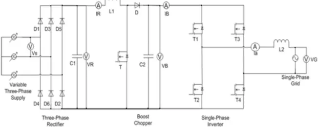
Hardware detection methods are widely used due to their efficiency and speed in detection and isolation, but their main drawback results from redundancy which leads to an increase in the cost. Hardware detection techniques are mostly based on the desaturation method, current mirror (Huang and Flett 2007), and gate voltage sensing methods (Rodrigues et al. 2007). Most of the work found in the literature using such techniques focus on power semi-conductors, and are normally implemented along with the gate drive circuit. This gate drive and its capability for fault detection and over current protection is often called “active drive” or “smart gate drive” (Vinnikov et al. 2009), (Cordeiro et al. 2014) and (Zheng and Li 2015).
Figure 3.3: Grid-connected power converter (Kalman 2015).
Analytical FDI methods have variable detection time periods, which typically range between 10ms and 60ms. So they are slower in detection and isolation than the hardware methods. But they represent an active research topic for FDI in power converters, due to the fact that there is no need for hardware redundancy and additional costs. Most of the work found in the literature tackles the problem of fault detection and isolation in single DC-DC converter, while rare are the papers that expose to the problem of fault detection and isolation in multi DC-DC converters. In (Kamel et al. 2016) the authors considered a system of three consecutive converters (Figure 3.3), the uncontrolled three-phase rectifier, the boost chopper and the single-phase inverter. Three FDI methods are discussed one for each converter. First, for the rectifier, the diodes open-circuit faults are studied, in addition, to the unbalanced input voltage