HAL Id: tel-02145121
https://tel.archives-ouvertes.fr/tel-02145121
Submitted on 1 Jun 2019
HAL is a multi-disciplinary open access
archive for the deposit and dissemination of sci-entific research documents, whether they are pub-lished or not. The documents may come from teaching and research institutions in France or abroad, or from public or private research centers.
L’archive ouverte pluridisciplinaire HAL, est destinée au dépôt et à la diffusion de documents scientifiques de niveau recherche, publiés ou non, émanant des établissements d’enseignement et de recherche français ou étrangers, des laboratoires publics ou privés.
Analyse multifractale de mesures faiblement Gibbs
aléatoires et de leurs inverses
Zhihui Yuan
To cite this version:
Zhihui Yuan. Analyse multifractale de mesures faiblement Gibbs aléatoires et de leurs inverses. Géométrie algébrique [math.AG]. Université Sorbonne Paris Cité, 2015. Français. �NNT : 2015US-PCD098�. �tel-02145121�
No
d’ordre:
THÈSE
pour obtenir le grade de
DOCTEUR EN SCIENCES DE L’UNIVERSITÉ PARIS-NORD XIII
Discipline: Mathématiques
présentée et soutenue publiquement par
Zhihui YUAN
le 17 Décembre 2015
Analyse multifractale de mesures faiblement
Gibbs aléatoires et de leurs inverses
Directeur de thèse:
M. Julien BARRAL
La Commission d’examen:
M. Julien Barral Université Paris 13 M. Henry De Thelin Université Paris 13
M. Aihua Fan Université de Picardie Jules Verne M. Volker Mayer Université Lille 1
M. Jacques Peyrière Université Paris-Sud XI
M. Stéphane Seuret Université Paris Est Créteil - Val de Marne
Rapporteurs:
M. Wen Huang University of Scince and Technology of China M. Mariusz Urbanski University of North Texas
LAGA
Institut Galilée
Université Paris 13
99, avenue Jean-Baptiste Clément
93430 - Villetaneuse
Résumé
Nous montrons la validité du formalisme multifractal pour les mesures aléatoires fai-blement Gibbs portées par l’ attracteur associé à une dynamique aléatoire C1 codée par un sous-shift de type fini aléatoire, et expansive en moyenne. Nous établissons également des loi de type0-∞ pour les mesures de Hausdorff et de packing généralisées des ensembles de niveau de la dimension locale, et calculons les dimensions de Hausdorff et de packing des ensembles de points en lesquels la dimension inférieure locale et la dimension supé-rieure locale sont prescrites. Lorsque l’attracteur est un ensemble de Cantor de mesure de Lebesgue nulle, nous montrons la validité du formalisme multifractal pour les mesures discrètes obtenues comme inverses de ces mesures faiblement Gibbs.
Mots-clefs: Mesures et dimensions de Hausdorff et de packing, formalisme multifractal, formalisme thermodynamique, mesure faiblement Gibbs aléatoires, systèmes dynamiques aléatoires, théorie métrique de l’approximation, mesures inverses.
Multifractal analysis of random weak Gibbs measures and their inverse
Abstract
We establish the validity of the multifractal formalism for random weak Gibbs mea-sures supported on the attractor associated with a C1random dynamics coded by a random subshift of finite type, and expanding in the mean. We also prove a0-∞ law for the gen-eralized Hausdorff and packing measures of the level sets of the local dimension, and we compute the Hausdorff and packing dimensions of the sets of points at which the lower and upper local dimensions are prescribed. In the case that the attractor is a Cantor set of zero Lebesgue measure, we prove the validity of the multifractal formalism for the discrete measures obtained as inverse of these weak Gibbs measures.
Keywords : Hausdorff and packing measures and dimensions, multifractal formalism, thermodynamic formalism, random weak Gibbs measure, random dynamical systems, met-ric approximation theory, inverse measures.
Remerciements (Acknowledgement)
I would like to express my gratitude to all those who helped me during the writing of this thesis.
My deepest gratitude goes first and foremost to Professor Julien Barral, my supervisor, for his patience, enthusiasm, wide knowledge, constant encouragement and guidance. His guidance helped me in all the time of research and writing of this thesis. Without his help, this thesis could not appear.
I would like to express my heartfelt gratitude to Professor Zhiying Wen, who led me into this field and helped me a lot in my study and research.
I gratefully acknowledge the funding from China Scholarship Council, who supported me for my study and research in France from 2011 to 2013. Also, I need to thank Professor Jiayan Yao and Dr. Yanhui Qu, who helped me a lot for my preparation to come France.
I am indebted to LAGA and the group of dynamical system and ergodic theory. I am thankful to Professor Dejun Feng. He and his department supported me to go Hong Kong twice. They gave me the chance to know their works and to see my supervisor Professor Barral there.
I would like to thank Professor Wen Huang and Mariusz Urbanski. They read this thesis carefully, gave their reports and proposed some good advices. I would also like to thank Professor Julien Barral, Henry De Thelin, Aihua Fan, Volker Mayer, Jacques Peyrière and Stéphane Seuret for their consent to being my dissertation committee.
I also thank my friends who helped me, both in China and in France.
I would like to thank my parents who have always been helping me out of dif-ficulties and supporting without a word of complain. I would like to express my gratitude to my wife, Ying Yang. She took care of our family and supported me heart and soul. She was always there cheering me up and stood by me for better and worse. I also need to refer that the happiness from my daughter gives me lots of energy.
Contents
1 Introduction 1
1.1 Weak Gibbs measures on random subshifts . . . 3
1.2 A model of random dynamical attractor . . . 7
1.3 Multifractal formalism . . . 9
1.4 Multifractal analysis of the random weak Gibbs measures . . . 13
1.5 Multifractal analysis of the inverse of random weak Gibbs measures . 16 1.6 Concrete examples of random attractors . . . 22
2 Basic properties of random weak Gibbs measures 25 3 Basic properties of random Gibbs measures 31 4 Proof of Bowen’s formula 34 5 Approximation of (Φ, Ψ) and related properties 37 5.1 Approximation of (Φ, Ψ) by random Hölder potentials . . . 37
5.2 Approximation of (T, T∗) by (Ti, Ti∗) . . . 38
5.3 Explanation of some variational formulas . . . 40
5.4 Simultaneous control for random Gibbs measures associated with (Φi, Ψi) . . . 42
6 Multifractal of random weak Gibbs measures 49 6.1 Lower bound for τµω and upper bound for τµ∗ω . . . 49
6.2 Lower bound for the Hausdorff spectrum . . . 51
6.3 Proofs of theorems 1.11(3), (4) and (5) . . . 61
7 Multifractal analysis of the inverse measures 66
7.1 Some notations . . . 66
7.2 An explicit writing of the inverse measure νω, and preliminary esti-mates for the mass of atoms . . . 67
7.3 Pointwise behavior of νω and an upper bound for the lower Hausdorff spectrum without using of multifractal formalism . . . 70
7.4 Upper bound for the lower Hausdorff spectrum . . . 75
7.5 First lower bound for the lower Hausdorff spectrum . . . 78
7.6 Some preparation to the conditioned ubiquity theorem . . . 81
7.7 Conditioned ubiquity . . . 86
7.8 Conclusion on the lower bound for the lower Hausdorff spectrum . . . 99
7.9 Hausdorff dimensions of the level sets E(νω, d) and E(νω, d) . . . 101
Bibliography 107
Chapter 1
Introduction
Weak Gibbs measures are conformal probability measures obtained as eigenvec-tors of Ruelle-Perron-Frobenius operaeigenvec-tors associated with continuous potentials on topological dynamical systems. When the system (X, f ) has nice enough geometric properties, for instance in the case of a conformal repeller, these measures provide natural, and now standard examples of measures obeying the multifractal formalism: their Hausdorff spectrum and Lq-spectrum form a Legendre pair.
Specifically, for such a measure µ on (X, f ), the (lower) Lq-spectrum τ
µ : R → R∪ {−∞} is defined by τµ(q) = lim inf r→0 log sup{Pi(µ(Bi))q} log(r) , (1.1)
where the supremum is taken over all families of disjoint closed balls Bi of radius r
with centers in supp(µ); the lower Hausdorff spectrum of µ is defined by
d∈ R 7→ dimH E(µ, d),
where dimH stands for the Hausdorff spectrum, E(µ, d) is the level set of level d of
the lower local dimension dimloc(µ, x) = lim inf r→0+
log(µ(B(x, r))) log(r) , i.e. E(µ, d) ={x ∈ supp(µ) : dimloc(µ, x) = d} ,
and we have the duality relation
dimHE(µ, d) = τµ∗(d) := infq
∈Rdq− τµ(q), ∀d ∈ R,
a negative dimension meaning that the set is empty. In fact, due to the super and submultiplicativity properties associated with µ, the same equality holds if we replace the lim inf by a lim sup or a limit in the definition of the local dimension.
2
The rigorous study of these measures started with the Gibbs measures case, which corresponds to Hölder continuous potentials, or continuous potentials pos-sessing the so-called bounded distorsions property, and in particular on the so-called “cookie-cutter” Cantor sets associated with a C1+α expanding map f on the line
[19, 71] (see [68] for an extended discussion of dimension theory and multifractal analysis for hyperbolic conformal dynamical systems). This followed seminal works by physicists of turbulence and statistical mechanics pointing the accuracy of mul-tifractals to statistically and geometrically describe the local behavior of functions and measures [33, 36]. In the case of Gibbs measures, the Lq-spectrum of the Gibbs
measure is differentiable, and analytic if the potential φ is Hölder continuous; it is the unique solution t of the equation P (qφ + t logkDfk) = 0, where P (·) stands for the topological pressure. The general case of continuous potentials was solved later in [26, 29, 42, 63], with the same formula for the Lq-spectrum. These progress then led
to the multifractal analysis of Bernoulli convolutions associated with Pisot numbers [28, 30]. Thermodynamic formalism and large deviations are central tool in these studies. It is worth mentioning that simultaneously another family of multifractal measures has been studied intensively, namely the random measures possessing scale invariance in multiplicative chaos theory (see [55, 56, 57, 41, 5, 72, 3]).
It turns out that Gibbs measures on cookie-cutter sets naturally generate a class of discrete measures obtained as their inverse (see Definition 1.12), for which the validity of the multifractal formalism was established in [11], after a partial study in [58, 73, 74]. Given such a Gibbs measure µ, the Lq-spectrum of its right continuous
inverse measure ν is given by τν(q) = min(0,−τµ−1(q)); in [11], an essential new
ingredient is needed, namely conditioned ubiquity [8], which combines ergodic theory and metric approximation theory.
In the context of random dynamical systems, the multifractal analysis of random Gibbs measures (to be defined below) associated with random Hölder continuous po-tentials on attractors of random C1+α expanding (or expanding in the mean) random
conformal dynamics encoded by random subshifs of finite type has been studied in [45], [31] and [61]. These works, as well as the dimension theory of attractors of random dynamics [15, 45, 46, 61], are based on the thermodynamic formalism for random transforms [14, 15, 20, 21, 22, 35, 43, 44, 49, 61]. The multifractal analysis of random weak Gibbs measures is also implicitly considered in [31] (which deals with the multifractal analysis of Birkhoff averages), but the fibers are deterministic, and the techniques developed there seems difficult to adapt in a simple way in the case of random subshifts.
In this thesis we consider, on a base probability space (Ω,F, P, σ), random weak Gibbs measures on some class of attractors included in [0, 1] and associated with C1 random dynamics semi-conjugate (up to countably many points), or conjugate,
to a random subshift of finite type, and show that these measures and their inverse obey the multifractal formalism. Compared to the above mentioned works, apart the source of new difficulties coming from the relaxation of the regularity
proper-CHAPTER 1. INTRODUCTION 3
ties of the potentials, our assumptions provide a slightly more general process of construction of the random Cantor set in terms of the distribution of the random family of intervals used to refine the construction at a given step: it can contain contiguous intervals (i.e. without gap in between, and even no gap) with positive probability; thus, it covers the natural families of Cantor sets one can obtain by picking at random a fiber in a Bedford-McMullen carpet. As a consequence, the expression and study of the inverse measure are more involved than in the standard and deterministic situation considered in [8]. Moreover, we succeed in developing ubiquity theory in this random context without assuming any mixing properties on the base space (Ω,F, P, σ). This substantially improves the approach developed in [7] to get ubiquity results associated with the special class of random Gibbs mea-sures obtained as random Riesz products, for which the product structure of (Ω, P) plays an essential role.
Before stating our main results, we introduce some background about random dynamical systems and thermodynamic formalism.
1.1 Weak Gibbs measures on random subshifts
Now let us introduce the concepts of random subshifts and associated topological pressure of random continuous potentials. They have been studied by many authors [14, 15, 34, 44, 43, 49, 61].
Assume that (Ω,F, P) is a complete probability space and σ is a P-preserving invertible ergodic map. In fact, assuming that P is σ-invariant and it has an ergodic decomposition is enough (this holds if, for example, F is a countably generated (separable) σ-algebra). Also, we do not really need to assume the map σ to be invertible; assuming that σΩ = Ω or that σnΩ is measurable for all n ≥ 0 makes
it possible to construct a Rokhlin natural extension which preserves the ergodicity and mixing (see [79, theorem 1.5] or [70, section 2.7]).
Let‹Z+ ={1, 2, · · · }∪{∞} be the one-point compactification of Z+ ={1, 2, · · · }.
Let Γ :=Z‹+׋Z+× · · · with the metric on Γ given by d(v, v′) =X i∈N exp(−i) 1 vi − 1 v′ i .
where v = v0v1· · · vi· · · , v′ = v0′v1′ · · · v′i· · · and we set ∞1 = 0.
Let l be a Z+ valued random variable such that
ˆl:= Z log(l) dP < ∞ and P({ω ∈ Ω, l(ω) ≥ 2}) > 0. Here, l(ω) will define the number of types for a fixed ω.
Let A = {A(ω) = (Ar,s(ω)) : ω ∈ Ω} be a random transition matrix such
4 Weak Gibbs measures on random subshifts
ω 7→ Ar,s(ω) is measurable for all (r, s)∈ ‹Z+׋Z+ and each A(ω) has at least one
non-zero entry in each row and each column. Let
Σω ={v = v0v1· · · ; 1 ≤ vk≤ l(σk(ω)) and Avk,vk+1(σ
k(ω)) = 1 f or k∈ N},
and Fω : Σω → Σσω be the left shift (Fωv)i = vi+1 for any v = v0v1· · · ∈ Σω.
Define ΣΩ = {(ω, v) : ω ∈ Ω, v ∈ Σω} and the map Π : ΣΩ → Ω as Π(ω, v) = ω.
Define the map F : ΣΩ → ΣΩ as F ((ω, v)) = (σω, Fωv). The corresponding family
˜
F = {Fω : ω ∈ Ω} is called a random subshift.
We assume that the random subshift defined above is topologically mixing, i.e. there exists a N-valued random variable M = M (ω) < +∞ on (Ω, F, P) such that for P-almost every ω,
A(ω)A(σω)· · · A(σM−1ω) is positive.
It is not hard to see that this implies that one can choose M = M (ω) such that for P-almost every ω,
A(σ−Mω)A(σ−M+1ω) . . . A(σ−1ω)
and A(ω)A(σω)· · · A(σM−1ω) are positive. (1.2) Define Σω,n = ® v = v0v1· · · vn−1: 1≤ vk ≤ l(σ k(ω)) for 0 ≤ k ≤ n − 1, and Avk,vk+1 = 1 for 0≤ k ≤ n − 2. ´ .
By convention we write Σω,0 = ∅. Define Σω,∗ = Sn≥0Σω,n. For v =
v0v1· · · vn−1 ∈ Σω,n, we denote |v| = n. For such v, we define the cylinder [v]ω
as
[v]ω :={w ∈ Σω : wi = vi for i = 0, . . . , n− 1}.
Now let us introduce basic notations. For any word v = v0· · · vr−1vr· · · vm−1 ∈
Σω,m, define v0 to be the first character of v and vm−1 to be the last character of v.
For r ≤ m, define v|r = v0· · · vr−1.
For any 1 ≤ s ≤ l(ω), for any n ≥ M(ω), for any 1 ≤ t ≤ l(σnω), there exists
at least one word v = v(ω, n, s, t)∈ Σσω,n−1 such that svt∈ Σω,n+1. The choice of v may be not unique. For each such v, we denote the word svt by s∗ t.
For any v = v0v1· · · vn−1 ∈ Σω,n and w = w0w1· · · wm−1 ∈ Σσn+kω,m, if k ≥ M (σnω), then v
0v1· · · vn−2vn−1∗ w0w1· · · wm−1∈ Σω,n+k+m−1.
For any v = v0v1· · · vn−1· · · ∈ Σω, define v|n = v0v1· · · vn−1.
For any v = v0v1· · · vr−1vr· · · vn, w = w0w1· · · wr−1wr· · · wn, if for any i, 0 ≤
CHAPTER 1. INTRODUCTION 5
subshift of finite type Random subshift ———– (Ω,F, P, σ) l ( the number of types) constant random variable A = (ai,j) (Transitive matrix) constant matrix random matrix
M (To define the mixing property) constant random variable
v = v0v1. . . vn. . . (Point) 1≤ vi ≤ l Avi,vi+1 = 1 v ∈ Σ 1≤ vi ≤ l(σi(ω)) Avi,vi+1(σ i(ω)) = 1 v ∈ Σω shift operator Σ→ Σ Σω → Σσω
Table 1.1 – The differences between subshift of finite type and random subshift
The differences between subshift of finite type and random subshift of finite type are indicated in Table 1.1.
Using the same notations as in [44, 47, 49], let
PP(ΣΩ) ={ρ, probability measure on ΣΩ : Π∗ρ = ρ◦ Π−1 = P},
and
IP(ΣΩ) = {ρ ∈ PP(ΣΩ) : ρ is F -invariant}.
Any ρ ∈ PP(ΣΩ) on ΣΩ disintegrates in dρ(ω, v) = dρω(v)dP(ω) where the
measures ρω, ω ∈ Ω, are regular conditional probabilities with respect to the
σ-algebra πΩ−1(F), where πΩ is the canonical projection from ΣΩ to Ω. This implies
that for P-almost every ω, for any measurable set R⊂ ΣΩ, ρω(R(ω)) = ρ(R|π−1Ω (F)),
where R(ω) ={x : (ω, v) ∈ R}.
LetR = {Ri} be a finite or countable partition of ΣΩ into measurable sets. Then
for all ω ∈ Ω, R(ω) = {Ri(ω) : Ri(ω) ={x ∈ Σω : (ω, x) ∈ Ri}} is a partition of
Σω.
Given ρ∈ PP(ΣΩ), the conditional entropy ofR given πΩ−1(F) is defined by
Hρ(R|πΩ−1(F)) = − Z X i ρ(Ri|πΩ−1(F)) log(ρ(Ri|π−1Ω (F)))dP = Z Hρω(R(ω))dP(ω)
where Hρω(A) denotes the usual entropy of a partition A.
Now, given a finite or countable partitionQ of ΣΩ, define the fiber entropy of F
or the relative entropy of F with respect to Q as hρ(F,Q) = limn →∞ 1 nHρ(∨ n−1 i=0F−iQ|πΩ−1(F))
6 Weak Gibbs measures on random subshifts
(here ∨ denotes the join of partitions). Then define
hρ(F ) = sup
Q hρ(F,Q),
where the supremum is taken over all finite or countable measurable partitions Q = {Qi} of ΣΩ with finite conditional entropy, that is hρ(F,Q) < +∞. In our
setting, we have hρ(F ) ≤
R
log(l) dP. The number hρ(F ), also denoted h(ρ|P) in the
literature, is the relativized entropy of F given ρ. It is also called the fiber entropy of the bundle random dynamics F .
We say that a measurable function Φ on ΣΩ is in L1ΣΩ(Ω, C(Σ)) if 1. CΦ =: Z ΩkΦ(ω)k∞dP(ω) <∞ (1.3) where kΦ(ω)k∞=: sup v∈Σω |Φ(ω, v)|; (1.4) 2.
varnΦ(ω)→ 0 as n → ∞, P-almost surely (1.5)
where varnΦ(ω) = sup{|Φ(ω, v) − Φ(ω, w)| : vi = wi,∀i < n}.
The topological pressure P (Φ) of Φ is defined by
P (Φ) = sup ρ∈IP(ΣΩ) ß hρ(F ) + Z Φdρ ™ . Now, with Φ∈ L1
ΣΩ(Ω, C(Σ)) is associated the transfer operator L
ω Φ : C0(Σω)→ C0(Σ σω) defined as LωΦh(v) = X Fωw=v exp(Φ(ω, w))h(w), ∀ v ∈ Σσω.
By replacing if necessary Ω by a subset of full probability over which the mappings Φ(σkω,·), k ≥ 0 are all continuous, we have the following result:
Proposition 1.1 [44, 61] For all ω ∈ Ω, there exists λ(ω) > 0 and a probability measure µeω on Σω such that (LωΦ)∗µeσω= λ(ω)µeω.
We call the family {µeω : ω ∈ Ω} a random weak Gibbs measure on {Σω : ω ∈ Ω}
CHAPTER 1. INTRODUCTION 7
1.2 A model of random dynamical attractor
Given a random subshift of finite type as above, we can construct a random dy-namical attractor. Our assumptions on the distribution of the number of intervals used in the construction, and the distribution of the lengths and positions of these intervals are more general than those used to get dynamical random Cantor sets in [45, 68, 76, 61].
For any ω ∈ Ω, let U1
ω = [aω,1, bω,1], Uω2 = [aω,2, bω,2],· · · Uωs = [aω,s, bω,s]· · · be
closed non trivial intervals with disjoint interiors and suppose that Us
ω is on the left
side of Us+1
ω for each s∈ N, i.e. bω,s ≤ aω,s+1.
We assume that for each s≥ 1, ω 7→ (aω,s, bω,s) is measurable, aω,1≥ 0, bω,l(ω) ≤ 1
and setting fs
ω(x) = x−a
ω,s
bω,s−aω,s, the mapping ω 7→ T
s
ω is measurable from (Ω,F) to the
space of diffeomorphisms of [0, 1] endowed with its Borel σ-field. Then Ts
ω : Uωs →
[0, 1] which is defined by Ts
ω := Tsω◦ fωs(x) is a C1 diffeomorphism and we denote its
inverse by gs
ω := (Tωs)−1.
From now on for all ω ∈ Ω and s ≥ 1, we define
‹
ψ(ω, s, x) =− log |(Ts
ω)′(x)|, ∀x ∈ Uωs.
Here, if x is a endpoint of Us
ω, the derivative means the left derivative or right
derivative of Ts ω in the interval Uωs: ‹ ψ(ω, s, x)(x) = ® − log |(Ts
ω)′+(x)|, x is the left end point of the interval Uωs;
− log |(Ts
ω)′−(x)|, x is the right end point of the interval Uωs.
We say that a measurable function ψ on U‹Ω = {(ω, s, x) : ω ∈ Ω, 1 ≤ s ≤
l(ω), x∈ Us ω} is in L1Xω(Ω,C([0, 1])) if‹ 1. Cψ := Z Ωkψ(ω)k∞dP(ω) <∞, where kψ(ω)k∞:= sup 1≤s≤l(ω) sup x∈Us ω |ψ(ω, s, x)|; (1.6) 2. for P-almost every ω ∈ Ω, var(ψ, ω, ε) → 0 as ε → 0, where
var(ψ, ω, ε) = sup 1≤s≤l(ω) sup x,y∈Us ωand|x−y|≤ε |ψ(ω, s, x) − ψ(ω, s, y)|. (1.7) We now make our first assumption on the construction:
Assumption 1 ψ :=ψ‹|Ue Ω ∈ L
1
Xω(Ω,C([0, 1])) and ψ satisfies the contraction prop-‹ erty in the mean
cψ :=−
Z
Ω1≤s≤l(ω)sup xsup∈Us ω
8 A model of random dynamical attractor Define Uv ω = gωv0 ◦ gσωv1 ◦ · · · ◦ g vn−1 σn−1ω([0, 1]), ∀v = v0v1· · · vn−1 ∈ Σω,n Xω = \ n≥1 [ v∈Σω,n Uωv XΩ = {(ω, x) : ω ∈ Ω, x ∈ Xω}.
Now we will draw a picture to show the construction of random dynamical at-tractor: 0 1 g1 σω gσω2 gσω3 · · · gσωl(ω) . . . U1 σω Uσω2 Uσω3 Uωl(σω) ω U11 ω Uω12 Uω13 Uωl(σω) . . . g2 ω U21 ω Uω22 U2 l(σω) ω . . . g1 ω U11 ω Uω12 Uω13 Uωl(ω)l(σω) . . . gl(ω) ω U1 ω Uω2 Uωl(ω) σω · · · ·
Figure 1.1 – First and second steps of the construction of the random attractor Xω.
There is a natural projection πω : Σω → Xω defined as
πω(v) = limn →∞g v0 ω ◦ gσωv1 ◦ · · · ◦ g vn−1 σn−1ω(0).
This map may not be injective, but any x∈ Xω has at most two preimages in Σω.
The family X = {Xω : ω ∈ Ω} is called a random dynamical attractor.
Specif-ically, we will see that either Xω is a Cantor set with probability 1, or Xω = [0, 1]
with probability 1 (see chapter 4). In both cases, {Xω : ω ∈ Ω} is the attractor of
the random directed graph IFS{gs
ω : 1≤ s ≤ l(ω), ω ∈ Ω} where the edges are given
by the A(σkω), k ≥ 0. In the first case, the mappings π
ω conjugates {Σω : ω ∈ Ω}
with the family of random Cantor sets {Xω : ω ∈ Ω}, which is endowed with the
random dynamics Fω◦ πω−1; in the deterministic fullshift setting, when the intervals
Us are separated, the Cantor set X is called cookie-cutter set.
The above property 2. satisfied by ψ is weaker than the Hölder continuity as-sumed in [48, 61] (see chapter 3). It is also slightly weaker than the situation where the attractor would be the repeller of a family of random C1 conformal mappings,
since for two neighboring intervals Us
ω and Uωs+1 we do not require any continuity at
CHAPTER 1. INTRODUCTION 9
Define the map π : ΣΩ → XΩ as π((ω, v)) = (ω, πω(v)). For all n ∈ N, for any
word v = v0v1. . . vn−1 ∈ Σω,n, we define
Xωv =: πω([v]ω).
We also define
Ψ(ω, v) = ψ(ω, v0, π(v)) for v = v0v1· · · ∈ Σω. (1.9)
By Assumption 1, since cψ > 0 we have supv∈Σω,n|U
v
ω| ≤ exp(−nc
ψ
2 ) for n larger than
some N (ω), hence the function Ψ is in L1
ΣΩ(Ω, C(Σ)). Furthermore, cΨ :=−
Z
Ωv∈Σsupω
Ψ(ω, v)dP(ω) = cψ.
Theorem 1.2 Under the Assumption 1, for P-almost every ω ∈ Ω, the Bowen-Ruelle formula holds, i.e. dimHXω = t0 where t0 is the unique root of the equation
P (tΨ) = 0. Furthermore, t0 = maxρ∈IP(ΣΩ)
ß
hρ(F )
−RΨdρ
™
.
Such a formula appeared for the first time in [17], where Bowen considered the Hausdorff dimension of quasi-circles. His method easily applies to the study of deterministic cookie-cutter sets (see [13] for instance). The Hausdorff dimensions of random dynamical Cantor sets (as well as some invariant sets of random dynamics on the torus) have been obtained through the same formula as in theorem 1.2 in [45, 46, 68, 16, 49, 61, 76] under the assumptions that the dynamics are piecewise C1+α. Thus, theorem 1.2 is expected and not difficult to get from Bowen’s ideas,
but for the sake of completeness, we will give a proof using an appropriate random weak Gibbs measure.
1.3 Multifractal formalism
Let us recall some general concepts of geometric measure theory. We start with Hausdorff and packing measures and dimensions in general metric spaces (we fol-low [59]).
Let (X, d) be a metric space, F a family of subsets of X and ζ a non-negative function on F. We make the following two assumption
• For every δ > 0 there are E1, E2,· · · ∈ F such that X =S∞i=1Ei and d(Ei)≤ δ,
where d(E) = supx,y∈Ed(x, y) for any E ∈ F. The diameter d(E) will be also denoted by |E| is the sequel.
10 Multifractal formalism
For 0 ≤ δ ≤ ∞ and A ⊂ X, define Hζδ(A) = inf{
∞
X
i=1
ζ(Ei) : A⊂ ∪∞i=1Ei, d(Ei)≤ δ, Ei ∈ F}.
Then define Hζ(A) = lim δ↓0 H ζ δ(A) = sup δ>0H ζ δ(A)
for A⊂ X. Then Hζ is a Borel measure further more if the member of F are Borel
sets, then Hζ is Borel regular.
Definition 1.3 [59] Let X be separable, 0 ≤ s < ∞, choose F = {E : E ⊂ X},
and
ζ(E) = (d(E))s,
with the convention 00 = 1 and (d(∅))s = 0. The corresponding Hζ
δ is called the
s-dimensional pre-Hausdorff measure and is denoted by Hs
δ, and the resulting measure
Hs is called the s-dimensional Hausdorff measure and is denoted by Hs.
The Hausdorff dimension of a set A ⊂ X is
dimHA = sup{s : Hs(A) > 0} = sup{s : Hs(A) = ∞}
= inf{t : Ht(A) <∞} = inf{t : Ht(A) = 0}
Let g : [0,∞) → [0, ∞) be a non decreasing function with g(0) = 0 and we will call g a gauge function. We take again
F = {E : E ⊂ X} and ζ(E) = g(d(E)),
then the corresponding measure Hg is called the Hausdorff g measure. Of course
Hg =Hs when g(t) = ts.
The packing measure and packing dimension can be defined in a similar way. Let g : [0,∞) → [0, ∞) be a non decreasing function with g(0) = 0. For 0≤ δ ≤ ∞ and A ⊂ X, define the packing g pre-measure
P0,δg (A) = sup X i∈I g(d(Bi))
{Bi}i∈I is a countable collection of
pairwise disjoint closed balls with
diameter not larger than δ and centers in A
. Then define P0g(A) = lim δ↓0 P g 0,δ(A) = sup δ>0 P g 0,δ(A), for A⊂ X. Then Pg(A) = inf{X j∈J P0g(Aj) : A⊂ ∪j∈JAj, J countable }.
CHAPTER 1. INTRODUCTION 11
Definition 1.4 If g(E) = (d(E))s, then Pg is also called the s-dimensional packing
measure and it is denoted by Ps.
The packing dimension of a set A ⊂ X is
dimpA = sup{s : Ps(A) =∞} = inf{t : Pt(A) = 0}.
Now, let us set up the multifractal formalism on R, which will be the context of this thesis. Possible references are [24, 18, 64, 50, 4].
Let µ be a compactly supported positive and finite measure on R.
Definition 1.5 The (lower) Lq-spectrum τ
µ : R → R ∪ {−∞} and the upper-Lq
spectrum τµ: R→ R ∪ {−∞} are given by
τµ(q) = lim inf r→0 log sup{Pi(µ(Bi))q} log(r) (1.10) τµ(q) = lim sup r→0 log sup{Pi(µ(Bi))q} log(r) (1.11)
where the supremum is taken over all families of disjoint closed balls Bi of radius r
with centers in supp(µ).
By construction, the function τµ is non decreasing and concave over its domain,
which equals R of R+ (see [50, 4]).
Definition 1.6 The lower and upper large deviations spectra LD and LD are given by LDµ(d) = lim ε→0lim infr→0 log #{i : rd+ε ≤ µ(B(x i, r) ≤ rd−ε)} − log(r) (1.12) LDµ(d) = lim ε→0lim supr→0 log #{i : rd+ε ≤ µ(B(x i, r)≤ rd−ε)} − log(r) (1.13) where the supremum is taken over all families of disjoint closed balls Bi =
B(xi, r) of radius r with centers xi in supp(µ).
Definition 1.7 For all x∈ supp(µ), define dimloc(µ, x) = lim inf
r→0+
log µ(B(x, r))
log r , dimloc(µ, x) = lim supr→0+
log µ(B(x, r)) log r , and
dimloc(µ, x) = lim r→0+
log µ(B(x, r)) log r
12 Multifractal formalism
whenever the limit exists. Then, for d ≤ d′ ∈ R, define
E(µ, d) ={x ∈ supp(µ) : dimloc(µ, x) = d},
E(µ, d) ={x ∈ supp(µ) : dimloc(µ, x) = d},
E(µ, d) = E(µ, d)∩ E(µ, d),
E(µ, d, d′) = {x ∈ supp(µ) : dimloc(µ, x) = d, dimloc(µ, x) = d′}.
It is clear that since µ is bounded, E(µ, d, d′) =∅ if d′ < 0.
Finally, define
dimH(µ) = sup{s : for µ-almost every x ∈ supp(µ), dimloc(µ, x)≥ s}.
An equivalent definition is (see [24]):
dimH(µ) = inf{dimHE : µ(E) > 0}.
Definition 1.8 (Legendre Transform) For any function f : R → R ∪ {−∞} with non-empty domain, its Legendre transform f∗ is defined on R by
f∗(d) = inf
q∈R{dq − f(q)} ∈ R ∪ {−∞}.
Definition 1.9 (Multifractal formalism) We say that µ obeys the strong multifractal formalism at d ∈ R ∪ {∞} if
dimHE(µ, d) = τµ∗(d)
and that the strong multifractal formalism holds (globally) for µ if it holds at any d∈ R ∪ {∞}.
We say that µ obeys the multifractal formalism at d ∈ R ∪ {∞} if dimHE(µ, d) = τµ∗(d)
and that the multifractal formalism holds (globally) for µ if it holds at any d ∈ R∪ {∞}.
The reader should have in mind that if the domain of τµ is the whole interval R,
then τ∗
µ(d)≥ 0 if and only if τµ∗(d) >−∞, i.e. d ∈ [τµ′(+∞), τµ′(−∞)].
It turns out that if the strong multifractal formalism holds for µ at d, then one has ([64, 50])
dimHE(µ, d) = dimHE(µ, d) = dimHE(µ, d) = dimP E(µ, d) = LDµ(d) = LDµ(d)
CHAPTER 1. INTRODUCTION 13
since one always has
dimHE(µ, d)≤ LDµ(d)
and
max(LDµ(d), dimHE(µ, d), dimHE(µ, d), dimP E(µ, d))≤ LDµ(d)≤ τµ∗(d).
Then, it is straightforward that in this case τµ is a limit, i.e. τµ= τµ.
A full illustration of this multifractal formalism is given in [4], where, for any con-cave function τ naturally candidate to be the Lq-spectrum of a compactly supported
positive measure on R (and more generally Rd), such a measure µ is constructed;
moreover, this measure obeys the strong multifractal formalism and it is exactly dimensional.
Definition 1.10 Given α ≥ 0, we say that the zero-infinity law holds for a set E at α in the sense of Hausdorff if for any gauge function g we have
Hg(E) =
0 if lim supr→0 log g(r) log r > α,
∞ if lim supr→0 log g(r) log r ≤ α.
We say that the zero-infinity law holds for E at α in the sense of packing if for any gauge function g we have
Pg(E) =
0 if lim infr→0log g(r)log r > α,
∞ if lim infr→0log g(r)log r ≤ α.
1.4 Multifractal analysis of the random weak Gibbs
measures
Let φ∈ L1
ΣΩ(Ω,C([0, 1])) and consider the function: Φ(ω, v) = φ(ω, v‹ 0, π(v)), for v = v0v1· · · ∈ Σω. Then Φ is an element of L1ΣΩ(Ω, C(Σ)).
Let µ be the random weak Gibbs measure on {Xω : ω ∈ Ω} obtained as µω =
πω∗µeω :=µeω◦ π−1ω , where µ is obtained from proposition 1.1. Without changing thee
random measuresµeωand µω, we can assume P (Φ) = 0 after replacing φ by φ−P (Φ)
and λ(ω) by λ(ω)e−P (Φ) if necessary.
Since cΨ > 0, one deduces from the definition of the topological pressure that
for any q∈ R, there exists a unique T (q) ∈ R such that P (qΦ− T (q)Ψ) = 0,
and that the mapping T is concave and non decreasing. It follows from the varia-tional principle that T (q)/q is bounded near −∞ and +∞, so (T′(+∞), T′(−∞))
14 Multifractal analysis of the random weak Gibbs measures
Theorem 1.11 Under the Assumption 1, for P-almost every ω ∈ Ω, one has 1. for any q ∈ R, τµω(q) = τµω(q) = T (q) = min ρ∈IP(ΣΩ) ® hρ(F ) + q R Φdρ R Ψdρ ´ .
2. The strong multifractal formalism holds globally for µ, i.e. for all d ∈ [T′(+∞), T′(−∞)] we have
dimHE(µω, d) = dimHE(µω, d) = dimHE(µω, d) = dimP E(µω, d)
= LDµω(d) = LDµω(d) = τµ∗ω(d) = T ∗(d); furthermore T∗(d) = max ρ∈IP(ΣΩ) ® −hRρ(F ) Ψdρ : R Φdρ R Ψdρ = d ´ .
3. For any given d, d′ ∈ [T′(+∞), T′(−∞)],
dimHE(µω, d, d′) = inf{T∗(d), T∗(d′)},
dimPE(µω, d, d′) = sup{T∗(β) : β ∈ [d, d′]}.
4. For any given d ∈ [T′(+∞), T′(−∞)],
dimHE(µω, d) = T∗(d), dimPE(µω, d) = sup{T∗(d′) : d′ ≥ d},
and
dimHE(µω, d) = T∗(d), dimPE(µω, d) = sup{T∗(d′) : d′ ≤ d}.
5. For any d ∈ [T′(+∞), T′(−∞)] such that
T∗(d) < sup{T∗(d′) : d′ ∈ [T′(+∞), T′(−∞)]} = t0 = dimHXω,
the zero-infinity law holds for the set E(µω, d) at T∗(d) in the sense of both
Hausdorff and packing.
Let us put our result in perspective with respect to the existing literature. Multifractal analysis and large deviations for Gibbs measures on cookie-cutter sets were achieved in [71], after the study of some class of multifractal invariant measures in [19] (see also[13] and [24, Ch. 4 and 5]). They used a multifractal formalism based on a Lq-spectrum defined thanks to partition functions associated
with the symbolic coding of the support of the measure [18], while the more intrinsic point of view we adopt here, which consists in considering balls centered on the
CHAPTER 1. INTRODUCTION 15
support of the measure, comes from the fundamental contributions by Olsen [64] and Lau-Ngai [50]. More generally, the multifractal analysis of Gibbs measures and quasi-Bernoulli measures on attractors of hyperbolic dynamics has been studied intensively (see for instance [18, 25, 67, 38, 12]; on the other hand, a lot of works have been dedicated to the closely related class of self-similar measures, see [5] for a survey). Thermodynamic formalism and multifractal analysis was deal with for the conformal infinite iterated function systems in [37] and for meromorphic functions of finite order in [62]. Graph directed Markov system was considered in [60] and then multifractal analysis of conformal measure for such system (over a subset of the limit set which is often large) was considered in [77]. The first results for weak Gibbs measures were obtained in [42], and completed in [26, 29, 30].
The study achieved in [68, 69] leads to the multifractal nature of Gibbs mea-sures projected on some random Cantor sets whose construction assumes a strong separation condition for the pieces of the construction. About the same time, the multifractal analysis of random Gibbs measures and Birkhoff averages on random Cantor sets and the whole torus where obtained in [45, 46]; when the support of the measure is a Cantor set, a strong separation condition is assumed as well. More recently, in [31], the multifractal analysis for disintegrations of Gibbs measures on {1, . . . , m}N× {1, . . . , m}N was achieved as a consequence of the multifractal
analy-sis of conditional Birkhoff averages of random continuous potentials (not Cα). The
approach developed there could, with some effort, be adapted to derive our results on weak Gibbs measures if we worked with random fullshift only. However, as we already said it in the beginning of the introduction, the method can not be extended easily to the random subshift, and our view point will be different. In [31], the au-thors start by establishing large deviations results and use them to construct by concatenation Moran sets of arbitrary large dimension in the level sets E(µω, d); we
will concatenate information provided by random Gibbs measures associated with Hölder potentials which approximate the continuous potentials associated with the random weak Gibbs measure and the random maps generating the attractor Xω.
This will provide us with a very flexible tool from which, for instance, we will de-duce the result about the sets E(µω, d, d′). In this sense, our results also complete
a part of those obtained in [61] which, in particular, achieves the multifractal anal-ysis of random Gibbs measures on random Cantor sets obtained as the repeller of random conformal maps.
The multifractal analysis of Birkhoff averages on random conformal repellers of C1 expanding maps is studied in [81], where the random dynamics is in fact coded by
a non random subshift of finite type, and the random potentials that are considered satisfy an equicontinuity property stronger than the one we require.
The sets E(µ, d, d′) were studied for Gibbs measures on conformal repellers and
for self-similar measures in [32, 65, 2, 66].
self-16 Multifractal analysis of the inverse of random weak Gibbs measures
similar sets of the line. This inspired theorem 1.11(5), of which the results in [53] turn out to be a special case. Also, in [52], a zero-infinity law is established for the Hausdorff and packing measure of sets of generic points of invariant measures on a conformal repeller.
1.5 Multifractal analysis of the inverse of random
weak Gibbs measures
Definition 1.12 For any positive Borel measure µ on [0, 1], let Fµ be the
distribu-tion funcdistribu-tion of the measure µ which is Fµ(t) = µ([0, t]). The inverse measure ν of
µ is the unique Borel probability measure on [0, 1] such that
for all x ∈ [0, 1], Fν(x) = sup{t ∈ [0, 1]; Fµ(t)≤ x}.
After reducing the situation to the case P (Φ) = 0, our second main assumptionis:
Assumption 2 cφ:=− Z Ω1≤s≤l(ω)sup sup x∈Us ω (φ(ω, s, x))dP(ω) > 0, and
P({ω ∈ Ω : The Lebesgue measure of Xω is equal to 0}) = 1.
The general assumption that for P-almost every ω ∈ Ω, the Lebesgue measure of Xω vanishes ensures that, P-almost every ω ∈ Ω, the inverse measure of any
probability measure on Xω is a discrete probability measure. This assumption is
weaker than the essential randomness sometimes assumed in some related works (see [61]), which implies that for P-almost every ω ∈ Ω one has Ht0(X
ω) = 0
(recall that t0 is the almost sure Hausdorff dimension of Xω): since t0 ≤ 1, essential
randomness implies vanishing of the Lebesgue measure. Our assumption, as well as essential randomness, seems hard to illustrate with examples for which t0 = 1. It
would be good to prove, or disprove, the existence of such an example. For any q ∈ R, there exists a unique T (q) ∈ R such that
P (qΨ− T (q)Φ) = 0.
This is due to the fact that cΦ = cφ > 0. There is an obvious relationship between
T and T through the equation P (qΦ − T (q)Ψ) = 0.
Our result about the multifractal analysis of the inverse measure for the random weak Gibbs measure is following:
CHAPTER 1. INTRODUCTION 17
Theorem 1.13 Under the assumption 1 and 2, for P-almost every ω ∈ Ω, the in-verse measure νω of µω is a discrete measure and it satisfies the following properties:
1. For any q ∈ R, one has that τνω(q) = min{T (q), 0}. 2. For any d ∈ [0, τ′
νω(−∞)], one has
dimH(E(νω, d)) = τν∗ω(d). 3. • For any d ∈ [T′(+∞), T′(−∞)], one has
dimH(E(νω, d)) = dimH(E(νω, d)) =T∗(d) = dT∗(1/d).
• For any d ∈ (0, T′(+∞)), the sets E(ν
ω, d) and E(νω, d) are empty.
• For d = 0,
E(νω, 0) = E(νω, 0) ={atoms of νω}
so that
dimH(E(νω, 0)) = dimH(E(νω, 0)) = 0.
Multifractal analysis of inverse measures started in [58], and then was developed in [73, 74]. In these papers, the local dimension is defined in a stronger sense in order to get general relations between the multifractal behavior of measure and its inverse: dimloc(µ, x) = limI→{x}log(µ(I))log(|I|) , where I is a non trivial interval containing I. With
this definition, it was shown in [74] that for the discrete inverse of a Gibbs measure on a cookie-cutter the strong multifractal formalism fails on a non trivial interval. Later, in [11] obtained the validity of the multifractal formalism using the lower local dimension. This used the so-called conditioned ubiquity theory, which combines ergodic theory and metric approximation theory, and was developed in [8]. This tool makes it possible to study a broad class of multifractal discrete measures [6, 10], to which the measures νω do not belong to.
The flavor of theorem 1.13(1) and (2) is similar to that of [11] regarding the inverse of Gibbs measures on cookie-cutter sets: for the level sets of the lower local dimension, the Hausdorff spectrum is composed of two parts: a linear part with slope dimHXω, which is established thanks to conditioned ubiquity theory, and a concave
part which mainly reflects the multifractal structure of weak Gibbs measures or, equivalently, ratios of Birkhoff averages. Theorem 1.13(3) completes [11] results in this deterministic situation. Also, in [11] the level set E(νω,T′(−∞)) was not treated
whenT∗(T′(−∞)) = 0. The study of the sets dim
HE(νω, d, d′) is in progress.
As we explained it at the beginning of this chapter, though following the main lines of the deterministic case considered in [11], the study of νω requires our results
18 Multifractal analysis of the inverse of random weak Gibbs measures
potentials, the study is made structurally more complexe because the inverse struc-ture comes from a random subshift. Moreover, we need a version of the conditioned ubiquity theorem of [8] adapted to our context.
It is worth mentioning that the mutifractal analysis of discrete measures started with homogeneous sums of Dirac masses [1, 39, 40, 23], in particular the derivative of Lévy subordinators [40], and that originally heterogeneous ubiquity was elabo-rate with the multifractal analysis of Lévy processes in multifractal time as initial target [9].
CHAPTER 1. INTRODUCTION 19
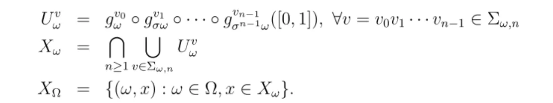
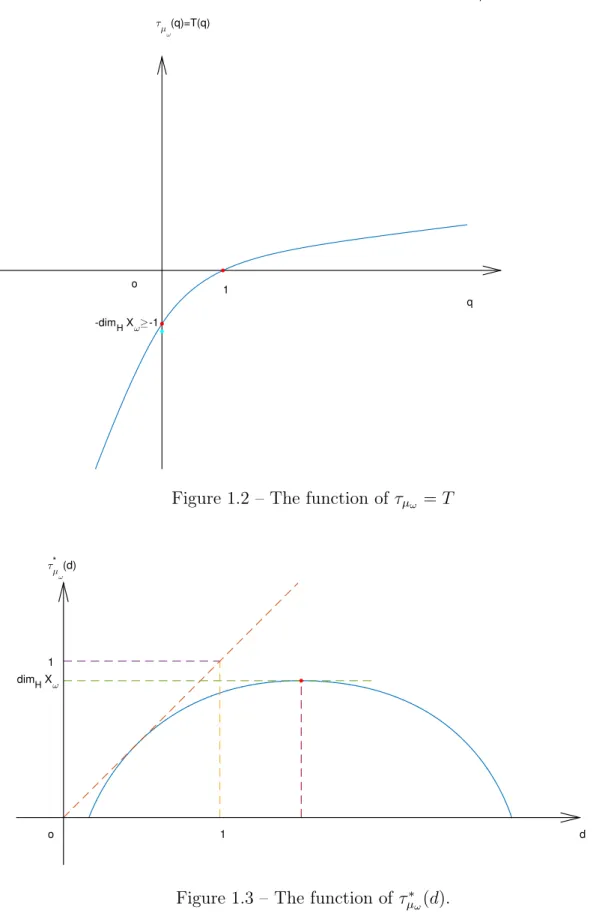
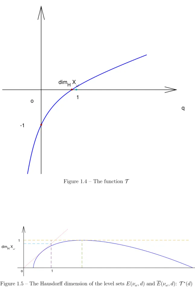
Here are some pictures describing the Legendre pairs (τµω, τµ∗ω) and (τνω, τν∗ω).
-dim H Xω≥-1 1 o q τ µ ω (q)=T(q)
Figure 1.2 – The function of τµω = T
dim H Xω 1 1 o d τ µ ω * (d)
Figure 1.3 – The function of τ∗ µω(d).
20 Multifractal analysis of the inverse of random weak Gibbs measures -1 1 dimH Xω o q
Figure 1.4 – The function T
1
1 dim
H Xω
o d
CHAPTER 1. INTRODUCTION 21
-1
dim
H
X
ω
1
o
q
Figure 1.6 – The Lq-spectrum for the inverse measure — τ νω 1 1 dim H Xω o d τ ν ω * (d)
22 Concrete examples of random attractors
1.6 Concrete examples of random attractors
The random attractors considered in this paper extend for instance the examples that are obtained if one considers the fibers of McMullen-Bedford self-affine carpets, and more generally the Gatzouras-Lalley self-affine carpets [82]. In particular, such fibers naturally illustrate the idea that at a given step of the construction two consecutive intervals Us
ω and Uωs+1 may touch each other. In [51], Luzia considers a
class of expanding maps of the 2-torus of the form f (x, y) = (a(x, y), b(y)) that are C2-perturbations of Gatzouras-Lalley carpets, whose fibers naturally illustrate our
purpose with nonlinear maps, but not C1. Also these examples are associated with
random fullshift.
Let us give more explicit examples. Here we use the notations of Section 1.2. A first example is the following. Let (Ω,F, P, σ) is the following:
Ω = Γ :=‹Z+׋Z+× · · · ,
F is the σ-algebra generated by the cylinders [n1n2· · · nk] for any k ∈ N and any
ni ∈ ˜Z+ for any i∈ N with 1 ≤ i ≤ k,
P([n1n2· · · nk]) = 1 n1(n1+ 1) · 1 n2(n2+ 1) · · · · · 1 nk(nk+ 1) ,
the map σ is the shift map. Such a system is ergodic. It satisfies the conditions we need.
Let n = n1n2· · · nk· · · ∈ Γ, define l(n) = n1 and A(n) = An1×n2, where An1×n2 is n1× n2-matrix with all entries equaling to 1 if n2 6= n2− 1 or n1 = 2, otherwise it
is a matrix satisfying that the entries of the first n1− 1 rows are 1 and the entries
of the n1-th row are 0 except that a(n1, n1 − 1) = 1. It is clear that such a system
can give us a random subshift system.
In fact it is easy to check that M and l are measurable. For any k∈ N, {n ∈ Ω : M(n) = k} = [(k + 1)k(k − 1) · · · 2],
and it is measurable. So that M is measurable. For l, for any k ∈ N, {n ∈ Ω : l(n) = k} = [k],
and it is also measurable.
Then l and M are unbounded butR log l dP < +∞, and we get a random subshift, which is not a fullshift . Now, we set Ti
n(x) = n1x mod 1 for x∈ [i−1n1 ,ni1] and for
i = 1, 2,· · · , n1.
For any point ω = n, If nk = 3, then at the k-th step the whole length of the
CHAPTER 1. INTRODUCTION 23
Poincaré’s recurrence theorem [83, theorem 1.4] or ergodic theorem [83, theorem 1.14], for P-almost every ω ∈ Ω, 3 will appear infinity many times, so at last the whole length (Lebesgue measure) will be 0 for the fiber at ω.
In fact, in the previous model the measure P is a special example of a Gibbs measure on the (Ω, σ) (see [78, 80]). So we can enrich the previous construction by considering any such measure P for whichR log l dP < +∞. For the mappings maps Ts
ω, here is a way to provide a non trivial example, which seems to be not covered
by the existing literature.
Start with a family{ϕs,ω}s∈N of random C1 differeomorphisms of [0, 1] such that
at least one ϕ′s,ω is nowhere Cǫ with positive probability. Assume that there exists
a random variable a0 taking values in (0, 1] and such that
inf
1≤s≤l(ω), x∈[0,1]|ϕ ′
s,ω(x)| ≥ a0(ω).
Let Ts
ω = ϕs,ω◦fωs, where fωs is the linear map from Uωsonto [0, 1]. Then, the constant
cψ of Assumption 1 satisfies cψ ≥ Z Ω " log(a0(ω))− sup 1≤s≤l(ω) log(|Uωs|) # dP(ω).
Thus, we require that
Z Ω " log(a0(ω))− sup 1≤s≤l(ω) log(|Us ω|) # dP(ω) > 0.
This allows some Ts
ω be not uniformly expanding, but ensures expansiveness
in the mean. It is easily seen that the Lebesgue measure of Xω is almost surely
bounded by Qni=0−1ÄP1≤s≤l(ω)|Us
σiω|/a0(σiω)
ä
for all n ≥ 1. Thus, if we strengthen our requirement by assuming that
Z Ω log(a0(ω))− log Ñ X 1≤s≤l(ω) |Us ω| é dP(ω) > 0,
then the Lebesgue measure of Xω is 0 almost surely.
Now let us provide a completely explicit illustration of the last idea (we will work with a random fullshift for simplicity of the exposition).
We take (Ω,F, P, σ) as the fullshift ({0, 1, 2}N,F, P, σ). For any n-th cylinder
[ω0ω1· · · ωn−1]⊂ Ω we set P([ω0ω1· · · ωn−1]) = 31n. It is the unique ergodic measure of maximal entropy for the shift map.
Let l be a random variable depending on ω0 only, which is given by
l(ω) = 4 ω0 = 0 1 ω0 = 1 3 ω0 = 2
24 Concrete examples of random attractors
The entries of the random transition matrix are always 1 (we consider the random fullshift). We assume that the map T (ω, x) just depends on ω0 and x.
If ω0 = 0, let ϕs,ω(x) = x for s = 1, 2, 3, 4 and Uω1 = [0, 1/4], Uω2 = [1/4, 1/2],
U3
ω = [1/2, 3/4] and Uω4 = [3/4, 1]. In this case, we know that a0(ω) = 1. By the
way the intervals Us
ω, 1 ≤ s ≤ 4 cover the interval [0, 1].
If ω0 = 1, let h(x) = 6 +P+j=1∞j−2sin(2jπx). Define
ϕ1,ω(x) = Rx 0 h(t)dt R1 0 h(t)dt , and U1
ω = [0, 1]. In this case we can choose a0(ω) = 1/2. It is easy to check that
T1
ω is not expanding on some interval; furthermore it is just of class C1 since h is
nowhere ǫ-Hölder for any ǫ∈ (0, 1).
If ω0 = 2, let ϕs,ω(x) = x for s = 1, 3 and ϕ2,ω(x) = 7x8 + x
2
8 , and U 1
ω = [0, 1/9],
U2
ω = [1/9, 2/9], Uω3 = [2/3, 7/9]. It is easy to check that the left derivative of Tω1 and
the right derivative of T2
ω is not coincide with each other, so it can not be express
as a conformal map here. In this case we can choose a0(ω) = 7/8.
Also, Z Ω log(a0(ω))− log Ñ X 1≤s≤l(ω) |Uωs| é dP(ω) = log 21− log 16 3 > 0,
Chapter 2
Basic properties of random weak
Gibbs measures
We will use the notations of the previous chapter. Fix a potential Φ∈ L1
ΣΩ(Ω, C(Σ)) (here P (Φ) may not be 0). Since varnΦ(ω)→ 0 as n→ 0 and (varnΦ)n≥1 is bounded in L1norm, using Maker’s ergodic theorem [54],
we can get
VnΦ(ω) := n−1X i=0
varn−iΦ(σiω) = o(n), P-almost surely. (2.1) Due to (1.3) and the ergodic theorem, setting SnkΦ(ω)k∞ = Pn−1i=0 kΦ(σiω)k∞, for
any positive sequence (an)n≥0 such that an = o(n) we have
SnkΦ(ω)k∞−Sn−ankΦ(ω)k∞
= nCΦ−(n−an)CΦ+o(n) = o(n), P-almost surely.
(2.2)
Definition 2.1 A family u = {un,ω : Σω,n → Σω} of measurable maps satisfying
(un,ω(v))|n = v for all v ∈ Σω,n and (n, ω) ∈ N × Ω is called an extension. We say
that it is measurable, if the map (ω, x) 7→ un,ω(x) is measurable for all n∈ N.
Let u ={un,ω} be an extension and Φ ∈ L1ΣΩ(Ω, C(Σ)). Then for (n, ω)∈ N × Ω Zu,n(Φ, ω) := X v∈Σω,n expÄSnΦ(ω, un,ω(v)) ä = X v∈Σω,n exp nX−1 i=0 Φ(Fi(ω, un,ω(v))) !
is called n-th partition function of Φ in ω with respect to u. Let
πn,u(Φ, ω) =
1
nlog Zu,n(Φ, ω). 25
26
Due to the assumption log(l)∈ L1(Ω, P), using the same method as in [35, 49], it is
easy to prove the following lemma.
Lemma 2.2 Let u be any extension and Φ∈ L1
ΣΩ(Ω, C(Σ)).
Then limn→∞πn,u(Φ, ω) = P (Φ) for P-almost every ω ∈ Ω. This limit is
inde-pendent of u.
Now let
λ(ω, n) = λ(ω)· λ(σω) · · · λ(σn−1ω),
where λ(ω) is defined as in proposition 1.1. The following lemma is direct when the potential Φ possesses bounded distorsions so that the Ruelle-Perron-Frobenious theorem holds for the operatorLω
Φ. For general potentials in L1ΣΩ(Ω, C(Σ)) we need a proof.
Lemma 2.3 One has lim
n→∞
log λ(ω, n)
n = P (Φ) for P-almost every ω∈ Ω.
Remark 2.4 In the following proof, as well as in the rest of this text, we will use the letter M to denote the levels of the function M(·). Keeping this in mind should prevent from some confusion.
Proof First, for M > 0, let FM = {ω ∈ Ω : M(ω) ≤ M}. Fix M large enough
so that P(FM) > 0. For each ω ∈ Ω, let bk(ω) be the k-th return time of ω to
the set AM. From ergodic theorem we get limk→∞ bkk = 1
P(FM) for P-almost every ω ∈ Ω. Then limk→∞ bk+1bk−bk = 0 for P-almost every ω ∈ Ω, which implies that M (σnω) = o(n).
Second, for any v∈ Σσnω we have
Zu,n−M(σnω))(Φ, ω) exp(−o(n)) ≤ Lω,n
Φ 1(v)≤ Zu,n(Φ, ω) exp(o(n)).
The right inequality uses the fact that we work with a subshift as well as (2.1). We just prove the left inequality: for n large enough so that M (σnω) ≤ n,
Lω,nΦ 1(v) = X w∈Σω,n,wv∈Σω exp(SnΦ(ω, wv)) ≥ X w′∈Σ ω,n−M (σnω) expÄSn−M(σnω)(ω, uω,n−M(σnω)(w′))− o(n) ä
= Zu,n−M(σnω))(Φ, ω) exp(−o(n)).
The inequality follows by using (1.2), then by preserving for each w′ ∈ Σ
ω,n−M(σnω) only one path of length M (σnω) from w′ to v, and by using (2.1), M (σnω) = o(n)
and (2.2).
Now, since λ(ω, n) =R Lω,nΦ 1(v)dµeσnω(v), we can easily get the result from lemma 2.2 and the fact that M (σnω) = o(n).
CHAPTER 2. BASIC PROPERTIES OF RANDOM WEAK GIBBS MEASURES 27
Proposition 2.5 Let u ={un,ω} be an extension and Φ, Ψ ∈ L1ΣΩ(Ω, C(Σ)). There exists Ω′ ⊂ Ω such that:
1. P(Ω′) = 1.
2. Setting Φq,t = qΦ− tΨ for (q, t) ∈ R2, for any ω ∈ Ω′, πn,u(Φq,t, ω) converges
uniformly to P (Φq,t) over the compact subsets of R2 as n → ∞.
Proof We first check that that πn,u(Φq,t, ω) is a convex function of (q, t):
For any (q1, t1), (q2, t2)∈ R2 and α∈ [0, 1]
πn,u(Φαq1+(1−α)q2,αt1+(1−α)t2, ω) = 1 nlog X v∈Σω,n exp(Sn(Φαq1+(1−α)q2,αt1+(1−α)t2)(ω, un,ω(v)) = 1 nlog X v∈Σω,n exp(Sn(αΦq1,t1 + (1− α)Φq2,t2)(ω, un,ω(v))) = 1 nlog X v∈Σω,n exp(Sn(αΦq1,t1)(ω, un,ω(v))· exp(Sn((1− α)Φq2,t2)(ω, un,ω(v))) ≤ α nlog X v∈Σω,n exp(Sn(Φq1,t1)(ω, un,ω(v))) + 1− α n log X v∈Σω,n exp(Sn(Φq2,t2)(ω, un,ω(v))) = απn,u(Φq1,t1, ω) + (1− α)πn,u(Φq2,t2, ω).
Fix a dense countable subset D of R2. For any (q, t) ∈ D, from theorem 2.2
we can find Ωq,t ⊂ Ω such that P(Ωq,t) = 1 and for any ω ∈ Ωq,t one has
limn→∞πn,u(Φq,t, ω) = P (Φq,t).
Let Ω′ = ∩
(q,t)∈DΩq,t. One has P(Ω′) = 1 and for any ω ∈ ΩC,
limn→∞πn,u(Φq,t, ω) = Pσ(Φq,t) for all (q, t) ∈ D. The uniform convergence over
the compact subsets of R2 is now a standard result in convex analysis (theorem 10.8
of [75]).
For each ω∈ Ω, let
D(ω) =: 1
λ(ω, M (ω))exp(−SM (ω)kΦ(ω)k∞).
Then D(ω) > 0 for P-almost every ω ∈ Ω. From M(σnω) = o(n), (2.2) and
lemma 2.3 we can get that log D(σnω) = o(n) P-almost surely.
Recall that by proposition 1.1, for P-a.e ω ∈ Ω, the measures µeω satisfy
(Lω
28
Proposition 2.6 For P-a.e ω ∈ Ω, for any n ∈ N, for all v = v0v1. . . vn−1 ∈ Σω,n,
one has D(σnω) λ(ω, n) exp ( infv∈[v]ω SnΦ(ω, v))≤µeω([v]ω)≤ 1 λ(ω, n)exp ( supv∈[v]ω SnΦ(ω, v)), so that exp(−ǫnn)≤ e µω([v]ω)
exp(SnΦ(ω, v)− log(λ(ω, n))) ≤ exp(ǫn
n) for any v ∈ [v]ω, where ǫn does not depend on v and tends to 0 as n → ∞.
Proof Let us deal first with the case n = 1.
Fix 1≤ i ≤ l(ω). For any 1 ≤ j ≤ l(σM (ω)ω), there exists w ∈ Σ
σω,M (ω)−1 such
that iwj ∈ Σω,1+M (ω). Due to proposition 1.1, we have
e µω([iwj]ω) = 1 λ(ω, M (ω)) Z Lω,M (ω)Φ 1[iwj]ωdµeσM(ω)ω, where Lω,nΦ =Lσn−1ω Φ ◦ · · · ◦ LσωΦ ◦ LωΦ. This implies e µω([iwj])≥
infw∈[iwj]ωexp(SM (ω)Φ(ω, w))
λ(ω, M (ω)) µeσM(ω)ω([j]σM(ω)ω).
Then µeω([i]) ≥ D(ω) follows after summing over 1 ≤ j ≤ l(σM (ω)ω). The upper
bound µeω([i])≤ 1 is obvious.
The general case is achieved similarly: If v ∈ Σω,n, for each 1 ≤ j ≤
l(σn+M (σnω)
−1ω), there exists w ∈ Σ
σnω,M (σnω)−1 such that vwj ∈ Σω,n+M (σnω). One has e µω([vwj]ω) = 1 λ(ω, n)λ(σnω, M (σnω)) Z Lω,n+M (σΦ nω)1[vwj]ωdµeσn+M (σnω)ω, from which we get
e µω([vwj]ω)≥ 1 λ(ω, n) · D(σ nω) exp ( inf v∈[v]ω SnΦ(ω, v))µeσn+M (σnω)ω([j]σn+M (σnω)ω). Then, taking the sum over 1≤ j ≤ l(σn+M (σnω)−1
ω) we get e µω([v]ω)≥ D(σnω) λ(ω, n) exp ( infv∈[v]ω SnΦ(ω, v)).
The inequality µeω([v]ω)≤ λ(ω,n)1 exp (supv∈[v]ωSnΦ(ω, v)) is direct from the equality
e µω([v]ω) = 1 λ(ω, n) Z Lω,nΦ 1[v]ωdµeσnω. Finally we conclude with (2.1) and log D(σnω) = o(n).
CHAPTER 2. BASIC PROPERTIES OF RANDOM WEAK GIBBS MEASURES 29 For any γ ∈ L1 XΩ(Ω,C([0, 1])) and any z‹ ∈ U v ω, let Snγ(ω, z) = nX−1 i=0 γ(σiω, vi, Tσvi−1i−1ω· · · Tωv0z).
Proposition 2.7 For P-almost every ω ∈ Ω, there are positive sequences (ǫ(ψ, n))n≥0 and (ǫ(φ, n))n≥0, that we also denote as (ǫ(Ψ, n))n≥0 and (ǫ(Φ, n))n≥0,
converging to 0 as n → +∞, such that for all n ∈ N, for all v = v0v1. . . vn ∈ Σω,n,
we have :
1. For all z ∈ ˚Uv ω,
exp(Snψ(ω, z)− nǫ(ψ, n)) ≤ |Uωv| ≤ exp(Snψ(ω, z) + nǫ(ψ, n)),
hence for all v ∈ [v]ω,
exp(SnΨ(ω, v)− nǫ(Ψ, n)) ≤ |Uωv| ≤ exp(SnΨ(ω, v) + nǫ(Ψ, n)).
Consequently, for all v ∈ Xv ω:
|Xv
ω| ≤ |Uωv| ≤ exp(SnΨ(ω, v) + nǫ(Ψ, n)).
2. For all v ∈ [v]ω,
exp(SnΦ(ω, v)− nǫ(Φ, n)) ≤µeω([v]ω)≤ exp(SnΦ(ω, v) + nǫ(Φ, n)),
hence for all z ∈ Uv ω,
exp(Snφ(ω, z)− nǫ(φ, n)) ≤ µω(Xωv) = µω(Uωv),
as well as µω(Uωv)≤ exp(Snφ(ω, z) + nǫ(φ, n)) if µeω is atomless.
Proof 1. For all n∈ N, for all v = v0v1· · · vn−1 ∈ Σω,n, define Tωv as
Tvn−1
σn−1ω◦ · · · ◦ Tσωv1 ◦ Tωv0. For any x, y∈ Uv
ω, from the Lagrange’s finite-increment theorem we have that
|Tv
ωx− Tωvy| = |(Tωv)′(z)||x − y|,
for some z between x and y. Since Tv
ω(Uωv) =: T vn−1 σn−1ω◦ · · · ◦ Tωv0(Uωv) = [0, 1], |Uωv| = 1 |(Tv ω)′(y)| = exp(Snψ(ω, z)),
30
for some z in the interior of Uv
ω. Then by definition (1.8) of cψ, due to the ergodicity
of the system (Ω,F, P, σ), we have sup
v∈Σω,n |Uv
ω| ≤ exp(kSnΨ(ω)k∞)≤ exp(−ncΨ/2) (2.3)
for n larger than some N (ω).
Let αn(ω) = var(ψ, ω, supv∈Σω,n|U
v ω|). Then, by definition of ψ, αn(ω) → 0 as n → ∞. Consequently, V (ψ, ω, n) := X 0≤i≤n αi(σn−iω) = o(n)
by Maker’s ergodic theorem, and the same holds for VnΨ(ω) which by definition
equals V (ψ, ω, n) (see (1.7) and (2.1)).
Since|Snψ(ω, z)− Snψ(ω, y)| ≤ V (ψ, ω, n) for any y, z ∈ Uωv, we get
exp(Snψ(ω, z)− o(n)) ≤ |Uωv| ≤ exp(Snψ(ω, z) + o(n))
for all z ∈ ˚Uv
ω. The inequality associated with SnΨ follows immediately.
2. Noting that we reduced the situation to P (Φ) = 0, the first part of this item comes from theorem 2.6, lemma 2.3, proposition 2.6, the fact that D(σnω) =
o(n), and the control (2.1) of the distorsion VnΦ coming from the assumption φ ∈
L1XΩ(Ω,C([0, 1])).‹
Chapter 3
Basic properties of random Gibbs
measures
Random Gibbs measures are associated with random Hölder continuous potentials. We say that a function Φ is a random Hölder potential if Φ is measurable from ΣΩ
to R, Z
sup
v∈Σω
|Φ(ω, v)|dP < ∞, and there exists κ∈ (0, 1] such that
varnΦ(ω)≤ KΦ(ω)e−κn, (3.1)
where the random variable KΦ = KΦ(ω) > 0 is such that
R
log KΦ(ω)dP(ω) <∞.
A random Hölder continuous potential is obviously in L1
ΣΩ(Ω, C(Σ)).
Theorem 3.1 ([48, 49]) Assume that F is a countably generated σ-algebra, F is a topological mixing subshift of finite type and Φ a random Hölder potential.
For P-almost every ω ∈ Ω, there exists some random variables C = CΦ(ω) > 0,
λ = λΦ(ω) > 0, a function h = h(ω) = h(ω, v) > 0 and a measure µe ∈ M1 P(ΣΩ)
with disintegrationsµeω satisfying
Z
| log CΦ| dP < +∞, Z | log λΦ| dP < +∞ and log h is a Hölder potential,
and such that
Lω
Φh(ω) = λ(ω)h(σω), (LωΦ)∗µeσω= λ(ω)µeω,
Z
h(ω) dµeω = 1. (3.2)
Let mω = mΦω be given by dmω = h(ω)dµeω and set dm(ω, v) = dµeω(v)dP(ω).
Then m ∈ I1
P(ΣΩ), for P-almost every ω ∈ Ω, for all v = v0v1. . . vn−1 ∈ Σω,n, and
32
for all v ∈ [v]ω
1 CΦ ≤
mω([v]ω)
exp(Pni=0−1Φ(Fi(ω, v))− log λΦ(σn−1ω)· · · λΦ(ω)) ≤ C
Φ. (3.3)
The family of measures (mω)ω∈Ω is called a random (or relative) Gibbs measure
(or state) for the potential Φ. Moreover, m is the unique maximizing F -invariant probability measure in the variational principle, i.e. such that
P (Φ) = hF(m|P) +
Z
Φ dm, and one has P (Φ) =
Z
log λ(ω) dP. (3.4)
Each time we need to refer to the function Φ, we denote the measures m and mω
as mΦ and mΦ
ω, and denote λ as λΦ.
We can also define the random Gibbs measure on the random attractor Xω by setting
µω = mω◦ πω−1.
In this thesis if the potential Φ (which is related to φ) is a random Hölder potential, then when we say the relative measures mΦ
ω and µφω, they are referred to
be random Gibbs measures.
Given a random Hölder potential Φ, from (3.2) we can define the normalized potential Φ′(ω, v) = Φ(ω, v) + log h(ω, v)− log h(F (ω, v)) − log λ(ω), which satisfies
Lω
Φ′1 = 1 for P-almost every ω ∈ Ω. This implies that Φ′ ≤ 0 for P-almost every ω ∈ Ω. Also, we have the following fact:
Proposition 3.2 Suppose that Φ is a random Hölder potential. If P (Φ) = 0, there exist some ̟ > 0 such that for P-almost every ω ∈ Ω, there exists N(ω) such that for any n ≥ N(ω) and any v ∈ Σω,n, one has
sup
v∈[v]ω
SnΦ(ω, v)≤ −n̟.
As a consequence, µω is atomeless.
If we need to refer explicitly to Φ, we will use the notations NΦ(ω) and ̟Φ instead
of N (ω) and ̟.
The main idea of the proof is from [31].
Proof Since P (Φ) = 0, we have sup{R Φ dρ : ρ∈ IP(ΣΩ)} ≤ 0.
We claim that sup{R Φ dρ : ρ ∈ IP(ΣΩ)} < 0. Let M large enough such that
P({ω : M(ω) < M, l(ω) ≥ 2}) > 0. For any ω ∈ Ω such that M(ω) < M and l(ω) ≥ 2 we haveLω,MΦ′ 1 = 1, hence SMΦ′(ω, v) < 0 for any v ∈ Σω and
R
SMΦ′(ω, v)dρω < 0
for any probability measure ρω on Σω. Since, moreover, we have SMΦ′ ≤ 0, we
CHAPTER 3. BASIC PROPERTIES OF RANDOM GIBBS MEASURES 33
Let −2̟ := sup{R Φ dρ : ρ ∈ M1
P(ΣΩ, F )}. If the proposition does not hold,
there exists a subsequence (nk)k≥1 such that
#{v : |v| = nk, supv∈[v]ωSnkΦ(ω, v) nk >−̟} ≥ 1. For any q ∈ R+, P (qΦ) = lim k→∞ logPv∈Σω,nkexpÄqSnkΦ(ω, unk,ω(v)) ä nk ≥ limk →∞ −q̟nk nk =−q̟. However, P (qΦ) = sup ρ∈M1 P(ΣΩ,F ) ß hρ(F ) + Z qΦ dρ ™ ≤ sup ρ∈M1 P(ΣΩ,F ) ßZ qΦ dρ ™ + sup ρ∈M1 P(ΣΩ,F ) {hρ(F )} ≤ −2q̟ + sup ρ∈M1 P(ΣΩ,F ) {hρ(F )} Since supρ∈M1 P(ΣΩ,F ){hρ(F )} = R
log l dP <∞, letting q tend to ∞ we get a contra-diction.