HAL Id: hal-02081549
https://hal.archives-ouvertes.fr/hal-02081549
Submitted on 27 Mar 2019
HAL is a multi-disciplinary open access
archive for the deposit and dissemination of
sci-entific research documents, whether they are
pub-lished or not. The documents may come from
teaching and research institutions in France or
abroad, or from public or private research centers.
L’archive ouverte pluridisciplinaire HAL, est
destinée au dépôt et à la diffusion de documents
scientifiques de niveau recherche, publiés ou non,
émanant des établissements d’enseignement et de
recherche français ou étrangers, des laboratoires
publics ou privés.
First-Half Index Base For Querying Data Cube
Viet Phan-Luong
To cite this version:
Viet Phan-Luong. First-Half Index Base For Querying Data Cube. Intelligent Systems Conference
2018, Sep 2018, London, United Kingdom. �10.1007/978-3-030-01054-6_78�. �hal-02081549�
First-Half Index Base For Querying Data Cube
Viet Phan-LuongAix-Marseille Univ, Universit´e de Toulon, CNRS, LIS, Marseille, France Equipe BDA
Email: [email protected]
Abstract—Given a relational fact table R, we call a base of data cubes on R a structure that allows to query the data cubes with any aggregate function. This work presents a compact base of data cubes, called the first-half index base, with its implementation, and the method for querying the data cubes using this base. Through experiments on real datasets, we show how the first-half index base resolves efficiently the main data cube issues, i.e., the storage space and the query response time.
Keywords-data warehouse; data cube; data mining; I. INTRODUCTION
The concept of data cube offers important interests to business intelligence as it provides aggregate views of data over multiple combinations of dimensions. Those aggregate views can help managers to make appropriate decision in their business. In fact, a data cube built on a relational fact table with
n dimensions and a measure M for an aggregate function g
can be seen as the set of the Structured Query Language (SQL) group-by queries over the power set of the n dimensions,
where g is applied to each group of measures M . The result
of such a SQL group-by query is an aggregate view, called a cuboid.
Though the concept is simple, there are many important issues in computation time and storage space, because of the exponential number of the cuboids and because of the big size of large datasets. To make data cube query available in Online Analytical Processing (OLAP), most solutions to reduce the time computation are to precompute the data cube and store it on disk. However, the storage space can be tremendous.
To tackle these issues, there exist many different approaches. In [9], an I/O-efficient technique based upon a multiresolution wavelet decomposition is used to build an approximate and space-efficient representation of data cubes. Naturally, the response to an OLAP query is also approximate. The iceberg data cube approach [8][10][20] [22] does not compute all aggregates, but only those above certain thresholds. This approach does not allow all data cube queries because data cubes are partially computed.
The other approaches search to represent the entire data cube with efficient methods for computation and storage [1][2][7][18]. The computing time and storage space are optimized based on equivalence relations defined on aggregate functions [11] [19] or on the concept of closed itemsets in frequent itemset mining [17] or by reducing redundancies between tuples in cuboids, using tuple references [2] [11][15] [16][19][21][23]. In these approaches, the computation is usually organized on the complete lattice of sub-schemes of
the fact table dimension scheme. The computation can traverse the complete lattice in a top-down or bottom-up manner. To create cuboids, the sort operation is used to reorganize tuples: tuples are grouped and the aggregate functions are applied to the measures. To optimize the storage space, only aggregated tuples with aggregated measures are directly stored on disk. Non-aggregated tuples are not stored but represented by references to the stored tuples where the non aggregated tuples are originated or to tuples in the fact table. The work [23] implemented many of these approaches and reported the experimental results on real and synthetic datasets. It shown that The Totally-Redundant-Segment BottomUpCube approach (TRS-BUC) nearly dominated its competitors in all aspects of the data cube problem: fast computation of a fully materialized cube in compressed form, incrementally updateable, and quick query response time.
The work [12][13] presents a simple and reduced represen-tation that allows to compute efficiently the entire data cubes for any aggregate functions. The main idea in this work is that among the cuboids of a data cube, there are ones that can be easily and rapidly get from the others, with no important computing time. These others are computed and stored on disk using an integrated binary search prefix tree structure for compact representation and efficient search. In contrast to the approaches that compute all tuples of the data cube with optimization in computing time and storage space, the work [13] computes and represents only the cuboids of a half of data cube, called the last-half data cube. It follows a special top-down approach that does not traverse the complete lattice of the dimension sub-schemes: from each cuboid in the last-half data cube, over a dimension schemeX, we can compute, with
no important time cost, a non-stored cuboid over a dimension sub-scheme Y ⊂ X, using an operation called aggregate
projection. The set of those non-stored cuboids is called the first-half data cube.
Moreover, the above proposed representation is not only for a specific aggregate function, nor for a specific measure, but it allows for computing all cuboids with any measure and any aggregate function. In fact, each cuboid in the representation is an index: a set of rowids that reference to tuples in the fact table.
In the present work, we extend [13] in a somehow contrast direction, by studying a more compact and efficient represen-tation that allows to speed up the compurepresen-tation of data cube queries. The contribution consists of:
com-putation, and
– The methods for computing the data cube queries based on this compact representation.
The efficiency of the representation in run time and storage space is shown through experiments on four real datasets.
The paper is organized as follows. Section 2 recalls the main concepts in [13], in particular, the concept of the first-half and the last-half data cubes. Section 3 presents the concepts of the new representation for querying data cubes. Section 4 presents the methods for computing the group-by query with aggregate functions, based on this representation. Section 5 reports the experimental results and ends with discussions. Finally, conclusion and further work are in Section 6.
II. PRELIMINARY
This section recalls the main concepts presented in [13]. A data cube over a dimension scheme R is the set of cuboids
built over all subsets of R, that is the power set of R. As in
most of existing work, dimensions (attributes) are encoded in integer, let us consider R = {1, 2, ..., n}, n ≥ 1. The power
set of R can be recursively defined as follows.
1) The power set of R0= ∅ (the empty set) is P0= {∅}. 2) For n ≥ 1, the power set of Rn = {1, 2, ..., n} can be
recursively defined as follows:
Pn= Pn
−1∪ {X ∪ {n} | X ∈ Pn−1} (1)
Pn−1 is called the first-half power set of Rn and the second operand ofPn, i.e.,{X ∪ {n} | X ∈ Pn−1}, the
last-half power set ofRn.
Example 1: For n = 3, R3= {1, 2, 3}, we have:
P0= {∅}, P1= {∅, {1}}, P2= {∅, {1}, {2}, {1, 2}},
P3= {∅, {1}, {2}, {1, 2}, {3}, {1, 3}, {2, 3}, {1, 2, 3}}. The first-half power set of S3 is P2 = {∅, {1}, {2},
{1, 2}} and the last-half power set of S3 is
{{3}, {1, 3}, {2, 3}, {1, 2, 3}}, got by adding 3 to each
element of P2.
The set of all cuboids over the schemes in the first-half power set ofR is called the first-half data cube and the set of
all cuboids over the schemes in the last-half power set of R
is called the last-half data cube.
In [12][13], the last-half data cube is precomputed and stored on disks and data cube queries are computed based on the last-half data cube. However, it proposed a more general framework: instead of computing for a data cube for a particular aggregate function, it computes and stores the tuples indexes over the schemes in the last-half power set ofR, and
data cube queries for any aggregate function are computed based on these indexes.
From now on we consider a relational fact table T with a
dimension scheme R = {1, 2, ..., n} and a set of measures M = {n + 1, n + 2, ..., n + k}.
III. THE FIRST-HALF INDEX BASE FOR DATA CUBES In the present work, we follow the view of data cube as the composition of two parts: the last-half and the first-half.
To improve the computing time and the storage space of the data cube representation, we shall follow an approach that is somehow inverse to the approach proposed in [12][13]. Indeed, in the new approach, the first-half data cube is computed and stored on disk. It forms a base to compute all data cube queries. For this, we define a data structure and some algorithms.
A. Data indexes on an attribute
Data on a dimension (an attribute) of the fact table T is
indexed using the search binary tree structure. This structure has following fields:
– data : to contain an attributed value,
– ltid : to contain the list of rowids associated with the
attributed value,
– lsib and rsib: the left and the right sub-trees.
The structure is organized for searching on the data field. We call a tree with this structure an attribute index tree.
To insert attributed values into an attribute index tree, we use the algorithm InsData2AttIndex.
Algorithm InsData2AttIndex:
Input: An attributed value val, the rowid of a tuple that
containsval, and an attribute index tree P .
Output: The attribute index treeP updated.
Method:
if (P == NULL) {
Create P with P.data = val;
Create P.ltid with the 1st element rowid; P.lsib = NULL and P.rsib = NULL;
}
else if P.data > val {
insert val and rowid into P.lsib; }
else if P.data < val {
insert val and rowid into P.rsib); }
else append rowid to P.ltid); }
Such attribute index trees (and further index trees) are stored on disk. As each index is a partition of the set of all rowids of T, it is important to note that, to optimize the storage space of these indexes, we save only the partitions of rowids and omit the attributed values.
B. Tuples indexes on a dimension scheme
Given a sub-scheme {A1, ..., Ak} (for 1 ≤ i ≤ n, 1 ≤
Ai ≤ n) of the dimension scheme R of the fact table T , we assume that the index over {A1, ..., Ak−1} is already created for all tuples ofT . As the base, the indexes over the schemes {1}, ..., {n} are created using the InsData2AttIndex algorithm.
LetP be an element of the index over {A1, ..., Ak−1}. That is,P is the list of all rowids of the tuples that have the same
value on{A1, ..., Ak−1}; these tuples may be different on Ak. To create the index of tuples on {A1, ..., Ak}, we use the algorithmT upleIndex.
Algorithm TupleIndex:
Input: the fact tableT and a dimension scheme {A1, ..., Ak}.
Method:
1. Get the tuple index over {A1, ..., Ak−1}
2. For each P in the index on {A1, ..., Ak −1}
do
2.1 Initialize a tree T rP to empty;
2.2 For each rowid in P do
2.2.1 Let val be the attributed value on Ak of the tuple at rowid in T;
2.2.2 Insert val and rowid to T rP using
2.2.2 the InsData2AttIndex algorithm; 2.2.3 done;
2.3 Write the tree T rP to disk;
3. done;
To access to the tuple at the row identified byrowid in the
fact table T , we organize the data as follows. The fact table T is loaded into a list of blocks in the main memory. Each
block is an array of fixed size k. To determine the number of
the block that contains the tuple atrowid and the rang of the
tuple in the block:
blocknumber = rowid / k rang = rowid % k,
where/ and % denote respectively the quotient and the rest
of the division on integers.
C. Creating the first-half index base
The indexes of tuples over the schemes in the first-half power set of the dimension scheme of the fact table T are
generated by the algorithm GenIndexF H.
Algorithm GenFHIndex:
Input:T and its dimension scheme {1, ..., n}.
Output: The tuple indexes for the first-half data cube over
{1, ..., n} and their dimension sub-schemes.
Method:
Let RS be a list of dimension sub-schemes, initially empty;
1. Use InsData2AttIndex to generate n indexes over schemes {1}, ..., {n} and append
successively these schemes to RS.
2. Set a pointer psch to the 1st scheme in RS
and let P be the pointed scheme (at this point, P is {1}); 3. len= 1;
4. while len < n and psch6= N U LL do
4.1. Let lastAtt be the last attribute of P
4.2. For each attribute i from 1 to n− 1
such that i > lastAtt do
4.2.2 Append i to P to create a new scheme
nsc and append nsc to RS;
4.2.4 Use T upleIndex to generate the tuple index over nsc;
4.2.5 Save the tuple index to disk; 4.2.6 done;
4.3 Set psch to the next element in RS and
len= length(nsc); 4.4 done;
5. Return RS.
Each scheme in RS is associated with the information that
allows to identify the corresponding tuple index stored on disk.
D. First-half index base representation for data cube
Based on the tuple indexes over the schemes in the first-half power set of the fact table dimension scheme, we propose a representation, called the first-half index base for query-ing data cube on T . The first-half index base is the triple (T, RS, F HIndex), where
– RS is the return of GenF HIndex(T ) and
– F HIndex is the set of tuple indexes generated by GenF HIndex(T ).
The above elements are stored on disks. For efficient com-puting, the list of dimension schemesRS and the fact table T
are retrieved in the main memory. The fact table T is stored
in a list of blocks of fixed size as explained previously. IV. DATACUBEQUERY BASED ON THE FIRST-HALF INDEX
REPRESENTATION
This section explains how we can compute the queries with the aggregate functions MAX, COUNT, SUM, AVERAGE, and VARIANCE, based on the first-half index base.
A. Query on the first-half cube
To compute a cuboid on an aggregate function g, over a
scheme F in the first-half data cube, we access to the tuple
index overF , and for each partition P of rowids of this index:
– Letrowid1 be the first rowid in P and let t be the tuple
atrowid1.
– Lett(F ) be the restriction of t on F ,
– Let M be the set of the measures that we can get from T for all rowids in P ,
– Apply the aggregate function g to M , let g(M ) be the
result,
– Savet(F ) and g(M ) to disk.
For computing the function VARIANCE, for each partition
P , we use a temporary list to store the measures in the tuples
at allrowids ∈ P .
B. Query on the last-half cube
The algorithm QueryLH computes a cuboid in the last-half data cube, over a scheme L, based on the tuple index
over F = L − {n} where n is the last attribute of the
dimension scheme. This tuple index is in the first-half index base(T, RS, F HIndex).
Algorithm QueryLH:
Input: A dimension sub-scheme L = {A1, ..., Ak, n}, an aggregate functiong, and (T, RS, F HIndex).
Output: the cuboid onT and g, over L.
Method:
1. Get the tuple index over F = L − {n} from
F HIndex;
2. For each partition P in the index over F do 2.1 Initialize a tree T rP to empty;
2.2 For each rowid in P do
2.2.1 Let val be the value on attribute n
of the tuple at rowid in T; 2.2.2 Insert val and rowid to T rP
using InsData2AttIndex; 2.2.3 done;
tuple t at the rowid at the root of T rP,
and,
and g(T rP) the result of the application
of g to the set of measures in all tuples at the rowids in T rP;
2.4 Save t(F ) and g(T rP) to disk;
2.5 done;
V. EXPERIMENTAL RESULTS AND DISCUSSIONS The first-half index base for data cube query is implemented in C and experimented on a laptop with 8 GB memory, Intel Core i5-3320 CPU @ 2.60 GHz x 4, running Ubuntu 12.04 LTS. The experimentation is done on four real datasets CovType [3], SEP85L [4], STCO-MR2010 AL MO [5] and
OnlineRetail [6]
CovType is a dataset of forest cover-types. It has 581,012 tuples on ten dimensions with cardinality as follows: Horizontal-Distance-To-Fire-Points (5,827), Horizontal-Distance-To-Roadways (5,785), Elevation (1,978), Vertical-Distance-To-Hydrology (700), Horizontal-Distance-To-Hydrology (551), Aspect (361), Hillshade-3pm (255), Hillshade-9am (207), Hillshade-Noon (185), and Slope (67).
SEP85L is a weather dataset. It has 1,015,367 tuples on nine dimensions with cardinality as follows: Station-Id (7,037), Longitude (352), Solar-Altitude (179), Latitude (152), Present-Weather (101), Day (30), Present-Weather-Change-Code (10), Hour (8), and Brightness (2).
STCO-MR2010 AL MO is a census dataset on population of Alabama through Missouri in 2010, with 640,586 tuples over ten integer and categorical attributes. After transforming categorical attributes (STATENAME and CTYNAME), the dataset is reorganized in decreasing order of cardinality of its attributes as follows: RESPOP (9,953), CTYNAME (1,049), COUNTY (189), IMPRACE (31), STATE (26), STATENAME (26), AGEGRP (7), SEX (2), ORIGIN (2), SUMLEV (1).
OnlineRetail is a data set that contains the transactions occurring between 01/12/2010 and 09/12/2011 for a UK-based and registered non-store online retail. This dataset has incom-plete data, integer and categorical attributes. After verifying, transforming categorical attributes into integer attributes, for the experiments, we retain 393,127 complete data tuples and the following ten dimensions ordered in their cardinality as follows: CustomerID (4,331), StockCode (3,610), UnitPrice (368), Quantity (298), Minute (60), Country (37), Day (31), Hour (15), Month(12), and Year (2).
A. On building the first-half index base of data cube
Table I reports the run time and the memory use for computing the first-half index bases and their store space. In this table,
– the term “Run time” means the time (in seconds) from the start of the program until the first-half index base is completely built, including the time to read/write input/output files.
– the term “Memory use” means the maximal space of the main memory allocated to the program, from the start until the first-half index base is completely built.
– the term “Storage space” means the volume in mega bytes to store the first-half index base on disks.
TABLE I
RESULTS ON COMPUTING FIRST-HALF BASE
Datasets Run time Memory use Storage space
CoveType 138s 90 Mo 2 Go
SEP85L 127s 170 Mo 1.8 Go
STCO-... 141s 125 Mo 2.2 Go
OnlineRetail 96s 80 Mo 1.4 Go
B. On query with aggregate functions
The group-by SQL queries are computed based on the first-half index base. The following aggregate functions MAX, COUNT, SUM, AVG, and VARIANCE are experimented. The queries are in the following simple form:
Select ListOfDimensions, f(m) From Fact_Table
Group by ListOfDimensions;
For each dataset and each half of the corresponding data cube, the query is computed for all cuboids in the half. For instance, for CovType, we run the above query for 512 cuboids of the last-half and 512 cuboids of the first-half.
Tables II and III show the total time in seconds for comput-ing the aggregate query for the five aggregate functions, for all cuboids in the first-half data cubes and in the last-half data cubes, respectively. The total times include all computing and i/o time, in particular, the time to write the results to disk. For instance, for the aggregate function SUM, the total time for computing 512 cuboids in the first-half data cube of dataset CovType is 237 seconds (Table II). The last column (MEAN) represents the average of the total time on the five aggregate functions.
TABLE II
TOTAL TIME FOR COMPUTING AGGREGATE QUERY ON FIRST-HALF CUBES
DATASETS MAX COUNT SUM AVG VAR MEAN
CoveType 235s 215s 237s 302s 288s 255.4 s
SEP85L 140s 118s 141s 169s 170s 147.6 s
STCO-... 144s 126s 144s 170s 176s 152 s
OnlineRetail 117s 106s 117s 145s 144s 125.8 s
TABLE III
TOTAL TIME FOR COMPUTING AGGREGATE QUERY ON LAST-HALF CUBES
DATASETS MAX COUNT SUM AVG VAR MEAN
CoveType 309s 279s 364s 383s 373s 341.6 s
SEP85L 193s 169s 191s 224s 237s 202.8 s
STCO-... 184s 168s 184s 212s 228 195.2 s
OnlineRetail 150s 146s 158s 180s 183s 163.4 s
Table IV shows the average time in seconds to compute the response to an aggregate query. The data in this table is computed based on the data in Tables II and III. For each half of a data cube, the average time is calculated by dividing the total time by the number of cuboids in the half.
For instance, for the first-half data cube of CoveType, the average query response time for SUM is 237s/512 = 0.46
second, and for the five aggregate functions the average query response time is 255.4s/512 = 0.50 second. For
the entire data cube, the average query response time for SUM is (237s + 364s)/1024 = 0.59 second, and for the
five aggregate functions the average query response time is (255.4s + 341.6s)/1024 = 0.58 second.
TABLE IV
AVG RESPONSE TIMES OF AGGREGATE QUERY
ON FIRST-HALF CUBES
DATASETS MAX COUNT SUM AVG VAR MEAN
CoveType 0.46 0.42 0.46 0.59 0.56 0.50
SEP85L 0.55 0.46 0.55 0.66 0.66 0.58
STCO-... 0.28 0.25 0.28 0.33 0.34 0.30
OnlineRetail 0.23 0.21 0.23 0.28 0.28 0.25
ON LAST-HALF CUBES
DATASETS MAX COUNT SUM AVG VAR MEAN
CoveType 0.60 0.54 0.71 0.75 0.73 0.63
SEP85L 0.75 0.66 0.75 0.88 0.93 0.79
STCO-... 0.36 0.33 0.36 0.41 0.45 0.38
OnlineRetail 0.29 0.29 0.31 0.35 0.36 0.32
ON ENTIRE CUBES
DATASETS MAX COUNT SUM AVG VAR MEAN
CoveType 0.53 0.48 0.59 0.67 0.65 0.58
SEP85L 0.65 0.56 0.65 0.77 0.80 0.68
STCO-... 0.32 0.29 0.32 0.37 0.39 0.34
OnlineRetail 0.26 0.25 0.27 0.32 0.32 0.28
C. Discussions
To get some ideas on the efficiency of the first-half index base approach, we show in this section the experimental results on CoveType and SEP85L of the present approach and those of the last-half data cube representation [13][14] and of the very competitive method TRS-BUC [23]. In the discussion, we shall show (i) the implementation and the reported measures in the experimentation of the approaches, and (ii) their common and different points.
The last-half data cube representation approach is imple-mented in the same conditions as the first-half index base approach. After [23], TRS-BUC is implemented on a PC Pen-tium 4, 2.80 Ghz, running Windows XP. The results reported for TRS-BUC are the storage space and the construction time of the representation and the average query response time (avg QRT) based on the representation. However, [23] did not precise whether the construction time and the average query response time include the time to write the result to disk. In contrast, in [13][14] and the present work, all time reported includes the i/o time, in particular, the time to write the data result (cuboids) to disk. Moreover, in Table V, the avg QRT of [13][14] and the present work is the average on the five aggregate functions MAX, COUNT, SUM, AVG, and VARIANCE.
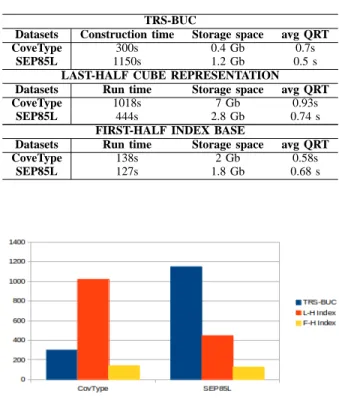
Table V synthesizes the main experimental results of the first-half index base with views on the results of the last-half data cube representation and those of the TRS-BUC method. The data in this table is graphically represented in Figures 1,
2, and 3. In each graph, the three columns, from left to right, represent respectively the results of the TRS-BUC method, the last-half data cube representation, and the first-half index base representation.
TABLE V
MAIN RESULTS WITH VIEWS ON PREVIOUS WORK
TRS-BUC
Datasets Construction time Storage space avg QRT
CoveType 300s 0.4 Gb 0.7s
SEP85L 1150s 1.2 Gb 0.5 s
LAST-HALF CUBE REPRESENTATION
Datasets Run time Storage space avg QRT
CoveType 1018s 7 Gb 0.93s
SEP85L 444s 2.8 Gb 0.74 s
FIRST-HALF INDEX BASE
Datasets Run time Storage space avg QRT
CoveType 138s 2 Gb 0.58s
SEP85L 127s 1.8 Gb 0.68 s
Fig. 1. Construction/Run times of three methods in seconds
Fig. 2. Storage space of the representations in giga bytes The common point between the first-half index base ap-proach and the last-half data cube representation apap-proach is that the both approaches use a half of the data cube index to represent the entire data cube. The different points:
a) One uses the first-half and the other uses the last-half. In general the volume of the last-half data cube is bigger than the volume of first-half data cube.
b) The first-half index base approach follows the bottom-up computation, whereas the last-half data cube representation approach follows the top-down computation.
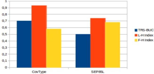
Fig. 3. Average query response times of three methods in seconds
c) In the first-half index base approach, as the representation of data cube, only the partitions of rowids are stored on disk, but no data tuples (tuples over dimension sub-schemes). In the last-half data cube representation approach, both data tuples and the partitions of rowids are stored on disk.
By above points b) and c), the reduction of the storage space and the run time to build the first-half index base with respect to the storage space and the run time to build the last-half data cube representation is considerable: on storage space, about 71% for CoveType and 35% for SEP85L, and on run
time, about 86% for CoveType and about 71% for SEP85L.
Though these important reductions, the average query response time is clearly improved by the first-half index base.
The difference between the above approaches and TRS-BUC consists in:
– TRS-BUC computes the entire data cube and optimizes the storage space of tuples: if an aggregate group has only one tuple, then the tuple itself is not stored, but only the rowid of its original tuple in the fact table: the rowid is called a reference. The approaches [13][14] optimize the storage by representing the data cube by a half cube of indexes.
– TRS-BUC computes the representation of the data cube built on a specific aggregate function applied to only one measure: for each aggregated tuple, only one aggregated value of the measure is stored. Whereas the representations by a half of data cube compute the index bases for computing data cube with any aggregated function: for each aggregated tuple, a partition of rowids is stored. This explains why the storage space of the representation by a half of data cube is much more bigger than that of TRS-BUC.
VI. CONCLUSION AND FURTHER WORK On the above discussions, we can see that
– The first-half index base representation is really more efficient than the last-half data cube representation, in terms of storage space, construction time, and average query response time, and
– We can not really compare experimental results of the last-half data cube representation or the first-half index base with those of TRS-BUC, because they are not defined and computed in the same conditions.
However, on the results in Table V, we can see that the first-half index base can be a competitive approach to TRS-BUC,
as it builds the bases in very reduced time, with respect to the construction time of TRS-BUC, and offers the avg QRT that is almost comparable to that of TRS-BUC. Moreover, based on the first-half index base, the data cube query can be computed with any measure and any aggregate functions, without recomputing the representation.
For further work, we plan to test the first-half index base on much larger datasets and to study its incremental construction.
REFERENCES
[1] S. Agarwal et al., “On the computation of multidimensional aggregates”, Proc. of VLDB’96, pp. 506-521.
[2] V. Harinarayan, A. Rajaraman, and J. Ullman, “Implementing data cubes efficiently”, Proc. of SIGMOD’96, pp. 205-216.
[3] J. A. Blackard, “The forest covertype dataset”, ftp://ftp. ics.uci. edu/pub/machine-learning-databases/covtype.
[4] C. Hahn, S. Warren, and J. London, “Edited synoptic cloud re-ports from ships and land stations over the globe”, http://cdiac. esd.ornl.gov/cdiac/ndps/ndp026b.html.
[5] 2010 Census Modified Race Data Summary File for Counties Alabama through Missouri http://www.census.gov/popest/research/modified/ STCO-MR2010 AL MO.csv.
[6] Online Retail Data Set, UCI Machine Learning Repository, https://archive.ics.uci.edu/ml/datasets/Online+Retail,
[7] K. A. Ross and D. Srivastava, “Fast computation of sparse data cubes”, Proc. of VLDB’97, pp. 116-125.
[8] Beyer, K.S., Ramakrishnan, R.: Bottom-up computation of sparse and iceberg cubes, Proc. of ACM Special Interest Group on Management of Data (SIGMOD’99), 359-370.
[9] J. S. Vitter, M. Wang, and B. R. Iyer, “Data cube approximation and histograms via wavelets”, Proc. of Int. Conf. on Information and Knowledge Management (CIKM’98), pp. 96-104.
[10] J. Han, J. Pei, G. Dong, and K. Wang, “Efficient Computation of Iceberg Cubes with Complex Measures”, Proc. of ACM SIGMOD’01, pp. 441-448.
[11] L. Lakshmanan, J. Pei, and J. Han, “Quotient cube: How to summarize the semantics of a data cube,” Proc. of VLDB’02, pp. 778-789. [12] V. Phan-Luong, “A Simple and Efficient Method for Computing Data
Cubes”, Proc. of The 4th Int. Conf. on Communications, Computation, Networks and Technologies INNOV 2015, pp. 50-55.
[13] V. Phan-Luong, “A Simple Data Cube Representation for Efficient Computing and Updating”, Int. Journal on Advances in Intelligent Systems, vol 9 no 3 & 4, 2016, pp. 255-264. http://www.iariajournals.org/intelligent systems.
[14] V. Phan-Luong, “Searching Data Cube for Submerging and Emerging Cuboids”, Proc. of The 2017 IEEE Int. Conf. on Advanced Information Networking and Applications Science AINA 2017, IEEE, pp. 586-593. [15] Y. Sismanis, A. Deligiannakis, N. Roussopoulos, and Y. Kotidis, “Dwarf:
shrinking the petacube”, Proc. of ACM SIGMOD’02, pp. 464-475. [16] W. Wang, H. Lu, J. Feng, and J. X. Yu, “Condensed cube: an efficient
approach to reducing data cube size”, Proc. of Int. Conf. on Data Engineering 2002, pp. 155-165.
[17] A. Casali, R. Cicchetti, and L. Lakhal, “Extracting semantics from data cubes using cube transversals and closures”, Proc. of Int. Conf. on Knowledge Discovery and Data Mining (KDD’03), pp. 69-78. [18] A. Casali, S. Nedjar, R. Cicchetti, L. Lakhal, and N. Novelli,
“Loss-less Reduction of Datacubes using Partitions”, In Int. Journal of Data Warehousing and Mining (IJDWM), 2009, Vol 5, Issue 1, pp. 18-35. [19] L. Lakshmanan, J. Pei, and Y. Zhao, “QC-Trees: An Efficient Summary
Structure for Semantic OLAP”, Proc. of ACM SIGMOD’03, pp. 64-75. [20] D. Xin, J. Han, X. Li, and B. W. Wah, “Star-cubing: computing iceberg
cubes by top-down and bottom-up integration”, Proc. of VLDB’03, pp. 476-487.
[21] Y. Feng, D. Agrawal, A. E. Abbadi, and A. Metwally, “Range cube: efficient cube computation by exploiting data correlation”, Proc. of Int. Conf. on Data Engineering 2004, pp. 658-670.
[22] Z. Shao, J. Han, and D. Xin, “Mm-cubing: computing iceberg cubes by factorizing the lattice space”, Proc. of Int. Conf. on Scientific and Statistical Database Management (SSDBM 2004), pp. 213-222. [23] K. Morfonios and Y. Ioannidis, “Supporting the Data Cube Lifecycle: