CHAOS IN A THREE-DIMENSIONAL VOLTERRA-GAUSE MODEL OF PREDATOR-PREY TYPE

HAL Id: hal-01026173

https://hal-univ-tln.archives-ouvertes.fr/hal-01026173

HAL is a multi-disciplinary open access archive for the deposit and dissemination of sci-entific research documents, whether they are pub-lished or not. The documents may come from

L’archive ouverte pluridisciplinaire HAL, est destinée au dépôt et à la diffusion de documents scientifiques de niveau recherche, publiés ou non, émanant des établissements d’enseignement et de

CHAOS IN A THREE-DIMENSIONAL

VOLTERRA-GAUSE MODEL OF PREDATOR-PREY

TYPE

Jean-Marc Ginoux, Bruno Rossetto, Jean-Louis Jamet

To cite this version:

Jean-Marc Ginoux, Bruno Rossetto, Jean-Louis Jamet. CHAOS IN A THREE-DIMENSIONAL VOLTERRA-GAUSE MODEL OF PREDATOR-PREY TYPE. International journal of bifurcation and chaos in applied sciences and engineering , World Scientific Publishing, 2005, 15 (5), pp.1689. �10.1142/S0218127405012934�. �hal-01026173�

CHAOS IN A THREE-DIMENSIONAL

VOLTERRA-GAUSE MODEL OF

PREDATOR-PREY TYPE

JEAN-MARC GINOUX, BRUNO ROSSETTO AND JEAN-LOUIS JAMET

PROTEE Laboratory, University of South Toulon Var, B.P. 20132,

83957, LA GARDE Cedex, France

CHAOS IN A THREE-DIMENSIONAL

VOLTERRA-GAUSE MODEL OF

PREDATOR-PREY TYPE

JEAN-MARC GINOUX, BRUNO ROSSETTO AND JEAN-LOUIS JAMET

PROTEE Laboratory, University of South Toulon Var, B.P. 20132,

83957, LA GARDE Cedex, France

E-mail:

ginoux@univ-tln.fr

,

rossetto@univ-tln.fr

,

jamet@univ-tln.fr

Abstract

The aim of this paper is to present results concerning a three-dimensional model including a prey, a predator and top-predator, which we have named the Volterra-Gause because it combines the original model of V. Volterra incorporating a logisitic limitation of the P.F. Verhulst type on growth of the prey and a limitation of the G.F. Gause type on the intensity of predation of the predator on the prey and of the top-predator on the top-predator. This study highlights that this model has several Hopf bifurcations and a period doubling cascade generating a snail shell-shaped chaotic attractor.

With the aim of facilitating the choice of the simplest and most consistent model a comparison is established between this model and the so-called Rosenzweig - MacArthur and Hastings-Powell models. Many resemblances and differences are highlighted and could be used by the modellers.

The exact values of the parameters of the Hopf bifurcation are provided for each model as well as the values of the parameters making it possible to carry out the transition from a typical phase portrait characterising one model to another (Rosenzweig-MacArthur to Hastings-Powell and vice versa).

The equations of the Volterra-Gause model cannot be derived from those of the other models, but this study shows similarities between the three models.

In cases in which the top-predator has no effect on the predator and consequently on the prey, the models can be reduced to two dimensions.

Under certain conditions, these models present slow-fast dynamics and their attractors are lying on a slow manifold surface, the equation of which is given.

1. Introduction

The paper is organized as follows. In the following section we will study a three-dimensional Volterra-Gause* model in the most general case. The stability of the fixed points according to the works of Freedman and Waltman [1977] and the occurrence of Hopf bifurcation in this model are examined. This analysis shows that such a bifurcation exists in the xy plane and is possible apart from the xy plane.

Then, the study of the Volterra-Gause model for particular values of parameters (k = p = 1/2), checking for the existence of bifurcations in the xy plane and apart from the xy plane and determining the values of the bifurcation parameters.

Dynamic analysis of this particular case demonstrate the existence of a chaotic attractor in the shape of a snail shell.

The bifurcation diagrams indicates the existence of a period doubling cascade leading to chaos.

The section ends with another particularly dynamical aspect which is, that under certain conditions, this model presents slow-fast dynamics.

So, according to the works of Ramdani et al., [2000], we give the slow manifold equation of the surface on which trajectories of the attractor are lying on.

The aim of the last section is to compare the most used predator – prey models.

We begin by summarising the general properties of the Rosenzweig-MacArthur [1963] and Hastings-Powell [1991] models, including the stability of fixed points, the value of the Hopf bifurcation parameter and the equation of the slow manifold surface.

In the Hastings-Powell [1991] model, we show, against expectations, that some of the trajectories of the so-called “teacup” also lie on a surface.

Similarities in behaviour between these three models are highlighted:

the nature and number of fixed points, type of bifurcation, shape of the attractor.

Variation of a parameter to obtain a Hopf bifurcation also makes it possible to emphasize a transition from one model to another.

Indeed, the modification of certain parameter values for a given model can be used to determine the behavior phase portrait of another model.

This comparison exhibits that the phase portrait of the Volterra-Gause model can be transformed into that of the Hastings-Powell [1991] model and vice versa.

Similarly, the phase portrait of the Rosenzweig-MacArthur [1963] model can be transformed into a “teacup” and vice versa.

The phase portrait of the Volterra-Gause model is similar to that of Rosenzweig-MacArthur [1963] in a number of respects.

These results are potentially of great value to modellers as they provide a panoply of models that are "equivalent" in terms of phase portrait but differents in terms of dynamic.

* Strictly, in the general case this model should be called the Volterra-Rosenzweig model because the functional

response corresponds to that used by M.L. Rosenzweig in his famous article: Paradox of enrichment [Rosenzweig, 1971]. However, to avoid confusion with the Rosenzweig-MacArthur [1963] model we prefer to use the name of G.F. Gause, who was the first to use this kind of functional response but in a particular case [Gause, 1935] corresponding to the object of our study.

2. General Volterra-Gause Model

2.1. Model equations

We consider the Volterra-Gause model for three species interacting in a predator-prey mode.

d x d t = aJ1− λa xNx−b x k y=x gHxL−b y pHxL d y d t =d x k y−c y−e ypz =y@−c+d pHxLD−e z qHyL H1L d z d t =Hf y p₋ gLz=z@−g+f qHyLD

This model consists of a Verhulst [1838] logistic functional response for the prey (x), and a Gause [1935] functional response for the predator (y), and for the top-predator (z).

Parameter a is the maximum per-capita growth rate for the prey in the absence of predator and a / l is the carrying capacity.

The per-capita predation for the predator rate is of the Gause [1935] type.

pHxL= xk

Parameter b is the maximum per-capita predation rate.

Parameter c is the per-capita natural death rate for the predator.

Parameter d is the maximum per-capita growth rate of the predator in the absence of the top-predator.

Parameters e is similar to b, except that, in each case, the predator y is the prey for the top-predator z.

2.2. Dynamic aspects

The non-algebraic structure of the polynomials forming the right hand side of the equations (1) make it impossible to determine the fixed points by the classical nullclines method. However, this model possesses two obvious fixed points: O (0, 0, 0), K (a / l, 0, 0).

This makes it possible to look for fixed points within the xy plane, by fixing z = 0.

Nullcline analysis of the system (1) identifies the point I, with the following co-ordinates:

Ii k jjJc dN 1 k_, d b c J c dN 1 kA_a− λ Jc dN 1 kE_{, 0}y { zz

2.2.2. Conditions of existence of the fixed points in the xy plane (CEFP 2D)

Fixed points are only of biological importance if they are positive or null. This generates the following condition: a− λ Jc dN 1 k >_{0 d}J a λN k −c >0 H2L

2.2.3. Functional Jacobian matrix

1Hx, y, zL= i k jjjj jjj a−b k x−1+k_y−_{2 x}λ −_{b x}k ₀ d k x−1+ky −c+d xk−e p y−1+pz −e yp 0 f p y−1+p_z −_g+_{f y}p y { zzzz zzz=i_kjjjjj m11 m12 m13 m21 m22 m23 m31 m32 m33 y { zzzz z H3L

2.2.4. Nature and stability of the fixed points in the xy plane

The point O (0, 0, 0), with eigenvalues {a, -c, -g}, is unstable (a > 0), attractive according to y'y and z'z and repulsive according to x'x.

The point K (a / l, 0, 0), with eigenvalues {-a, -g, -c + d (a / l)k}, is unstable (-c + d (a / l)k > 0, according to (2)), attractive according to x'x and z'z and repulsive according to:

y= − a−c+dIa λM k bIa λMk x= −κx

because according to (2): -c + d(a / l)k > 0 and thus k > 0

The method described by Freedman and Waltman [1977] can be used to study the stability of the point Ii k jjJc dN 1 k_, d b c J c dN 1 kA_a− λ Jc dN 1 kE_{, 0}y { zz

The characteristic polynomial of the functional Jacobian matrix can be factorised in the following form:

Hm33− σL Iσ2−m11σ −m12m21M=0 ; m13 = m31=m32= m22=0

and provides three eigenvalues: s1, s2 and s3

σ1=m33= −g+f yp H4L

The sign of the first of these eigenvalues cannot be determined under any condition and it is therefore impossible to draw conclusions concerning the stability.

For the other two eigenvalues, resolution of the second-order polynomial provides a pair of eigenvalues s2 and s3. σ2,3= m11±è!!!!∆ 2 = m11±"#########################m112 +4m12m21 2 H5L

If we assume that D < 0, then the two eigenvalues are complex conjugated.

For Hopf bifurcation to occur, the real part of these eigenvalues must be positive and cancelled for a certain value of a parameter.

Let us choose l this parameter and calculate the real part of these eigenvalues.

2Re@σ2D=m11=a−b k x−1+ky−2 xλ =AH1−kL bc d y− λx 2_EJ1 xN As a - lx2 = bxk y and xk = c / d

Re[s2] > 0 if and only if (1- k)y bc/d - lx2¥0, providing a condition for y

y≥ d

bc λ1−k x

2

by replacing x and y by the co-ordinates of I

λ ≤aJ1−k 2−kN J c dN −1 k H₆L

One can demonstrate that whatever the parameters of the model the discriminant D is always negative. Thus the point I is always a stable or unstable focus.

2.2.5. Conditions for the existence of a Hopf bifurcation in the xy plane

Provided that l remains below this value and the first eigenvalue (4) is negative, so that the associated eigendirection is attractive and the flow is directed towards the basin of attraction of the point I, a limit cycle exists in the xy plane and a Hopf bifurcation may occur in that plane. The point

Ii k jjJc dN 1 k_, d b c J c dN 1 kA_a− λ Jc dN 1 kE_{, 0}y { zz is then unstable, and acts as an attractive focus in the xy plane.

2.2.6. Fixed points in the first octant

We will now investigate the existence of fixed points in the first octant with biological significance, i.e., for z > 0.

The non-algebraic form of the right hand side of the first equation of (1) precludes solution by means of analytical calculation.

Nevertheless, expressing this polynomial as a function of x makes it possible to specify the number of fixed points and the interval in which they belong. There are only two possible solutions to this non-algebraic polynomial.

We will call these two solutions x1,2 = a. They lie in the following interval:

x1<x∗< a λ J 1−k 2−kN<x2< a λ H7L

According to the third equation of (1), the second co-ordinate y can be expressed as follows: Hf yp−gLz=0 y=Jg fN 1 p If we set β =y=Jg fN 1 p

from the second equation of (1), the third co-ordinate z can be expressed in terms of x:

−c y+d xky−e ypz=0 z= fβ e g Id x

k₋

cM

2.2.7. Conditions for the existence of fixed points in the first octant (CEFP 3D)

From this third co-ordinate, another condition for the biological relevance of the fixed point can be determined.

d xk−c>0 x>Jc dN

1

k H₈L

The fixed point J can therefore be defined in terms of all of its co-ordinates, and the conditions justifying its biological existence.

Ji k jjα,β, fβ e gIdα k₋ cMy { zz with x>Jc dN 1 k H₉L

A bifurcation can only occur apart from the xy plane if there is no possible bifurcation in the xy plane. This can be translated into a condition deduced from the following inequality (7):

λ ≥aJ1−k 2−kN J c dN −1 k a λ J 1−k 2−kN≤J c dN 1 k H₁₀L

By combining inequalities (7) and (9), we obtain:

x1<x∗< a λ J 1−k 2−kN<J c dN 1 k <_x 2< a λ H11L

2.2.8. Nature and stability of the fixed points in the first octant

The method descibed by Freedman and Waltman [1977] can still be used to investigate the stability of the point

Ji k jjα,β, fβ e g Idα k₋ cMy { zz

According to this method, if m11 > 0, then the point J is unstable.

If m11 < 0 and m22 § 0, then the point J is stable.

Furthermore, if m11 < 0, then the point J is asymptotically stable.

The trace and the determinant of the functional Jacobian matrix evaluated at point J give:

σ1+ σ2+ σ3=Tr@1D=m11+m22

=aH1−kL− λxH2−kL+H1−pLI−c+d xkM

σ1 σ2 σ3=Det@1D=m11m23m32

=@aH1−kL− λxH2−kLDAe g p yp−1zE

=@aH1−kL− λxH2−kLDI−c+d xkMg p

2.2.9. Conditions for the existence of a Hopf bifurcation in the first octant

Based on the conditions for the biological existence of a fixed point J (CEFP 3D), we can conclude:

If x1 is the solution of the first nullcline, then the point J does not exist because, according to

condition (11), x1< (c/d)1/k and therefore z1<0. A Hopf bifurcation may then occur at point I

in the xy plane if the first eigenvalue (4) is negative. In this case, the associated eigendirection is attractive and the flow is directed towards the basin of attraction of the point I. This is consistent with condition (6), which implies that:

x1<J c dN 1 k < _x∗< a λ J 1−k 2−kN

If x2 is the solution of the first nullcline, then the point J exists because according to the condition (11), x1<x∗< a λ J 1−k 2−kN<J c dN 1 k < _x 2< a λ

In this case, points I and J co-exist and it is necessary to determine the stability of J, even if the first eigenvalue (4) is positive, resulting in the associated eigendirection being repulsive and the flow being directed towards the basin of attraction of the point J.

Nevertheless in this precise case: m11 = a (1 - k) - l x2 (2 - k) < 0.

This implies that the determinant is negative and the sign of the trace is unspecified because we deal with a difference.

If we assume that the characteristic polynomial of the functional Jacobian matrix has two complex conjugated eigenvalues, the trace and the determinant will be written:

σ1+2Re@σ2D=Tr@1D

σ1»σ2»2= Det@1D<0

We can deduce from these expressions that the first eigenvalue is negative. Thus the associated eigendirection is attractive and the flow is directed towards the basin of attraction of the point J. Moreover, the indeterminate nature of the sign of the trace is consistent with the possibility that the real part of the eigenvalues can change. Thus, in this case, the possibility of Hopf bifurcation apart from the xy plane may be considered.

2.3. Volterra-Gause model for k = p = 1/2

Expressing equations in a dimensionless form makes it possible to reduce the number of parameters of the model.

Let us assume: x→ a λ x y→ a b J a λN 1 2 _y z→ d e J a bN 1 2 Ja λN 3 4 _z t→ t dIa λM 1 2 and

δ1= c d 1 Ia λM 1 2 δ2= 1 f g Aa b I a λM 1 2E 1 2 ξ = d a J a λN 1 2 ∂= f d I a bM 1 2 Ia λM 1 4

This generates a dimensionless model with four parameters instead of eight. In fact, as we have decided to set k = p =1/2, the final model actually has six parameters rather than eight.

ξ dx dt =xH1−xL−x 1 2 _y dy dt = −δ1y+x 1 2 _y−_y 1 2 _z H₁₂L dz dt =∂ i k jjy 1 2 − δ₂y { zzz

2.3.2. Fixed points of dimension in the xy plane

The two previously identified fixed points are again found: O (0, 0, 0) and K (1, 0, 0).

In addition, the setting of the k and p parameters makes it possible to solve the first nullcline simply by changing variable.

However, the method developed above remains valid and exact knowledge of the solutions of this equation is not necessary for determination of the stability of the fixed points.

It is therefore possible to look for fixed points in the xy plane by setting z = 0 for k = p = 1/2. This gives the following co-ordinates of point I:

IIδ₁2,δ1I1−δ12M, 0M

2.3.3. Conditions for the existence of fixed points in the xy plane (CEFP 2D)

Fixed points are only of biological significance if they are positive or null. This generates the following condition:

2.3.4. Functional Jacobian matrix 1Hx, y, zL= i k jjjj jjjj jjjj jjjj 1 ξ J1−2 x− 12 y è!!!!_x N −1_ξ è!!!!x 0 1 2 y è!!!!_x è!!!!x − 1₂ è!!!!!z_y − δ1 −è!!!!y 0 1 2 ∂ z è!!!!!_y ∂Iè!!!!y − δ2M y { zzzz zzzz zzzz zzzz= i k jjjj j m11 m12 m13 m21 m22 m23 m31 m32 m33 y { zzzz z H14L

2.3.5. Nature and stability of the fixed points in the xy plane

The point O (0, 0, 0), with the eigenvalues {1/x, -d1, -∂d2}, is unstable (1/x > 0), and the

eigendirections associated with the eigenvalues -d1, -∂d2 are attractive according to y'y and

z'z and repulsive according to x'x for 1/x.

The point K (1, 0, 0), with the eigenvalues {-1/x, 1-d1, -∂d2}, is unstable (1-d1 > 0,

according to (10)), and the eigendirections associated with the eigenvalues -1/x, -∂d2 are

attractive according to x'x and z'z and repulsive according to the direction of the straight line defined by the following equation:

y= −@ξ H1− δ1L+1Dx

The method of Freedman and Waltman[1977] can again be used to assess the stability of the point

IIδ₁2,δ1I1−δ12M, 0M

The characteristic polynomial of the functional Jacobian matrix can be factorised in the following form:

Hm33− σL Iσ2−m11σ −m12m21M=0 ; m13 = m31=m32= m22=0

and provides three eigenvalues: s1, s2 and s3 σ1=m33=∂Aδ1 1 2 _{I1− δ} 1 2_M1_{2 − δ} 2E H15L

For the first eigenvalue, the conditions for the existence of a fixed point in the first octant (CEFP 3D) make it possible to define the sign of the eigenvalue, and therefore to draw conclusions concerning the stability. For the other two eigenvalues, resolution of the secon-order polynomial gives a pair of eigenvalues, s2 and s3.

σ2,3=

m11±è!!!!∆

2 =

m11±"#########################m112 +4m12m21

2 H16L

If we assume that D < 0, then the two eigenvalues are then complex conjugated.

For Hopf bifurcation to occur, the real part of these eigenvalues must be positive and cancelled for a certain value of a parameter.

Let us choose d1 this parameter and calculate the real part of these eigenvalues. 2Re@σ2D=m11= 1 ξ I1−3 δ12M≥0 δ1≤ 1 è!!!!₃ H17L

For this bifurcation occurs in the xy plane, the first eigenvalue (15) must be negative, so that the associated eigendirection is attractive and the flow is directed towards the basin of attraction of point I.

If this eigenvalue is considered as a function of d1, one can show that it will remain negative

provided that:

δ2≥&''''''''''''''

2

3è!!!!3 H 18L

This condition rules out the existence of a point J in the first octant. 2.3.6. Conditions for the existence of a Hopf bifurcation in the xy plane

If conditions (17) and (18) are met, a limit cycle exists in the xy plane and a Hopf bifurcation may occur in that plane. Point J of dimension three cannot exist and the point

IId₁2,d₁I1- d₁2M, 0M _{is unstable. It acts as an attracive focus in the xy plane.}

2.3.7. Fixed points in the first octant

We will now focus on the existence of fixed points of biological importance in the first octant, i.e., for z > 0. We can specify the number of solutions of the non-algebraic polynomial of the first equation (12) and the interval in which they lie as described above.

We will once again call the two possible solutions x1,2 = a these solutions. These solutions lie

in the following interval:

0<x1<x∗<

1

3 <x2<1

Mathematical study of the first nullcline as a function of x generates the following condition for the existence of the fixed points in the first octant (CEFP 3D):

δ2≤&''''''''''''''

2

3è!!!!3 H 19L

From the third equation of (12), the second co-ordinate y may be expressed as follows:

∂i k jjy 1 2 − δ₂y { zz=0 y= δ₂2

From the second equation of (12), the third co-ordinate z can be expressed in terms of x: −δ1y+x 1 2 _y−_y 1 2 _z=_{0 z}= δ₂i k jjx 1 2 − δ₁y { zz

2.3.8. Conditions for the existence of fixed points in the first octant (CEFP 3D)

From this third co-ordinate, we can deduce another condition for the biological existence of the fixed point:

x 1 2 − δ₁>_{0 x}> δ 1 2 _H 20L

The fixed point J can therefore be defined in terms of its co-ordinates in all three dimensions and the conditions justifying its biological existence.

Ji k jjα,δ₂2,δ2i k jjα12− δ₁y { zzy { zz with x> δ₁2 H21L

If a bifurcation is to occur apart from the xy plane, bifurcation must not be possible in the xy plane. This translates into a condition that can be deduced from inequality (17):

δ1> 1 è!!!! 3 or 1 è!!!!₃ > 1₃ By combining inequalities (20) and (21), we obtain:

x1<x∗<

1

3 < δ1<x2<1 H22L

2.3.9. Nature and stability of the fixed points in the first octant

The method of Freedman and Waltman [1977] can be used to study the stability of the point

Ji k jjα,δ₂2,δ2i k jjα12− δ₁y { zzy { zz

According to this method, if m11 > 0, then the point J is unstable.

Furthermore, if m11 < 0, then the point J is asymptotically stable.

The trace and the determinant of the functional Jacobian matrix evaluated at point J give:

σ1+ σ2+ σ3=Tr@1D=m11+m22= 1 2 ξ H1−3xL+ 1 2 i k jjx 1 2 − δ₁y { zz σ1 σ2 σ3=Det@1D=m11m23m32= ∂ 2ξ H1−3 xLz

2.3.10. Conditions for the existence of a Hopf bifurcation in the first octant

From the conditions for the biological existence of the fixed point J (CEFP 3D), we can conclude:

If x1 is the solution of the first nullcline, then point J does not exist because according to

condition (22), x1 < d1 and therefore z1 < 0.

A Hopf bifurcation may occur in the xy plane at point I if the first eigenvalue (15) is negative. In this case, the associated eigendirection is attractive and the flow is directed towards the basin of attraction of point I, consistent with condition (17), which implies that:

x1< δ1< x∗<

1 3

If x2 is the solution of the first nullcline, then the point J exists because according to condition

(22),

0< x1<x∗<

1

3 < δ1< x2<1

In this case, points I and J co-exist and it is necessary to determine the stability of J, even if the first eigenvalue (15) is positive, resulting in the associated eigendirection being repulsive and the flow being directed towards the basin of attraction of the point J.

Nevertheless in this precise case: 1-3x < 0.

This implies that the determinant is negative and the sign of the trace is unspecified as we are dealing with a difference.

If we assume that the characteristic polynomial of the functional Jacobian matrix has two conjugated complex eigenvalues, then the trace and the determinant can be expressed as follows:

σ1+2Re@σ2D=Tr@1D

σ1»σ2»2= Det@1D<0

We can deduce from this that the first eigenvalue is negative, so the associated eigendirection is attractive and the flow is directed towards the basin of attraction of the point J. Moreover, the indeterminate nature of the sign of the trace makes it possible for the real part of the eigenvalues to change. Hopf bifurcation apart from the xy plane may therefore be considered.

2.3.11. Bifurcation parameter value

Numerically, the value of the selected bifurcation parameter can be calculated with a high level of accuracy. The technique used involves calculating the fixed points according to the parameter and evaluating the eigenvalues of the functional Jacobian matrix at this point. These eigenvalues are thus themselves a function of the selected parameter. Their real parts can therefore be expressed as a function of this parameter, making it possible to determine the value for which two of these eigenvalues cancel out, corresponding to the value of the bifurcation parameter. Applied to system (12) by setting x = 0.866, ¶ = 1.428, d2 = 0.376, we

obtained for the parameter d1:

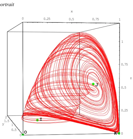
d1 = 0.747413 2.3.12. Phase portrait 0 0.25 0.5 0.75 1 x 0 0.5 1 1.5 2 y 0 0.25 0.5 0.75 1 z O I J K

Fig. 1. Phase portrait of system (12). The chaotic attractor takes the shape of a snail shell. Parameter values are: x = 0.866, ¶ = 1.428, d1 = 0.577, d2 = 0.376.

Despite its familiar appearance, this attractor behaves in a complex manner.

Following the repulsive eigendirection y = -[x (1 - d1) + 1] x of the point K, the flow reaches

the basin of attraction of the point I, which exhibits an attractive focus behaviour in the xy plane and turns around the point I.

However, as this point has a repulsive eigendirection, the flow leaves the xy plane and moves towards the basin of attraction of the point J which has an attractive eigendirection.

As the point J behaves as a repulsive focus, the flow turns around this point while moving away in the direction of the point K which has an attractive eigendirection according to z'z. The flow is therefore "reinjected" by this "saddle-point".

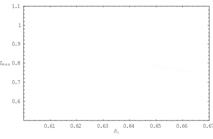
2.3.13. Bifurcation diagrams

As pointed out by Glass and Mackey [1988], the construction of a bifurcation diagram is a good means of locating the signature of chaos in a system.

We present below the bifurcation diagram of the dimensionless system (12) to highlight the period doubling induced by the parameter d1.

0.61 0.62 0.63 0.64 0.65 0.66 0.67 δ1 0.6 0.7 0.8 0.9 1 1.1 Zm a x

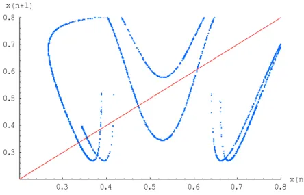
2.3.13. Poincaré section and Poincaré map

The Poincaré section corresponds here to a plane with z = 1/2, i.e., a plane dividing the snail shell into two parts. It therefore consists of a set of x and y values.

Taking x (n) as the value of x at the nth intersection of the trajectory with the Poincaré section, we can construct the Poincaré map: the function relating x (n + 1) to x (n)

In Fig. 3., we can see that the slope of the multimodal Poincaré map is steep, a feature typical of chaos. 0.3 0.4 0.5 0.6 0.7 0.8 xHnL 0.3 0.4 0.5 0.6 0.7 0.8 xHn+1L

2.4. Slow-fast dynamics

Given all the condtions for the existence of fixed points (CEFP 2D & 3D), it is reasonable to assume "trophic time diversification" occurs, implying that:

a > d > f

i.e., the maximum per-capita growth rate decreases from the bottom to the top of the food chain.

We can then consider the case in which:

a á d á f

or

0 < x Ü 1

and

0< ¶ Ü 1

Under these conditions, system (12) becomes a singularly perturbed system of three time scales.The rates of change for the prey, the predator and top-predator from fast to intermediate to slow, respectively [B.Deng,2001]. Based on the works of Ramdani et al., [2000], we consider system (12) to be a slow-fast autonomous dynamic system defined by a slow manifold equation on which the attractor lies. A state equation binding the three variables can then be established.

2.4.1. Slow manifold equation based on the orthogonality principle

Using the method developped by Ramdani et al., [2000], we can obtain the slow manifold equation defined by the layer of planes locally orthogonal to the fast eigenvector on the left.

λ1Hx, y, zLzλ₁H1,β Hx, y, zL,γ Hx, y, zLL

Let us call l1(x, y, z) the fast eigenvalue of 1 (x, y, z) and zl1(1, b(x, y, z), g(x, y, z)) the fast

eigenvectors on the left of 1(x, y, z). Transposing the characteristic equation,

t_{H1Hx, y, zLLz}

λ1Hx, y, zL= λ1Hx, y, zLzλ1Hx, y, zL

we can find b and g.

β = 1 1 2 x −1 2 _y i k jjλ1− 1 ξ ikjj1−2 x− 1 2 x −1 2 _yy { zzy { zz γ = β y 1 2 i jj 1 yzz

The slow manifold equation is thus given by:

x‰+ β Hx, y, zLy‰+ γ Hx, y, zLz‰=0 H23L

This leads to an implicit equation which can be simulated numerically. We have used Mathematica software in this study.

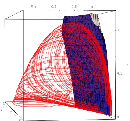
0.2 0.4 0.6 0.8 1 x 0 0.5 1 1.5 2 y 0 0.5 1 z

Fig. 4. Slow manifold surface based on the orthogonality principle and phase portrait of the Volterra-Gause system (12) with the same parameter values. In this figure, we can see the slow manifold on which the solutions of the system (12) are based.

2.4.2. Slow manifold equation based on the slow eigenvectors

The slow manifold equation could also have been obtained as descibed by Ramdani et al., [2000], by assuming that the three components of the system (12) are always parallel to a plane containing the two slow eigenvectors.

2.5. Conclusion

This work demonstrates the presence of chaos in a Volterra-Gause model of predator-prey type. Nevertheless, a more profound mathematical approach, such as investigation of the possible existence of Shilnikov orbits, should make it possible to confirm the presence of chaos in this system. Our work has also demonstrated that this model has five key characteristics:

- Presence of limit cycles - Existence of Hopf bifurcation - Chaos by period doubling cascade - Slow-fast dynamics

- Existence of a slow manifold on which the attractor lies.

The Volterra-Gause model is also similar to other models, such as those of Rosenzweig-Mac Arthur and Hastings and Powell. These similarites will be considered in the next section.

3. Similarity to the Rosenzweig-MacArthur and

Hastings-Powell Models

3.1. Rosenzweig-MacArthur model

We considered the Rosenzweig-MacArthur model [1963] for a three trophic level interaction involving a prey (x), a predator (y) and a top-predator (z).

d x d t =aJ1− λa xNx− b x y H1+x = x gHxL−b y pHxL d y d t =y i k jj d x H1+x − cy { zz− e y z H2+y = y@−c+d pHxLD−e z qHyL H24L d z d t =z i k jj f y H2+y − gy { zz=z@−g+f qHyLD

This model includes a Verhulst [1838] logistic prey (x), a Holling [1959] type 2 predator (y), and a Holling [1959] type 2 top-predator (z).

Parameter a is the maximum per-capita growth rate for the prey in the absence of predator and K = a / l is the carrying capacity.

The per-capita predation rate of the predator has the Holling [1959] type 2 form.

pHxL= b x H1+x

Parameter b is the maximum per-capita predation rate and H1 is the semi-saturation constant

at which the per-capita predation rate is half its maximum, b/ 2. Parameter c is the per-capita natural death rate for the predator.

Parameter d is the maximum per-capita growth rate of the predator in the absence of the top-predator.

Parameters e and H2 are similar to b and H1, except that the predator y is the prey for the

top-predator z. Parameters f and g are similar to c and d, except that the top-predator y is the prey for the top-predator z.

Note that the Rosenzweig-MacArthur model was developed from the seminal works of Lotka [1925] and Volterra [1926].

3.1.1. Dimensionless equations

With the following changes of variables and parameters,

t d t, x λ a x, y bλ a2 y, z b eλ d a2 z, ξ = d a,∂= f d,β1= λ H1 a ,β2= H2 Y0 , Y0= a2 bλ,δ1= c d,δ2= g f

3.1.2. Biological hypothesis

We have made several assumptions to provide biological reality to our study: - Positivity of the fixed points

- "Trophic time diversification hypothesis" such that the maximum per-capita growth rate decreases from the bottom to the top of the food chain as follows

a > d > f > 0

We also assumed major changes over time

a á d á f > 0 (25)

Detailed comments on changes in variables and parameters were made in the paper by Deng [2001]. For technical reasons, both y and z were rescaled by a factor of 0.25:

y ö y / 0.25 ; z ö z / 0.25

Equations (24) have been reformulated in the following dimensionless form:

ξ dx d t =x i k jj1−x− y β1+x y { zz d y d t =y i k jj x β1+x − δ 1− z β2+y y { zz H26L d z d t =∂z i k jj y β2+y − δ 2y { zz 3.1.3. Dynamic aspects

Under these conditions (25), the system (26) becomes a singularly perturbed system of three time scales, as previously pointed out by several authors [Kuznetsov, 1995, Muratori & Rinaldi, 1992, Rinaldi & Muratori, 1992]. The rates of change for the prey, the predator and the top-predator range from fast to intermediate to slow, respectively [B. Deng, 2001]. Based on the works of Ramdani et al., [2000], we consider the system (26) to be a slow-fast autonomous dynamic system and provide the equation for the slow manifold on which the attractor lies. A state equation binding the three variables can also be established.

Nature and stability of the fixed points

For the set of values initially used in this simulation (ξ = 0.1, b1= 0.3, b2 = 0.1, d1= 0.1, d2 =

0.62,

¶

O (0, 0, 0) ö {10, -0.186, -0.1}

I (0.033, 1.289, 0) ö {0.314194 + 0.878508 Â, 0.314194 - 0.878508 Â, 0.0429782} J (0.859, 0.652, 0.674) ö {-7.51526, 0.18173 + 0.111807 Â, 0.18173 - 0.111807 Â} K (1, 0, 0) ö {-10, 0.669231, -0.186}

The literal expression of the fixed points highlights their dependance on the parameters considered.

We use this result below to calculate the Hopf bifurcation parameter. Phase portrait and vectorfield portrait

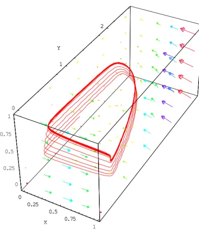
0 0.25 0.5 0.75 1 X 0 1 2 Y 0 0.25 0.5 0.75 1 Z 0 0.25 0.5 0.75 X 0 1 2 Y

Fig. 5. Phase and vectorfield portrait of the Rosenzweig-MacArthur system (26) with the same parameter values.

This figure shows slow-fast dynamic features, with long arrow for the fast features and short arrows for the slow features. This portrait consists of four branches: two fast (the shorter branches) and two slow (the longer branches). The pattern of change in this attractor resembles that of the original Volterra model. In initial, fast part of the attractor, the prey (x) rapidly increase in number, whereas the number of predators (y) and top-predators (z) remain very low. This situation realistic. Close to the equilibrium point I, the number of top-predators suddenly decreases, triggering an increase in the predator population. In the second part of the attractor, a slow stage, the number of predators increases, as does the number of top-predators, whereas the number of prey decreases. This part of the attractor leads on to another slow stage, during which the number of predators is maximal. This results in a decrease in the number of prey. In the fourth part of the attractor, a slow stage, the number of top-predators continues to increase while the number of predators decreases. As demonstrated by Deng [Deng, 2001], this attractor with a Moebius strip shape displays chaotic behaviour.

3.1.4. Slow manifold equation

Slow manifold equation based on the orthogonality principle

As described in Sec. 2.4., the slow manifold equation can be expressed as follows:

λ1Hx, y, zLzλ₁H1,β Hx, y, zL,γ Hx, y, zLL

Let us call l1(x, y, z) the fast eigenvalue of 1 (x, y, z) and zl1(1, b(x, y, z), g(x, y, z)) the fast

eigenvectors to the left of 1(x, y, z). Transposing the characteristic equation,

t_H1H

x, y, zLLz_λ1Hx, y, zL= λ1Hx, y, zLzλ₁Hx, y, zL

we can find b and g.

β = Hx+ β1L2 β1y Aλ 1− 1 ξ ikjj1−2x− 0.25yβ1 Hx+ β1L2 y { zzE γ = β 0.25y 0.25y+β₂ ∂J 0.25y 0.25y+β₂ − δ2N− λ1 x‰+ β Hx, y, zLy‰+ γ Hx, y, zLz‰=0 H27L

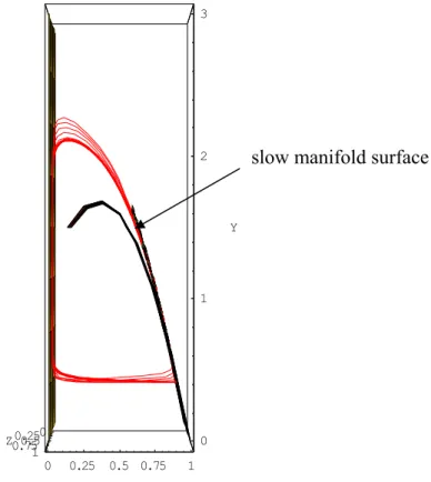
0 0.25 0.5 0.75 1 X 0 1 2 3 Y 0 0.25_0.5 0.75 1 Z

Fig. 6. Slow manifold surface defined according to the orthogonality principle. Nullcline surface corresponding to the singular perturbation and phase portrait of the Rosenzweig-MacArthur system (26), with the same parameter values. We seen here the slow manifold on which the solutions of the system (26) are based.

Slow manifold equation based on the slow eigenvectors

The slow manifold equation can be also obtained by means of the slow eigenvectors method. 3.1.5. Hopf bifurcation

We now investigate Andronov-Hopf bifurcation. The first stage of this process involves determining the parameter likely to produce such a bifurcation.

The two slow-fast parameters x and ¶ cannot generate Hopf bifurcation because they leave invariant the fixed points, they cannot cancel the real part of the eigenvalues of the functional Jacobian matrix calculated for these points. It would also appear to be most useful to consider a parameter coupling the predator-prey and predator-top-predator equations.

The parameters d1 and d2 may be involved in bifurcation. The parameter d1 has the advantage

of leaving invariant the x-co-ordinate and the y-co-ordinate of the singular point. The value of the bifurcation parameter can be calculated numerically as described in Sec. 2.3.11.

Thus, a Hopf bifurcation occurs:

- If the real part of the conjugated complex eigenvalues of the functionnal Jacobian matrix is cancelled for a certain value d1 = d1C

- If the derivative with respect to d1 of this eigenvalue calculated in d1C is non-zero

- If the other real eigenvalue evaluated in d1 is strictly negative.

The corresponding value of d1 is calculated as follows:

Re@λ2D=0

The numerical solution of this polynomial equation gives the following value:

δ1=0.683539

As the other two conditions are fullfilled, Hopf bifurcation occurs at

δ1=0.683539

Note:

The Routh & Hurwitz theorem can also be used to determine the value of the parameter d1 at

which Hopf bifurcation occurs.

Indeed, by clarifying the characteristic polynomial of the Jacobian matrix at point J, we obtain a polynomial of the form: a0+a1 λ +a2 λ2+a3 λ3 = 0.

However, according to the Routh and Hurwitz theorem, all the roots of this polynomial have negative real parts when the determinants D1, D2 and D3 are all positive.

The positivity of the first determinant D1 fullfills a condition for d1 making it possible to

3.2. The Hastings-Powell model

By changing the variables followed in the Rosenzweig-MacArthur [1963] model, we can obtain the Hastings and Powell [1991] model

dx dt =aJ1− λa xNx− b x y H1+x = x gHxL−b y pHxL dy dt =y i k jj d x H1+x − cy { zz− e y z H2+y = y@−c+d pHxLD−e z qHyL dz dt =z i k jj f y H2+y − gy { zz=z@−g+f qHyLD 3.2.1. Dimensionless equations

With the following changes of variables and parameters,

t 1 a t, x a λ x, y a d λb y, z f b a2 d eλ z dx dt =xH1−xL− a1x y 1+ β1x dy dt =y i k jj a1x 1+ β1x − δ 1y { zz− a2y z 1+ β2y H28L dz dt =z i k jj a2y 1+ β2y − δ 2y { zz with a1= d λH1 , β1= a λH1 , a2= b f dλH2 , β2= a d bλH2 ,δ1= c a,δ2= g a

By choosing a set of "biologically reasonable" parameters, system (28) becomes a singularly perturbed system of two time scales.

3.2.2. Dynamic aspects

The natural time scale of the interaction between the predator y and the super-predator z, (i.e., of interaction at the higher trophic levels), is substantially longer than that between the prey x and the predator y. In other words, d1 is much larger than d2.

Based the works of Ramdani et al. [2000], we consider the system (28) to be a slow-fast autonomous dynamic system for which we can determinate the equation of the slow manifold on which the attractor lies. A state equation binding the three variables can also be established established.

Nature and stability of the fixed points

For the initial set of values used in this simulation (x = 1, b1 = 3, b2 = 2, d1 = 0.4, d2 = 0.01,

¶

O (0, 0, 0) ö {1, -0.4, -0.01}

I (0.1052, 0.2354, 0) ö {0.00600753, 0.0547368 + 0.518656 Â, 0.0547368 - 0.518656 Â} J (0.8192, 0.125, 9.8082) ö {-0.61121, 0.038687 + 0.0748173 Â, 0.038687 - 0.0748173 Â}, K (1, 0, 0) ö {-1, 0.85, -0.01}

So according to the Lyapunov criterion, all these points are unstable.

The literal expression of the fixed points highlights their dependance on the parameters considered.

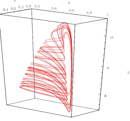
This finding will be used below, in the calculation of Hopf bifurcation. Phase portrait 0.2 0.4 0.6 0.8 1 X 0.1 0.2 0.3 0.4 Y 8 9 10 Z 0.1 0.2 8 9

3.2.3. Slow manifold equation

Slow manifold equation based on the orthogonality principle

As describe in Sec. 2.4., the equation of the slow manifold can be expressed as follows:

λ1Hx, y, zLzλ₁H1,β Hx, y, zL,γ Hx, y, zLL

Let us call l1(x, y, z) the fast eigenvalue of 1 (x, y, z) and zl1(1, b(x, y, z), g(x, y, z)) the fast

eigenvectors to the left of 1(x, y, z). Transposing the characteristic equation,

t_H1H

x, y, zLLz_λ1Hx, y, zL= λ1Hx, y, zLzλ₁Hx, y, zL

we can find b and g.

β =i k jj H1+xβ1L2 5y y { zzi k jjλ1−H1−2xL+ 5 y H1+xβ1L2 y { zz γ = β 0.1y 0.1y−H1+yβ2LHδ2+ λ1L

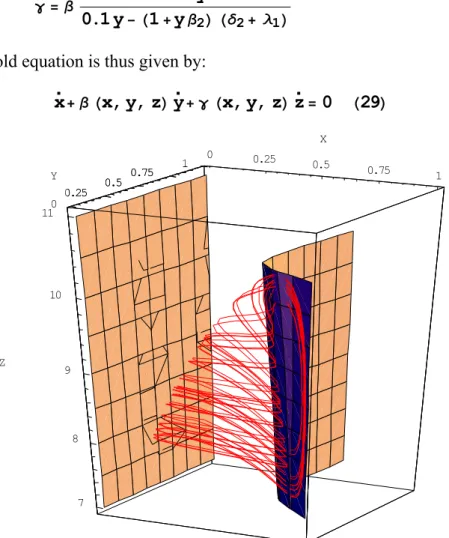
The slow manifold equation is thus given by:

x‰+ β Hx, y, zLy‰+ γ Hx, y, zLz‰=0 H29L 0 _0.25 0.5 _0.75 1 X 0 0.25 0.5 0.75 1 Y 7 8 9 10 11 Z 0.25 0.5 0.75 1

Fig. 8. Slow manifold surface based on the orthogonality principle and phase portrait of the Hastings and Powell system (28) with the same parameter values.

3.2.4. Hopf bifurcation

We will now focus on Andronov-Hopf bifurcation. The first stage in this process involves identifying the parameter likely to produce such a bifurcation.

The slow-fast parameters x and ¶ cannot generate bifurcation as they leave the fixed points invariant and they cannot cancel the real part of the eigenvalues of the functionnal Jacobian matrix calculated for these points. It would also be useful to consider a parameter coupling the two predator-prey and predator- top-predator equations.

The parameters d1 and d2 may also be considered. The parameter d1 has the advantage of

leaving invariant the x-co-ordinate and the y-co-ordinate of the singular point. It also modifies the topology of the attractor, conferring on it the Moebius strip shape of the Rosenzweig-MacArthur model at a certain value .

We can therefore fix all the values of the parameters at the levels described above, except for d1. The technique described in Sec. 2.3.11. can then be used for numerical calculation of the

bifurcation parameter value. Thus, Hopf bifurcation occurs:

- If the real part of the complex conjugated eigenvalues of the functional Jacobian matrix is cancelled for a certain value d1 = d1C

- If the derivative with respect to d1 of this eigenvalue calculated in d1C is non-zero

- If the other real eigenvalue evaluated in d1 is strictly negative.

The corresponding value of d1 is calculated as follows:

Re@λ2D=0

The numerical solution of this polynomial equation gives the following value:

δ1=0.7402

As the other two conditions are fullfilled, the Hopf bifurcation occurs at

δ1=0.7402

In addition, by selecting b1 as the bifurcation parameter and proceeding as describe above, it

is possible to calculate the value of this parameter with a high degree of precision. Indeed, cancelling the part of the complex eigenvalues of the functional jacobian matrix evaluated at the fixed point I according to the parameter b1 generates the value: b1 = 2.11379.

3.3. Similarity between the various models

The Volterra-Gause model, as described above, directly resembles the Rosenzweig-MacArthur model for certain parameter values.

Indeed, these two models present similar dynamic behaviour (Fig. 9). Below the bifurcation threshold, we find the overall shape of the chaotic attractor of the Rosenzweig-MacArthur model. 0 0.25 0.5 0.75 1 X 0 1 2 Y 0.25 0.5 0.75 1 Z 0 0.25 0.5 0.75 X 1 2 Y

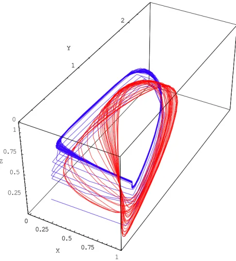
Fig. 9. Comparison of the Volterra-Gause model (for x = 0.964, ¶ = 1.1, d1 = 0.518,

d2 = 0.415) and the Rosenzweig-MacArthur model (for x = 0.1, b1 = 0.3, b2 = 0.1, d1 = 0.1,

3.3.2. The Volterra-Gause and Hastings-Powell models

The similarity between the Volterra-Gause model and the Hastings and Powell model, with its famous "up-side-down teacup" is more striking. The followings figures show the basic teacup shape and the behaviour of each component x, y, z over time.

0.2 0.4 0.6 0.8 x 0.5 1 1.5 y 0.2 0.4 0.6 0.8 1 z

Fig. 10. Phase portrait of the Volterra-Gause model (for x = 0.07, ¶ = 0.85, d1 = 0.5,

700 800 900 1000 t 0.2 0.4 0.6 0.8 1 1.2 1.4 x 200 400 600 800 1000 t 0.2 0.4 0.6 0.8 1 1.2 1.4 x

Fig. 11. Comparison of the changes over time in the Volterra-Gause (for x = 0.07, ¶ = 0.85, d1 = 0.5, d2 = 0.42 ) and Hastings-Powell models (for ξ =1, b1 = 3, b2 = 2, d1 = 0.4, d2 = 0.01,

3.3.3. The Rosenzweig-MacArthur and Hastings-Powell models

The bifurcation parameter d1 chosen in Sec. 2.1.5. modifies the topology of the attractor of the

Rosenzweig-MacArthur model conferring on it, at a certain value, the shape of the so-called "up-side-down tea-cup" of the Hastings and Powell [1991] model.

We can therefore fix all the parameters at values cited above, except for d1. Varying the

parameter d1 up to a value of 0.3, preserves a limit cycle, which becomes deformed, resulting

in a passage from the Rosenzweig-MacArthur model to the Hastings and Powell model.

0 0.25 0.5 0.75 1 X 0 0.5 1 1.5 2 Y 0 0.2 0.4 0.6 0.8 Z

Fig. 12. Transition from the Rosenzweig-MacArthur model to the Hastings and Powell [1991] model

In this figure, we can identify the attractor in the shape of a teacup, for the Hastings and Powell [1991] model with d1 = 0.3.

3.3.4. The Hastings-Powell and Rosenzweig-MacArthur

The Hastings-Powell model can also be converted to the Rosenzweig-MacArthur model.. Varying the bifurcation parameter d1 modifies the topology of the attractor, conferring on it

the Moebius strip shape of the Rosenzweig-MacArthur model at a certain value. We can therefore fix all the parameters at the values cited above, except for d1.

Variation of the parameter d1 up to a value of 0.1, results in a passage from the model of

Hastings and Powell to the of Rosenzweig-MacArthur model.

0 0.25 0.5 0.75 1 x 0 0.5 1 1.5 y 7 8 9 10 11 z 0 0.25 0.5 0.75 x

Fig. 13. Transition from the Hastings and Powell model to Rosenzweig-MacArthur model. On this figure, we can see the attractor with the Moebius strip shape of Rosenzweig-MacArthur model at d1 = 0.1.

4. Discussion

In this work, we have shown certain similarities between the three models considered.

The common features of these models, the possibility of transition from one model to another by parameter variation and the differences between these models provide biologists with alternatives in their choice of predator-prey model.

Despite differences in their functional responses, these models present striking similarities in the nature and number of their fixed points, and in their dynamic behaviour: existence of a limit cycle, occurrence of Hopf bifurcation, presence of a chaotic attractor or period doubling cascades.

Dynamical features \ Models Rosenzweig-MacArthur Hastings- Powell Volterra- Gause Equilibriumpoints OH0, 0, 0L IHx `<sub>, y`, 0L</sub> JHx*, y*, z*L KH1, 0, 0L OH0, 0, 0L IHx`, y`, 0L JHx*, y*, z*L KH1, 0, 0L OH0, 0, 0L IHx`, y`, 0L JHx*, y*, z*L KH1, 0, 0L Attractional sink 2 2 2 Hopf bifurcation d1= 0.6835 d1= 0.7402 d1= 0.7474

Chaoticattractor Moebius strip Teacup Snail shell Period-doubling d2= 0.67785 b1= 2.437 d1= 0.625

Slowmanifold 1 1 1

The fixed point O (0, 0, 0) presents the same stability in all three models, with attractive eigendirections according to z'z and repulsive eigendirections according to x'x. The eigendirections of point K (1, 0, 0) are attractive according to x'x and z'z in all three models. Points I(xˆ,yˆ,0) and J (x*, y*, z*) behave as a stable and an unstable focus, respectively, with I in the xy plane and J apart from the xy plane. These models introduce rich and complex dynamics, for which further study is required.

It also appears to be possible, in some domains of parameter variation, to reduce the the dimension of the models, making it possible to take into account the influence of the external medium by means of time-dependent coefficients.

Acknowledgements

Certain numerical results and graphs were not possible without the use of powerful programs designed by Eric Javoy.

References

Deng, B. [2001] "Food chain chaos due to junction-fold point," Am. Inst. of Physics 11 (3), 514-525.

Freedman, H.I. & Waltman, P. [1977] "Mathematical analysis of some three-species food-chain models, " Mathematical Biosciences 33, 257-276.

Gause, G.F. [1935] The struggle for existence (Williams and Wilkins, Baltimore)

Glass, L. & Mackey, M.M. [1988] From clocks to chaos (Princeton University Press, Princeton, New Jersey, USA).

Hastings, A. & Powell, T. [1991] "Chaos in a three-species food chain," Ecology 72, 896-903. Holling, C.S. [1959] "Some characteristics of simple types of predation and parasitism," Can. Entomologist 91, 385-398.

Kuznetsov, Y. [1995] Elements of Applied Bifurcation Theory (Springer & Verlag, New York).

Lotka, A.J. [1925] Elements of Physical Biology (Williams and Wilkins, Baltimore).

Muratori, S. & Rinaldi, S. [1992] "Low and high frequency oscillations in three dimensional food chain systems," SIAM J. Appl. Math. 52, 1688-1706.

Ramdani, S., Rossetto, B., Chua, L. & Lozi R. [2000] "Slow Manifold of Some Chaotic Systems-Laser Systems Applications," Int. J. Bifurcations and Chaos 10, Vol.12, 2729-2744. Rinaldi, S. & Muratori, S. [1992] "Slow-fast limit cycles in predator-prey models," Ecological Modelling 61, 287-308.

Rosenzweig, M.L. & Mac Arthur, R.H. [1963] "Graphical representation and stability conditions of predator-prey interactions," Am. Nat. 97, 209-223.

Rosenzweig, M.L. [1971] "Paradox of enrichment : destabilisation of exploitation ecosystems in ecological time," Science 171, 385-387.

Verhulst, P.F. [1838] "Notice sur la loi que suit la population dans son accroissement," Corresp. Math. Phys. X, 113-121 [in French].

Volterra, V. [1926] "Variazioni e fluttuazioni del numero d'individui in specie animali conviventi," Mem. Acad. Lincei III 6, 31-113 [in Italian].