Aerodynamic study of a 3D backward facing double step applied to safer launch and recovery of helicopters on ships

(1)

HAL Id: tel-00650410

https://tel.archives-ouvertes.fr/tel-00650410

Submitted on 10 Dec 2011

HAL is a multi-disciplinary open access

archive for the deposit and dissemination of sci-entific research documents, whether they are pub-lished or not. The documents may come from teaching and research institutions in France or abroad, or from public or private research centers.

L’archive ouverte pluridisciplinaire HAL, est destinée au dépôt et à la diffusion de documents scientifiques de niveau recherche, publiés ou non, émanant des établissements d’enseignement et de recherche français ou étrangers, des laboratoires publics ou privés.

Aerodynamic study of a 3D backward facing double step

applied to safer launch and recovery of helicopters on

ships

Benjamin Herry

To cite this version:

Benjamin Herry. Aerodynamic study of a 3D backward facing double step applied to safer launch and recovery of helicopters on ships. Fluid mechanics [physics.class-ph]. Université de Valenciennes et du Hainaut-Cambresis, 2010. English. �NNT : 10/47�. �tel-00650410�

(2)

N◦ d’ordre : 10/47

Université de Valenciennes et du Hainaut Cambrésis École Doctorale Sciences Pour l’Ingénieur Université Lille Nord-de-France

THÈSE DE DOCTORAT présentée pour obtenir le titre de DOCTEUR

Spécialité : Mécanique Par

Benjamin HERRY

ÉTUDE AÉRODYNAMIQUE D’UNE DOUBLE MARCHE DESCENDANTE 3D APPLIQUÉE A LA SÉCURISATION DE L’APPONTAGE DES

HÉLICOPTÈRES SUR LES FRÉGATES

Soutenue publiquement le 20 décembre 2010 devant le jury composé de:

PRÉSIDENT

Gérard BOIS Professeur, Université de Lille

RAPPORTEURS

Jean-Yves BILLARD Professeur, Université de Brest

Azeddine KOURTA Professeur, Université d’Orléans EXAMINATEURS

Grégory COUSSEMENT Professeur, Université de Mons

Éric GARNIER HDR, ONÉRAMeudon

Larbi LABRAGA Professeur, Université de Valenciennes, Directeur de thèse

Laurent KEIRSBULCK Maître de conférences, Université de Valenciennes, Co-encadrant

Bruno MIALON Ingénieur, ONÉRALille

INVITÉS

Jean-Bernard PAQUET Docteur Ingénieur, ONÉRALille, Co-encadrant

(3)

(4)

“Was mich nicht umbringt, macht mich stärker.”

(5)

(6)

Acknowledgements

Cette page est probablement la plus difficile de toutes à écrire. Il n’y a pourtant pas de calculs à faire. Au contraire, il s’agit d’exprimer avec sincérité la gratitude et la recon-naissance envers ceux qui ont marqué de prés et/ou de loin ces trois dernières années passées à l’Onera de Lille.

Sans remonter à la genése pour remercier toutes les raisons qui ont conduit à mon ex-istence et mes conditions de vie, une pensée légitime devrait cependant au moins être attribuée à mes proches. Contrairement à beaucoup d’autres auteurs, ce ne sera pas fait ici: une page (aux bas mots) leur est en effet déjà dédiée . . .

En revanche, un hommage doit être rendu à l’Onera qui a permis de remplir sans pri-vation un grand réfrigérateur, notamment d’une petite collection à déguster de bières du Noooooord. Mais plus que l’institution, ce sont les hommes qui ont laissé leurs em-preintes. Tout d’abord, Bruno Mialon, chef d’unité, qui a toujours fait son maximum pour qu’avancent les choses et en particulier pour que soient réglées au mieux les dif-ficultés bassement matérielles. Dans son rôle de manager de personnel, ce fut lui qui apporta aussi (peut-être à son insu d’ailleurs!) la reconnaissance tant attendue dans l’inévitable moment de solitude et de perte de confiance que vivent certains doctor-ants. . . . Mon “plus que collègue maintenant”, François Touron sait de quoi il s’agit, lui qui prenait les relais au mégaphone pour le ’Rame!’ (ter repetitam). Le relai passe dé-sormais dans les mains de mes amis, Thomas et Stéphane de MMHD, qui auront rempli cette dernière année de mémorables cartons jaunes et rouges. Bon courage et réussite à eux. Bonne continuation aussi à ceux qui ont apporté leur aide . . . toute l’équipe MMHD en fait! Certains gardent une place particulière dans ma mémoire; ils se recon-naitront.

Finalement, ces trois années ont étés très riches en enseignement et pas uniquement sur le plan scientifique, loin s’en faut. Je remercierai à cet égard les encadrants de cette thèse, Larbi Labraga, Laurent Keirsbulck et Jean-Bernard Paquet, qui ont partagé bien plus que leurs connaissances, puiqu’ils m’ont accordé leur confiance en me laissant par là même une grande autonomie.

Enfin, le ruban entourant ce mémoire ne pourrait jamais être noué sans les membres du jury. A cet égard, le rôle des rapporteurs est irremplaçable et bien entendu, j’exprime toute ma reconnaissance aux professeurs Jean-Yves Billard et Azeddine Kourta qui ont accepté cette tâche de relecture, parfois ingrate. Je remercie aussi Eric Garnier ainsi que les professeurs Gérard Bois et Grégory Coussement dans leur rôle d’examinateurs. En-fin, c’est un plaisir de revoir Joop Gooden au delà de la coopération Onera/NLR, et de pouvoir discuter à nouveau avec lui en toute modestie.

Cette liste de remerciements n’est bien sûr pas exhaustive, mais les absents savent qu’ils n’ont pas étés oubliés.

(7)

(8)

Résumé détaillé

Cette étude s’inscrit dans le domaine de la sécurisation de l’appontage des hélicoptères sur les frégates. En effet, cette phase d’une mission d’un pilote d’hélicoptère est l’une des plus difficile et dangereuse qui soit, principalement du fait de la forte charge de tra-vail qu’il subit. Les principales causes résident dans les mouvements de plateformes et l’aérodynamique défavorable au dessus des ponts d’envol. Le problème étant com-plexe, il doit être simplifié. En particulier, l’impact du sillage aérodynamique de la frégate sur le vol de l’hélicoptère doit être isolé. Sachant que les taux de turbulence les plus élevés induisant une charge de travail maximum sur les pilotes sont rencon-trés lorsque le vent relatif est fort et qu’il est dans l’axe du bateau, il s’agit d’analyser ce type d’écoulement à dérapage nul du navire, sans mouvement et sans hélicoptère. Une étude bibliographique a permis de montrer qu’il existait déjà des travaux sur la modélisation de sillages aérodynamiques de frégates. En particulier, des géométries génériques ont été définies sur lesquelles des essais expérimentaux ainsi que des cal-culs numériques ont été réalisés. Ces premiers travaux ont permis de donner une pre-mière description de la topologie de l’écoulement moyen au dessus de la plateforme d’appontage. Sur une configuration géométrique particulière (mais symétrique), deux auteurs observent à la fois expérimentalement et numériquement un phénomène inat-tendu d’asymétrie de l’écoulement moyen à angle de dérapage nul. Toutefois, il n’est ni décrit, ni expliqué. D’autre part, les travaux s’attardant sur la phénoménologie insta-tionnaire de l’écoulement sont très peu nombreuses alors que cet aspect est fondamen-tal pour la problématique de l’appontage. Ainsi, afin de mieux comprendre ces carac-téristiques qui ne sont pas abondamment décrites dans la littérature, une démarche a été entreprise afin d’isoler l’écoulement au dessus de la plateforme, de le sonder et d’en étudier en particulier l’asymétrie de l’écoulement moyen ainsi que ses conséquences éventuelles sur la problématique de l’appontage.

Cette démarche a d’abord consisté à définir une version améliorée de géométrie générique de frégate décrite dans la littérature afin d’obtenir en amont du hangar des condi-tions les plus uniformes possibles. Ceci conduit à modéliser le bateau par une dou-ble marche descendante 3D avec un nez en forme d’ogive. La forme est choisie afin que des couches limites de type plaque plane se développent sur les quatre faces de la maquette et donc d’obtenir en amont de la première marche (modélisant le hangar, de hauteur h) des couche limites canoniques. Ceci est aussi permis en plaçant la maquette au bord d’attaque d’une table de 49h de long, ce qui a pour effet d’extraire le maque-tte de la couche limite se développant sur le sol de la soufflerie, mais aussi créant un

(9)

Résumé détaillé viii espace libre permettant à l’air de librement circuler entre la maquette et le sol souf-flerie. L’ensemble table/maquette est alors monté dans la soufflerie subsonique du laboratoire TEMPO de Valenciennes, disposant d’une veine d’essai de 2 × 2 × 10 m3_.

Cette soufflerie est choisie pour son faible taux de turbulence et ses grandes dimen-sions permettant d’atteindre des nombres de Reynolds élevés, supérieurs à 8.75 × 104

(basés sur la hauteur de marche et la vitesse amont de l’écoulement libre). Ces hauts nombres de Reynolds sont nécessaires afin que les couches limites qui se développent en amont de la première marche soient turbulentes établies, permettant d’obtenir un régime représentatif de l’écoulement à l’échelle 1. Cette caractéristique d’écoulement turbulent est vérifiée en sondant le profil d’une des couches limites latérales en amont de la première marche. L’uniformité de l’écoulement amont est qualitativement véri-fiée par des visualisations par enduit gras et tomoscopie laser.

L’écoulement en amont de la première marche étant caractérisé, l’attention est alors portée sur l’écoulement en son aval. Pour cela, de l’enduit gras est utilisé pour tracer les lignes de frottement pariétales moyennes : les empreintes d’un tourbillon en U in-versé apparaissent avec une très légère asymétrie. De plus, la longueur de rattachement est estimée à 2,8h. Cette valeur est alors confirmée par PIV dans le plan de symétrie en localisant la position du point de vitesse longitudinale nulle en moyenne. Ce cliché met en évidence une zone de recirculation primaire et secondaire, tout comme en aval d’une marche 2D. Le tourbillon en U inversé est cependant mieux visualisé dans le plan PIV horizontal, réalisé à mi-hauteur de marche : les lignes de courant montrent alors une forte asymétrie de l’écoulement moyen dans ce plan. Une explication de ce phénomène est alors recherchée dans l’analyse de l’écoulement instationnaire.

Les fluctuations d’écoulement sont décrites et une analyse POD est entreprise à partir des données des 2 plans PIV. Le premier mode du plan de symétrie de la maquette semble traduire un phénomène de battement de la couche de cisaillement, ce que les mesures de corrélations croisées corroborent. Les modes suivants, quant à eux, sem-blent plus rapportés à un phénomène de lâchers tourbillonnaires dans la couche de cisaillement. En revanche, dans le plan à mi-hauteur de marche, les premiers modes ne traduisent a priori pas de phénomène instationnaire académique. Les modes dans ce plan sont asymétriques, traduisant l’asymétrie de l’écoulement fluctuant à dérapage nul malgré une géométrie symétrique. Pour mieux comprendre la phénoménologie instationnaire de cet écoulement, un spectre est obtenu de part et d’autre du plan de symétrie, en aval de la première marche. Un pic net apparait pour un Strouhal de 0,08 (basé sur la hauteur de marche et la vitesse infinie amont). Une forte contribution des plus basses fréquences est aussi bien visible, sans cependant noter de pic étroit. De la to-moscopie laser haute cadence est alors réalisée afin de tenter d’associer une fréquence à un phénomène aérodynamique particulier. L’approche n’est pas parfaitement con-cluante. Elle permet cependant d’estimer et de confronter les mesures par fil chaud

(10)

Résumé détaillé ix de la vitesse d’advection des structures cohérentes, montrant une accélération de ces dernières lors de leur éloignement de la marche. Leur trajectoire est enfin déterminée par une analyse statistique utilisant le critère de détection . Cette approche requiert cependant un approfondissement afin de mieux comprendre la phénoménologie 3D instationnaire de cet écoulement.

Une des originalités principales de cette étude réside toutefois dans l’élaboration d’un protocole expérimental visant à mettre en évidence des cas d’apparition de cette asymétrie de l’écoulement moyen. Le premier paramètre étudié est l’angle de dérapage. La très grande sensibilité de l’écoulement moyen avec ce paramètre est observée par PIV dans le plan à mi-hauteur de marche. L’écoulement moyen symétrique n’est d’ailleurs pas obtenu. Les conditions amont à la marche sont alors modifiées pour voir si elles ont une quelconque influence sur le résultat. Tout d’abord, la maquette est posée au sol d’une autre soufflerie (Onera L2) ayant la propriété de simuler une couche limite at-mosphérique marine et donc de présenter des taux de turbulence élevés (jusqu’à 7% en proche paroi). Dans cette soufflerie, des visualisations par tomoscopie laser dans le plan à mi-hauteur de marche ainsi que des mesures de pression pariétales sont réal-isées. Aucune influence de ce changement des conditions amont sur l’écoulement moyen n’est observée. Le résultat est le même lorsque le nez des maquettes est modifié, contrôlant ainsi l’état attaché ou détaché des couches limites supérieure et latérales en amont de la première marche. L’ajout d’un parallélépipède (modélisant une cheminée) sur la face supérieure de la maquette n’a pas non plus d’influence sur le résultat. La propriété d’asymétrie de l’écoulement moyen semble donc peu influencée par les con-ditions amont à la maquette. Pour vérifier cette hypothèse, une simulation numérique est conduite sur un domaine fluide débutant en aval du nez, annulant ainsi l’influence de ce dernier. L’angle de dérapage géométrique est nul et les conditions amont sont mathématiquement uniformes. Malgré cela, le modèle RANS stationnaire de Spalart-Almaras prédit un écoulement asymétrique en moyenne. Les coefficients de pression correspondent d’ailleurs bien avec les valeurs expérimentales. En plus de donner une idée de la topologie 3D de l’écoulement, ce calcul semble mettre en évidence l’absence d’influence des conditions amont sur l’écoulement moyen autour de telles géométries dans le domaine de conditions testées. Mais est-ce valable pour toutes conditions? Sachant que le nombre de Reynolds peut-être un paramètre critique conditionnant ou non de tels phénomènes, un troisième montage est réalisé utilisant une maquette de petite taille conduisant à un nombre de Reynolds de 5.9 × 103 _{(basé sur la hauteur}

de marche). L’écoulement en amont de la marche est donc attendu laminaire et pour-tant, l’asymétrie en aval est toujours visualisée par tomoscopie laser. Pour l’ensemble de valeurs étudiées, le nombre de Reynolds n’est donc pas un paramètre influençant cette asymétrie de l’écoulement moyen. Il reste cependant à expliquer ce phénomène d’asymétrie. Pour cela, les clichés instantanés PIV et tomoscopie laser sont analysés

(11)

Résumé détaillé x individuellement. Ils peuvent être rangés en deux familles distinctes, l’une présen-tant un gros tourbillon d’un côté de la maquette, et l’autre éprésen-tant son symétrique. Il est montré que les clichés d’une même famille se succèdent, laissant place à un ensemble de clichés de l’autre famille. Ceci suggère donc l’existence de deux solutions stables de l’écoulement et laissent penser que la solution moyenne symétrique est instable. La bascule d’une solution à l’autre est aléatoire à angle de dérapage nul avec, a pri-ori, équiprobabilité d’apparition des deux solutions. En revanche, lorsque l’angle de dérapage devient non nul, une solution apparait plus souvent que l’autre : l’asymétrie de l’écoulement moyen est donc un effet de moyenne dû à cette caractéristique de la bi-stabilité de l’écoulement. Ce phénomène est-il toutefois important pour la problé-matique de l’appontage ?

Une première approche considérant quelques critères de la littérature laisse penser que le phénomène de bascule d’une solution à l’autre risque d’avoir des conséquences néfastes sur l’appontage des hélicoptères. De ce fait, une modélisation fidèle de ce phénomène peut s’avérer nécessaire. Pour cela, des travaux complémentaires sur la compréhension de l’écoulement 3D instationnaire ne semblent pas inutiles. Compren-dre les origines du phénomène de bi-stabilité serait aussi d’une grande aide pour son éventuel contrôle. Cependant, avant cela, une hypothèse forte qui avait été faite pour cette étude doit être vérifiée : l’approche considérant négligeable l’influence du sillage rotor sur l’écoulement est-elle valable ? Si cela justifie l’étude du sillage aérodynamique seul en absence de rotor, ce la bonne approche ? Le phénomène de bi-stabilité est-il toujours présent lorsqu’un rotor d’hélicoptère se trouve au dessus de la plateforme ? Une étude paramétrique devrait être réalisée afin de déterminer pour quelles carac-téristiques de triplet hélicoptères/frégates/conditions de vent l’hypothèse précédente est valable. Le sujet est donc encore loin d’être clos.

(12)

List of Figures

1.1 Flow topology downstream of a 2D backward facing step flow . . . 6

1.2 Apparition of several secondary vortices for low aspect ratio steps . . . 7

1.3 Dependence of the reattachment length with the upstream boundary layer state . . . 8

1.4 Dependence of the reattachment length on the upstream boundary layer thickness . . . 9

1.5 Dependence of the reattachment length on the expansion ratio . . . 9

1.6 Some vortex detection using the Q criterion . . . 12

1.7 Vortex shedding characteristics downstream of a cylinder . . . 13

1.8 Streamlines of the time-averaged fow around rectangular cylinders with different aspect ratios . . . 14

1.9 Flow topology around a wall-mounted cube . . . 18

1.10 Interpreting the 3D shape of a vortex through 2D measurements . . . 19

1.11 Von Karman street materialized by clouds downstream of Alexander Selkirk island in the southern Pacific ocean . . . 22

1.12 The effect of building geometry on vortex-shedding frequency in turbu-lent flow . . . 23

1.13 Several Simplified Frigate Shapes found in the literature . . . 25

1.14 Surface streaklines of the 1ststep of the SFS1: (a) experimental, (b) com-putation . . . 26

1.15 Mean and RMS streamwise velocities across the backward cuboid of the SFS2, in the vertical plane located at 1.1h downstream of the first step and at step height . . . 27

1.16 Perspective view of the flow downstream of the SFST . . . 29

1.17 Some features of the flow in x planes of the SFST . . . 30

2.1 Coordinate system and definition of the geometric drift angle . . . 32

2.2 SFSO’: alone and on its table . . . 33

2.3 The TEMPO wind tunnel of Valenciennes . . . 34

2.4 Positioning of the hot wire probes for mean advection velocity measure-ments . . . 38

2.5 Positions of the hot-wire probes for spectra measurements and advection velocity determination . . . 39

2.6 PIV camera positioning in plane y0= 0 . . . 42

2.7 PIV camera positioning in the z planes . . . 43

2.8 The two positions of the perturbators on the SFSs . . . 45

2.9 Definition of the short SFS1’ . . . 45

2.10 The L2 wind tunnel . . . 46 xvii

(19)

List of Figures xviii

2.11 Smoke injection for the laser tomoscopy visualizations . . . 47

2.12 Position of the camera for laser tomoscopy visualizations . . . 47

2.13 Position of the pressure taps . . . 49

2.14 The L2 wind tunnel simulated atmospheric boundary layer . . . 50

2.15 The mini wind tunnel . . . 51

2.16 Probing the mini wind tunnel . . . 52

2.17 The computing domain and the structured mesh . . . 54

2.18 Evolution of the residuals against the number of iterations performed . . 55

3.1 Oil visualizations over the central cuboid of the SFSO’ . . . 59

3.2 Flow visualization in the plane x/h = −0.13 . . . 60

3.3 Surface oil flow visualization on the top surface of the backward cuboid 62 3.4 Streamlines and streamwise and spanwise velocity contour levels in the high resolution y0 = 0plane at Reh= 8 × 104 . . . 63

3.5 Determining the reattachment length behind the first step Reh= 8 × 104 64 3.6 Streamlines and velocity contour levels in the plane z/h = 0.784, Reh = 9.75 × 104. . . 65

3.7 Streamlines and velocity contour levels in the plane z/h = 0.5, Reh = 9.75 × 104. . . 66

3.8 Estimated Position of the z planes relative to the estimated arch vortex shape . . . 66

3.9 3D view of the arch vortex . . . 67

3.10 Turbulence intensity and turbulence production in the plane Y = 0, Reh = 9.75 × 104 . . . 68

3.11 Forward and upward flow intermittency factors in the plane y = 0 at Reh = 8 × 104 . . . 69

3.12 Evolution of the mean streamwise velocity and the forward flow inter-mittency factor . . . 70

3.13 POD energy of the modes and sum of the mode energy . . . 70

3.14 Streamlines and longitudinal velocity contour levels of the first 4 POD modes in the plane y = 0 at Reh = 9.75 × 104 . . . 71

3.15 Estimated values of Skewness and kurtosis in the plane y = 0 at Reh = 9.75 × 104. . . 72

3.16 Illustration of the positions where the skewness, kurtosis and PDF are extracted in the plane y = 0 . . . 73

3.17 Estimated probability density functions compared to the normal distri-bution at different locations in the plane y = 0 at Reh= 9.75 × 104 . . . . 74

3.18 Turbulence intensities and turbulence production in the plane z/h = 0.5, Reh = 9.75 × 104 . . . 76

3.19 Mean (solid) and RMS (dashed) streamwise velocities along the line (x/h, z/h) = (1.12, 0.814) . . . 76

3.20 Forward and sideways flow intermittency factors in the plane z/h = 0.5 at Reh= 9.75 × 104 . . . 77

3.21 Streamlines and longitudinal velocity contour levels of the first 4 POD modes in the plane z/h = 0.5 at Reh = 9.75 × 104 . . . 77

3.22 Estimated values of Skewness and kurtosis in the plane z = 0.5 at Reh= 9.75 × 104. . . 78

(20)

List of Figures xix 3.23 Illustration of the positions where the skewness, kurtosis and PDF are

extracted in the plane z/h = 0.5 . . . 79 3.24 Estimated probability density functions compared to the normal

distri-bution at different locations in the plane z/h = 0.5 at Reh= 9.75 × 104 . 80

3.25 Illustration of the positions where the spectra were computed, in the vicinity of the plane z/h = 0.5 . . . 81 3.26 Normalized spectra at positions 2 : (x/h, y/h, z/h) = (2.37, −0.61, 0.53)

and 1 : (x/h, y/h, z/h) = (2.34, 0.58, 0.45) for Reh = 1.675 × 105 . . . 81

3.27 Time evolution of streamwise vortices in the plane x/h = 1.6 at Reh =

9.75 × 104. . . 83 3.28 Time evolution of shear layer smoke puffs in the plane y/h = 0 at Reh=

9.75 × 104. . . 84 3.29 Time evolution of shear layer smoke puffs in the plane z/h = 0.47 at

Reh = 9.75 × 104 . . . 85

3.30 Time evolution of shear layer smoke puffs in the plane z/h = 0.47 at Reh = 1.65 × 105 . . . 86

3.31 Spatial turbulence integral length scales in the plane y = 0.5 at Reh =

9.75 × 104. . . 88 3.32 Spatial turbulence integral length scales in the plane z/h = 0.5 at Reh =

9.75 × 104. . . 88 3.33 Streamwise autocorrelation coefficient along the x and the z axis in the

plane y = 0.5 at Reh = 9.75 × 104 . . . 89

3.34 Coherent structures detection in the planes y = 0 and z/h = 0.5 at Reh=

9.75 × 104using the Γ1criterion . . . 91

3.35 . . . 92 3.36 . . . 93 3.37 Mean advection velocity of the coherent structures in different positions

behind the first step at Reynolds number Reh = 9.75 × 104 and Reh =

1.65 × 105and illustration of the positions probed . . . 94 4.1 Surface oil flow visualization on the top surface of the backward cuboid

at βg = 0.21◦ . . . 98

4.2 PIV on the SFSO’ in the z/h = 0.5 plane: evolution against the drift angle of streamlines and iso-contour of U/U0 without and with the hysteresis

test. Reh= 9.75 × 104 . . . 100

4.3 SFSC’: flow is detached on the upper wall and attached on the lateral walls104 4.4 Attached flow on the upper and sidewalls of the SFSO’ . . . 104 4.5 Effect on the upper boundary layer of the cylinder placed upstream of

the first step at (a) x/D = −10 and (b) x/D = −2 . . . 104 4.6 ∆Cp = Cpy>0− Cpy<0against βaat position (x/h, z/h) = (−5.88, 0.5) at

Reh = 1.8 × 105for the SFSO’, SFSC’ and SFS1’ . . . 106

4.7 Representative snapshot of the flow in the z/h = 0.5 plane when the mean flow asymmetry is observed . . . 107 4.8 Maps of pressure coefficients over the top surface of the SFSO’ backward

cuboid at several drift angles . . . 108 4.9 Maps of pressure coefficients over the top surface of the SFSC’ backward

cuboid at several drift angles . . . 109 4.10 Maps of pressure coefficients over the top surface of the SFS1’ backward

(21)

List of Figures xx 4.11 Observing the mean flow asymmetry using CFD at Reh= 4.9 × 105 . . . 111

4.12 Observing the mean flow asymmetry using CFD. 3D streamlines and friction velocity contours at the surface . . . 112 4.13 Comparison of the ∆Cp = Cpy>0 − Cpy<0 obtained through CFD and

experiments on the SFSC’ and SFSO’ at positive drift angle . . . 113 4.14 Visualization of the y < 0 streamwise vortex through 3D streamlines. In

color: normalized friction velocity contours levels . . . 114 4.15 Cp coefficients in the z/h = 0.02 plane . . . 115 4.16 A representative snapshot from laser tomoscopy in the z/h = 0.5 plane

of the SFSC’ at Reh = 5.9 × 103 . . . 116

4.17 Velocity streamlines and contour levels on a representative PIV snapshot 117 4.18 The 2 control contours C1and C2for the computation of the circulation . 117

4.19 An average field A decomposed as the weighted sum of solutions A1

and A2. Here, α = 33% and βa= 0.04◦ . . . 118

4.20 Proportion of type I snapshots against βafor the PIV measurements on

the SFSO’ at Reh= 9.75 × 104and the tomoscopy snapshots on the SFSC’

at Reh= 5.9 × 103 . . . 118

4.21 Inclined splitter plate behind the second step of the SFSC’ at Reh = 5.9×103121

4.22 Some control devices put on the SFSC’ to test the influence of the stream-wise vortices on the bi-stability at Reh= 5.9 × 103 . . . 122

4.23 Control device on the lateral wall, upstream of the first step of the SFSC’ at Reh= 5.9 × 103 . . . 122

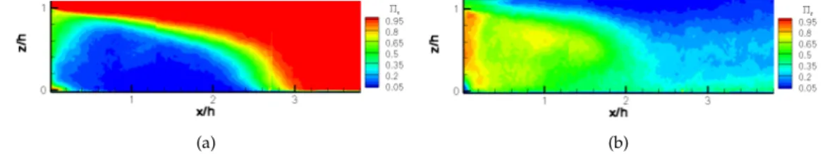
5.1 FREMM: the next generation frigate of the French Navy with its helicopter128 5.2 Change in mean velocity in the plane z/h = 0.5 at Reh = 9.75 × 104

resulting from the flow flip-flopping . . . 129 5.3 2D streamlines and contour levels of the normalized streamwise velocity

in the plane z/h = 0.5 at βg = 8.7◦ . . . 133

(22)

List of Tables

2.1 Oil visualization test program . . . 36 2.2 Laser tomoscopy visualization test program . . . 37 2.3 Hot-wire test program . . . 40 2.4 PIV test program . . . 41 2.5 Upstream conditions imposed at the entry of the computational domain 54 3.1 Some features at the surface of the flow behind the first step . . . 61 3.2 Characteristics of the recirculation bubbles behind both steps . . . 64 3.3 Characteristics of the vortices in the plane z/h = 0.5 . . . 66 3.4 Skewness and kurtosis at some locations in the plane y = 0 at Reh =

9.75 × 104. . . 72 3.5 Skewness and kurtosis at some locations in the plane y = 0 at Reh =

9.75 × 104. . . 78 4.1 Configuration tested . . . 102 4.2 Configurations of apparition of the mean flow asymmetry . . . 107 B.1 A Gaussian probability density distribution . . . 149 B.2 Expression of the error estimates for various quantities . . . 149 B.3 Uncertainty in the estimate of the true mean and mean square values in

the TEMPO wind tunnel. Empty test-section . . . 152 B.4 Uncertainty in the estimate of the mean value for the PIV measurements 152 B.5 Uncertainty in the estimate of higher order moments for the PIV

mea-surements at Reh= 9.75 × 104 . . . 153

B.6 Uncertainty in the estimate of the true mean and mean square values in the L2 wind tunnel. Empty test-section . . . 153

(23)

(24)

Abbreviations

2D,3D Two, three Dimensional

CFD Computational Fluid Dynamics

CIFER r Comprehensive Identification from FrEquency Response

DNS Direct Numerical Simulation

FREMM FRégate Multi-Missions

LES Large Eddy Simulation

LSE Linear Stochastic Estimation

NSE Navier-Stokes Equations

NLR Nationaal Lucht- en Ruimtevaartlaboratorium

PDF Probability Density Function

PIV Particle Image Velocimetry

POD Proper Orthogonal Decomposition

RANS Reynolds Averaged Navier-Stokes equations

SHOL Ship Helicopter Operating Limits

SFS Simple Frigate Shape

TEMPO Thermique Ecoulement Mécanique Matériaux Mise en forme PrOduction

TTCP The Technical Cooperation Program

UAV Unmanned Air Vehicle

(25)

(26)

Symbols

A1 Stable solution of the flow for βa> 0

A2 Stable solution of the flow for βa< 0

B SFS width m

b Parallelepiped width m

Cp = _1/2ρUp 2

0 Pressure coefficient

d Parallelepiped length m

d1 Distance to the wall of the first cell mesh [-]

D1 Diameter of vortex D1 m

d+₁ = d1uτ

ν Normalized distance to the wall of the first cell mesh [-]

E1 Energy of the fluctuating x velocity J

f Frequency Hz

fs Sampling frequency of a time signal Hz

h First step height m

h2 Second step height m

L Length of the SFSs backward cuboid m

Lx_u Turbulence integral length scale m

of longitudinal velocity in streamwise direction

Lyu Turbulence integral length scale m

of longitudinal velocity in spanwise direction

Lz_u Turbulence integral length scale m

of longitudinal velocity in vertical direction

Ns Number of samples of a time signal [-]

pi Pressure measured on the tap i Pa

pref Reference static pressure Pa

p(x) Probability density function [-]

(27)

Symbols xxvi

Reh = U_ν0h Reynolds number based on the step height [-]

Reθ = U_ν0θ Reynolds number based on momentum thickness [-]

Sij Deformation tensor s−1

Sth = f h_U₀ Strouhal number based on the step height [-]

t Time s

T Sampling period s

TI Turbulence integral time scale s

t+= tU0

h Normalized time variable [-]

U Mean longitudinal velocity (along the x axis) m/s

u Fluctuating longitudinal velocity (along the x axis) m/s U+ = _uU

τ Normalized streamwise velocity [-]

U0, UREF Longitudinal upstream velocity m/s

V Mean velocity along the y axis m/s

v fluctuating velocity along the y axis m/s

V1 Right leg of the arch vortex [-]

V2 Left leg of the arch vortex [-]

W Mean velocity along the z axis m/s

w fluctuating velocity along the z axis m/s

xwt Wind tunnel axis [-]

xmodel Model axis [-]

XR Reattachment length m

y+= yuτ

ν Normalized wall distance in a boundary layer [-]

βa Aerodynamic drift angle deg

βg Geometric drift angle deg

βx= <u

4_>

σ4

x Kurtosis (flatness factor) of the u velocity component [-] βy = <v

4_>

σ4

y Kurtosis (flatness factor) of the v velocity component [-] βz= <w

4_>

σ4

z Kurtosis (flatness factor) of the w velocity component [-] γx= <u

3_>

σ3

x Skewness factor for velocity u [-]

γy = <v

3_>

σ3

y Skewness factor for velocity v [-]

γz = <w

3_>

σ3

z Skewness factor for velocity w [-]

δ Boundary layer thickness m

(28)

Symbols xxvii

θ0, δ2 Momentum thickness m

Πx Forward flow probability, ie fraction of samples with U>0 [-]

Πy Fraction of samples with V>0 [-]

Πz Fraction of samples with W>0 [-]

ρ Air density kg/m3

σx Standard deviation along the x axis m/s

σy Standard deviation along the y axis m/s

σz Standard deviation along the z axis m/s

(29)

(30)

To my loved ones

(31)

(32)

Introduction

Shipboard operations are among the most challenging tasks for rotary wing aircrafts. Indeed, helicopters face a hostile environment with strong unsteady winds and ship motions. This already affects the helicopter when it is manipulated on the platform: high amplitudes of roll and pitch can make the aircraft tip over [46,61,62]. Another danger during flight deck manipulations concerns the rotor engagement and disen-gagement phase. This is because during that stage, high levels of turbulence can induce an aeroelastic excitation of the rotor blades leading to resonance. This phenomenon, better known as blade sailing [23,87,93,162,191], can have dramatic consequences on the staff operating on the platform and also on the equipment. The influence of ship motion and ship airwake is also clear when the helicopter is in flight: the pilot strives to recover on (or launch from) a strongly moving target, which, furthermore, is rela-tively small. Risks of collision with the surrounding obstacles (hangar, masts, etc.) are thus high. This contributes to the pilot workload, increased by recurrent poor visibility conditions due to rain, sprays, night flights, etc. Risks of collision are also increased due to strong down- and side winds associated to high levels of turbulence. This con-sequently tires both the pilots and their gears but most of all can dangerously modify the helicopter flight path. The ship airwake will also be considered unfriendly when it blows the ship exhaust gases over the helicopter flight path possibly leading to en-gine failure and most probably accidents. Eventually, among all the causes that make shipboard operations so difficult, ship motion and ship airwake are certainly the two most important ones. Then, the problem consists in finding some ways of making such operations safer. This is why operational flight envelopes are defined for every couple of helicopter/ship. Those Helicopter Ship Operating Limits (SHOL) are determined during sea trials and draw envelopes of acceptable relative wind velocities and direc-tions as well as the allowed ship roll and pitch angles. Those values are not the same if the helicopter operates at night or during daylight. Defining such SHOL’s seems to be effective while looking at the statistics: helicopter accidents in maritime operations do not particularly occur during launch and recovery [27,69,168,172]. However, as a drawback, the operational conditions are limited. This can reach the extreme case

(33)

Introduction 2 where a helicopter can be grounded 90% of the time, as stated in Healey [74]: a heli-copter can operate from a 125 m. (400 ft.) frigate in the North Sea a mere ten percent of the time in winter. Eventually, if the aim towards safer launch and recovery does not nec-essarily consist in extending the SHOLs, the issue is to find some ways of decreasing pilot workload. There are three main approaches to do so: stabilizing the helicopter [161], limiting the ship motions, or decreasing turbulence levels and side- and down winds over the flight deck. The present work focuses on the last approach. However, before improving the airflow, it is necessary to understand it in order to know what features can be changed. This airflow characterization will also be useful for a future high fidelity simulator implementation and/or validation as this could be required for SHOL pre-determination and pilot training.

In this respect, experimental and numerical studies have been performed. However, considering the complexity of the ship airwake on real ships [12,85,142], efforts were made to simplify the geometry, removing the small devices such as masts and only keeping the massive superstructures. This led to the definition of the Simple Frigate Shape (SFS1) within The Technical Cooperation Program [38]: the SFS1 is a basic 3D double backward facing step with a parallelepiped upstream on the first step, repre-senting a funnel. The experimental work performed by Cheney and Zan [38] on this geometry is a reference in the understanding of the time-averaged flow close to the walls. It has enabled to roughly understand the mean flow features for several drift an-gles. At zero degree sideslip, the authors commented that, as expected, the mean flow is symmetric at the wall, over the platform. However, they did not present a model for the 3D topology of the flow. The latter is given by others who used this database to validate their RANS computations on the SFS1 [9,112,141,182] and on a modified SFS1 [171]. Their conclusion was comparable to the wall visualizations of [38], namely that the mean flow is symmetric at zero degree sideslip. It is through a computation using the Latice-Boltzmann method that Syms [170] observed a mean flow asymmetry at this drift angle. However, he did not study the flow around this angle nor did he bring any explanation on this unexpected result. An asymmetry also seems to appear on a modified SFS1, although not explicitly mentioned by its authors [175]. A descrip-tion of some features of the unsteady flow is given in this work. However, the study was conducted at a much lower Reynolds number than the others.

Despite the simplification of the ship geometry, questions concerning the mean flow remain unanswered. In particular, at zero degree sideslip, a mean flow asymmetry is observed under some conditions by some studies. However, none of them explained the appearance of this phenomenon. The zero degree drift angle seems to be critical. However, it is a reference test case in the ship airwake community since, when looking

(34)

Introduction 3 at the SHOLs, on a fore-aft procedure [32], the highest levels of turbulence can be en-countered at and around this angle, and therefore leading to high pilot workload. Also, few studies focus on the unsteady flow.

Hence the present study. This work consists in characterizing the mean and unsteady airwake of generic frigates. One particular aim is to observe and explore some condi-tions under which the mean flow asymmetry appears. The eventual aim is to have a good understanding of the flow over the flight deck (or more precisely downstream of a 3D double backward facing step) that will be useful for flow control and ship airwake simulation towards safer shipboard operations of helicopters.

After a presentation of some characteristics of detached flows over academic bluff bod-ies (Chapter 1) and a review of the experimental and numerical methods employed in this work (Chapter 2), results are presented. The approach has first required designing a modified SFS so that a controlled and uniform flow could be obtained upstream of the first step. A special attention was paid to the shape of the nose. After an experimental validation of the geometry, the main mean and unsteady features of the flow down-stream of the first step were studied (Chapter 3). Some parameters were then varied to study their influence on the apparition of the mean flow asymmetry at zero-degree sideslip (Chapter 4). The impact of the flow features on the issues related to the heli-copter/ship dynamic interface is then discussed in the last chapter (Chapter 5). At the same time, orientations for future work are proposed.

(35)

(36)

Chapter 1

Literature overview

The flow downstream of 3D double backward facing steps is detached and complex. Therefore, to ease its understanding, simplifying the problem into sub problems could be helpful. For example, the geometry in the plane of symmetry of the body is similar to that of 2 successive 2D simple backward facing steps. On the planes normal to this one and slicing the mid-step heights, the geometry is similar to that of 2D rectangular cylinders. Therefore, this chapter overviews the property of those 2 basic geometries and gives a general description of detached flows. It is then followed by a synthesis of those two types of flows through the study of the aerodynamics of 3D parallelepiped. The main parameters that influence bluff body flows will also be discussed. Eventually, the bases set will give an overview of the flow around 3D double backward facing steps. The weaknesses of the studies found in the literature will be stressed to justify the present work.

1.1 2D simple backward facing step

The 2D backward facing step is probably the simplest existing geometry to study sep-arated flows. It has therefore been extensively studied as shown by the review articles of Bradshaw and Wong [24], Durst and Tropea [54] and Eaton and Johnston [56]. This configuration has the advantage of fixing the separation line at the step edge while preserving the general phenomena related to detached-reattached flows. The interest expressed in this geometry is thus justified. Although the geometry is simple, the mean and unsteady flow features remain quite complex.

(37)

Literature overview 2D simple backward facing step 6 1.1.1 Flow topology

1.1.1.1 In the plane of symmetry

Figure 1.1 shows a typical flow topology downstream of a 2D backward facing step: as explained by Eaton and Johnston [56], the upstream boundary layer, characterized by a normalized thickness δ/h and a free stream velocity UREF, separates at the sharp step

edge. A free-shear layer is then formed. Since its curvature is not very pronounced at first, it looks like an ordinary plane-mixing layer through the first half of the separated flow region, unaffected by the presence of the wall. However, the shear layer strongly differs from a plane-mixing layer on the second half of the separated region since its curvature becomes sharp towards the wall and the turbulence levels in the low-speed side are very high. It eventually impinges the wall at the reattachment zone, with part of the shear-layer fluid being deflected upstream, into the recirculation zone due to a strong adverse pressure gradient (the pressure is lower in the recirculation zone than around the reattachment area). The flow can then be decomposed in three main zones:

FIGURE1.1: Flow topology downstream of a 2D backward facing step flow ([53])

the recirculation, reattachment and redeveloping regions. The first region where recir-culation occurs, cannot be characterized as a dead air zone since the backflow velocities reach values up to 20% of the free stream velocity. It can first be described as a primary vortex, or bubble, (where the flow rotates on average in a clockwise manner on fig-ure 1.1). It is bounded in the upstream direction by the step face, on top by the upper original shear layer and in the downstream direction by the reattachment zone. Under some conditions (see next paragraph 1.1.1.2), a secondary vortex (or bubble) can also be observed at the corner of the step, between the horizontal and the vertical walls [166]. The flow in the secondary bubble rotates opposite that in the primary bubble (that is in an anti-clockwise manner on figure 1.1). The reattachment region is highly unsteady as discussed in section 1.1.3.3. It separates the recirculation zone from the redeveloping one that is downstream. In this last region, a new sub-boundary layer develops at the wall. Over this boundary layer, a new shear layer spreads into the old shear layer with the characteristics of a free-shear layer. This property remains up to 50 step heights downstream of the reattachment [24].

(38)

Literature overview 2D simple backward facing step 7

1.1.1.2 Three-dimensional behavior

The early publication of Abbott and Kline [6] already reveals three dimensional be-havior of the flow downstream of a backward facing step despite the two-dimensional geometry: within a region extending between the step face, the shear layer and about one step height, three secondary vortices can be seen in that study. Their axis is along the step height. This three-dimensional behavior can be explained as a direct conse-quence of the side walls whose influence is visible down to the heart of the flow. Such observations, de Brederode and Bradshaw [25] defined a critical value of the aspect ra-tio that ensures the bi-dimensionality of the flow (see paragraph 1.1.2.4). Papadopoulos and Ötügen [131] methodically studied this effect for aspect ratios varying from 1 to 28 with a Reynolds number Reh = 2.62 × 104 and a turbulent upstream boundary layer.

This study extends the results of Abbott and Kline [6] showing that the number of those secondary vortices depends on the aspect ratio. In what follows, considerations

FIGURE1.2: Apparition of several secondary vortices for low aspect ratio steps ([45])

are made in the plane of symmetry of high aspect ratio steps.

1.1.1.3 Comparison criteria

The mean reattachment length, noted XR, is actually one of the most used parameter

that characterizes detached flows. It is the point where a zero skin friction coefficient (or a zero longitudinal friction velocity at the wall) and/or a local maximum pressure coefficient is measured. It should be noted that the instantaneous reattachment length is highly unsteady due to high-scale structures passing by. Furthermore, XR/hcan be

dramatically influenced by some parameters, varying from 4.9 to 8.2 as seen in the next section [56].

(39)

Literature overview 2D simple backward facing step 8 1.1.2 The effect of system parameters on reattachment

1.1.2.1 Initial boundary layer state

Studied by Eaton and Johnston [55], it is shown (see figure 1.3) that XR/h strongly

increases from 6.5 (when the initial boundary layer is laminar) to more than 8 (when it becomes transitional). However, when the initial boundary layer is fully turbulent, XR

seems to be quite independent of the Reynolds number.

FIGURE 1.3: Dependence of the reattachment length with the upstream boundary layer state ([56])

1.1.2.2 Boundary layer thickness

Bradshaw and Wong [24] already used δ/h (the ratio of the boundary layer thickness to the step height) to characterize the influence of the step on the downstream boundary layer. If δ/h >> 1, then the step does not significantly alter the velocity and length scales of the flow: the perturbation is said to be weak. Similarly, δ/h = O(1) is associ-ated to a strong perturbation whereas δ/h << 1 corresponds to an overwhelming per-turbation. In cases of overwhelming perturbations, experiments from Narayanan et al. [127] show a weak dependence of the reattachment length on the boundary layer thick-ness. However, as can been seen on figure 1.4, other authors have found a greater in-fluence with the mean reattachment length decreasing with increasing boundary layer thickness. However, it must be noted that the turbulence level in those last experiments were higher than that in Narayanan et al. [127]. The influence of this last parameter will be discussed.

(40)

FIGURE1.4: Dependence of the reattachment length on the upstream boundary layer thickness ([56])

1.1.2.3 Free stream turbulence

Even though this parameter has not been extensively studied, Eaton and Johnston [56] suggest that XRis inversely proportional to free-stream turbulence. However,

consid-eration should be given to the spectrum of the free stream turbulence since the influence of the low frequencies is unlikely to be the same as that of the higher frequencies.

1.1.2.4 Blockage coefficients

Expansion ratio The expansion ratio, defined as the ratio of the height of the test section downstream of the step to that upstream of the step, controls the streamwise pressure gradient. Eaton and Johnston [56] have summed up results of several authors to show that XRincreases with increasing expansion ratio (see figure 1.5)

(41)

Aspect ratio The aspect ratio of the flow apparatus, defined as the ratio of the test section width to the step height has been shown by de Brederode and Bradshaw [25] to have negligible effects on XRwhen the aspect ratio is greater than ten.

1.1.3 Unsteady flow

The Reynolds number based on the step height Rehand the ratio δ/h of the boundary

layer thickness normalized by the step height appear to be the main governing param-eters for turbulence characteristics [88]. Some of them are presented below.

1.1.3.1 Reynolds stresses

Turbulence intensity In almost all cases reviewed by Eaton and Johnston [56], the maximum turbulence intensity appears to be one step height upstream of the reattach-ment. It then decays rapidly. The locations of the points where the maximum turbu-lence intensity occurs are relatively high upstream of the reattachment area. They get closer to the wall around XR and increase again downstream of XR. Values of the

streamwise turbulence intensity up to 30% are measured near the center of the reat-taching shear layer [56]. However, those values might be underestimated since the x-hot wires that have been used for those measures are not designed to evaluate such high turbulence levels [28]. This could also be a reason for the substantial differences that exist between the results presented by several authors. Another explanation could also lie in the existence of possible real differences in the flow. Indeed, turbulence in-tensities can be strongly affected by low-frequency motions, certainly present in some experiments but not necessarily in all of them. Despite those remarks, Eaton and John-ston [56] propose a typical peak value for the streamwise turbulence intensity of about 20%. Because of all the discrepancies among the works overviewed, this value should be taken with caution.

Turbulence production Despite discrepancies in the results of the different authors’ works, the peak value of the normalized shear stress in the reattaching shear layer is given by Eaton and Johnston [56] to be −u_U02v0

0

= 1.25 × 10−3. However, a rapid decay of Reynolds normal and shear stresses appear within the reattachment zone, which could be the result of one or several of the following effects: stabilizing shear layer curva-ture, adverse pressure gradient and strong interaction with the wall in the reattachment zone.

(42)

Literature overview 2D cylinders at zero degree sideslip 11

1.1.3.2 Spectral analysis

Abbott and Kline [6] show that the reattachment zone is highly unsteady. For the dom-inant frequency, Driver et al. [53] propose a Strouhal number of 0.2 based on the shear layer thickness and half the upstream velocity. This is a frequency characteristic of spanwise vortical structures as seen in free shear layers [70]. This Strouhal number does not contradict the value of 0.07 measured by Eaton and Johnston [57] when the step height and the upstream velocity are considered for normalization. The value is near 1 when the Strouhal number is normalized by the reattachment length. Eaton and Johnston [55] paid particular attention to the low frequency motion of the shear layer where the impingement point moves up- and downstream over a distance of about two step heights. This low frequency instability is associated with a flapping motion of the shear layer whose origin has had different explanations. Eaton and Johnston [56] assume that irregular local imbalances occur between reinjection of fluid near the reattachment region and shear layer entrainment by the recirculating region. There-fore the volume of the bubble varies, modifying the instantaneous reattachment length. This imbalance could result from short-term breakdown of the spanwise vortices in the shear layer. Driver et al. [53] do not suggest such vortex breakdown but rather occur-rences of vortices with higher forward momentum than the others. When impacting the wall at reattachment, compared to the other vortices, less mass would be engulfed into the recirculation bubble, diminishing its volume. Also, since the curvature of the shear layer would increase, so would the adverse pressure gradient thus resulting in greater backflow later on. Spazzini et al. [166] worked on explaining the phenomenon using skin friction probes and time-resolved visualizations on a backward facing step flow at Reh = 1.6 × 104. Using various experimental techniques and processing tools, they

suggested that the flapping motion may be linked to a growing in size and strength of the secondary bubble that, when it has reached the step height, breaks down. Eventu-ally, the Strouhal number related to the flapping motion ranges in 0.1 ≤ StXR ≤ 0.18 depending on the authors and the location where the measurement was performed.

1.1.3.3 Coherent structures

Eaton and Johnston [56] suggest that very large turbulence structures with length scales equal to or larger than the step height pass through the reattachment region. Such high scale structures are also observed by Spazzini et al. [166]. Vortex pairing in the separated shear layer leads to fairly large scale eddies. This pairing is characterized by a decreasing Strouhal number along the shear layer [10]. Those eddies persist far downstream of the step.

(43)

Literature overview 2D cylinders at zero degree sideslip 12 Correlation measurements reveal that the large-scale eddies in the reattaching shear layer are significantly larger in the spanwise direction than in the other two directions [55]. However, their shape is complex and depends on the location. LES simulation have for example shown that spanwise vortices formed into Λ vortices [48].

The several reviews in the literature confirm that, despite a simple geometry, both the

FIGURE1.6: Some vortex detection using the Q criterion ([48])

mean and unsteady flow features downstream of a 2D backward facing step are not trivial. They are influenced by many parameters and therefore the ’one scheme fits all’ catchphrase cannot be directly applied to describe flows around steps. Nonetheless, some common characteristics can be found on all steps, despite operating differences. This kind of flow is not the least understood of all. Complexity is increased however when another shear layer is added. This is the case of cylinder flows.

1.2 2D cylinders at zero degree sideslip

On a 3D step, the step face has three edges, two of which face each other. In particular, separation occurs at both of those edges. This paragraph aims at isolating the inter-action of two facing shear layers. The simplest geometries where this phenomenon is seen are probably the cylinders, which justifies this paragraph.

1.2.1 Flow topology and phenomenology

On sharp-edged cylinders (90◦angle), as for the backward facing step (see 1.1), separa-tion occurs at the edges. Actually, for circular cylinder, as long as the Reynolds number is greater than 3-4 (non creeping flow), flow separation also occurs [156]. This leads to the formation of a recirculation bubble that, when time-averaged, has the shape of two counter rotating vortices as shown in figure 1.8. The difference between sharp-edged cylinders and circular cylinder lies in the separation point: since it is not fixed at the edge in the case of a circular cylinder, it can move. However, for most 2D bluff bodies placed normal to a stream of fluid, this separation will lead to vortex shedding. The big difference with the shedding observed in the shear layer of a 2D step is that the

(44)

Literature overview 2D cylinders at zero degree sideslip 13 shed vortices of the two shear layers interact. The interaction is such that the shed-ding occurs alternately from one side to the other resulting in staggered distribution of vortices in the cylinder wake. Kochin et al. [95] showed from a singularity approach that this was the least unstable configuration (called the von Karman street) compared to the symmetric distribution or the single vortex street that are fully unstable. In-deed, if the stability condition is satisfied, namely the ratio of the distance between the rows of the vortices to the distance between the vortices of a same row is worth 0.2806, this nonetheless preserves its value to a certain extent, since it characterizes the least unstable of all other vortex distributions. This value h/l = 0.2806 was confirmed ex-perimentally.

It is shown by Blevins [20] that the Strouhal number (based on a characteristic body dimension -usually the width- and the free stream velocity) depends on the cylinder shape and the Reynolds number, generally between 0.1 and 0.3. A typical wake behind such bluff bodies is illustrated in figure 1.7. Figure 1.7 also shows that the Strouhal

FIGURE 1.7: Vortex shedding characteristics downstream of a cylinder (Schlichting and Gersten [156])

number strongly varies with the Reynolds number, being even undefined in the crit-ical range, where the shedding is aperiodic. Despite this, several authors have tried to define universal Strouhal numbers. Adachi [7] compared four of them on cylinders and concluded that in the Reynolds range of 5 × 104 _<_{Re < 10}7_{, the best results were}

obtained by considering the Strouhal number based on the lateral vortex spacing and the upstream velocity, equal to 0.181.

If this Strouhal number seems to be reasonably universal, great variations can be ob-served when some parameters are changed.

(45)

Literature overview 2D cylinders at zero degree sideslip 14 1.2.2 Influence of some parameters

1.2.2.1 Aspect ratio

Contrary to the 2D step case (see 1.1.2.4), a third geometrical ratio can be defined as the length to the width of the cylinder. The influence of this aspect ratio on the flow downstream of rectangular cylinders has been studied by Yu and Kareem [196]. They used LES. The Reynolds number was kept constant at 105. The aspect ratio was the only varying parameter, taking values from 1:1 to 1:4. For aspect ratios greater than 1:3, the mean flow reattaches to the lateral sides of the cylinder. As a consequence, the recirculation bubble behind the cylinder is smaller than that for cylinders with a smaller aspect ratio. XR/brespectively reaches 1.5 and 0.5 (see figure 1.8, where b is the cylinder

width). This affects the size of the eddies as well as on the non-universal Strouhal

(a) (b)

(c) (d)

FIGURE1.8: Streamlines of the time-averaged fow around rectangular cylinders with different aspect ratios: (a) 1:1.5; (b) 1:2; (c) 1:3; and (d) 1:4 (from Yu and Kareem [196]) number: the latter has a minimum value for the aspect ratio of 1:2 and a maximum value for the aspect ratio of 1:3. This corresponds with the experimental results of Okajima [128].

In all the cases of figure 1.8, as suggested by Yu and Kareem [196], the mean flow is symmetric.

1.2.2.2 Blockage effect

If the obstruction of the test section due to the presence of the cylinder is too high, the pressure distribution, the drag coefficient and the Strouhal numbers are affected. West

(46)

Literature overview 2D cylinders at zero degree sideslip 15 and Apelt [186] performed tests on circular cylinders of various aspect ratios and at Reynolds numbers ranging from 104 to 106. They concluded that in these conditions, the blockage effect is negligible for values under 6%.

1.2.2.3 Free-stream turbulence intensity and turbulence length scales

As suggested by Buresti [29], for rounded bodies with free separation points, when the free-stream turbulence increases, it can trigger the transition of the boundary layer from laminar to turbulent. There is thus an equivalent effect between increasing the free-stream turbulence and increasing the Reynolds number. On the other hand, when the separation points are determined by the sharp edges of the geometry, an increase of turbulence can favor a steady or intermittent reattachment of the shear layers to the sides of the body, which, for rectangular cylinders, corresponds more to an increase in aspect ratio (see paragraph 1.2.2.1). This effect strongly depends on the shape of the cross-section. However, the turbulence length scale should be defined as suggested by Lee [103]. In Mair and Maull [114], it is precised that turbulence with length scales (the most important being that of the longitudinal velocity in streamwise direction Lxu)

of the order of (or greater than) the diameter of the cylinder, affects vortex shedding. In the most extreme case, it can even suppress it. Smaller turbulence scales only act on the separation points. The effect of turbulence on flows around sharp edge cylin-ders has been studied by Vickery [181], Bearman and Morel [15],Nakamura and Ozono [124],Gartshore [68], Nakamura et al. [125], Namiranian and Gartshore [126], Lu and Laneville [113] and Nakamura [123].

Without giving a detailed analysis of those papers, we will only stress the observations of Wolochuk et al. [192] about the influence of turbulence on the Strouhal number: the increase of turbulence intensity from 2.5 to 10 % with turbulence integral length scales of 0.5 body diameter only increases the Stouhal number by 2.4%. The greatest effect occurs for length scales near 3 times the bluff body diameter, leading to a 26% increase in Strouhal number for the tests performed.

1.2.2.4 Reynolds number

The effects of the Reynolds number (especially on the Strouhal number) have already been mentioned (see 1.2.1). They will be dealt with in the general 3D case in section 1.3. However, it should be noted that a critical Reynolds number range exists both for circu-lar and rectangucircu-lar cylinders. Those ranges are respectively between 105 and 3.5 × 106 [156] for the circular cylinder (see figure 1.7) and spread around Reynolds number 1220