A Formal Semantics for Multi-level Staged Configuration
19
0
0
Texte intégral
Figure
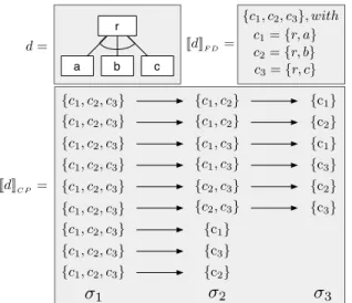
![Figure 1. FD example, adapted from [8].](https://thumb-eu.123doks.com/thumbv2/123doknet/14573946.728157/4.918.154.354.105.240/figure-fd-example-adapted-from.webp)
![Figure 2. Specialisation steps, adapted from [8].](https://thumb-eu.123doks.com/thumbv2/123doknet/14573946.728157/6.918.86.818.109.211/figure-specialisation-steps-adapted-from.webp)
![Table 2. Possible inter-level links; original definition [8] left, translation to FD semantics right.](https://thumb-eu.123doks.com/thumbv2/123doknet/14573946.728157/7.918.85.812.133.562/table-possible-inter-level-original-definition-translation-semantics.webp)
+3
![Figure 6. Example of Figure 3 in [[d]] CP and [[d]] DynF D .](https://thumb-eu.123doks.com/thumbv2/123doknet/14573946.728157/10.918.118.782.107.559/figure-example-figure-d-cp-d-dynf-d.webp)
Documents relatifs