HAL Id: inria-00156747
https://hal.inria.fr/inria-00156747v5
Submitted on 28 Jun 2007
HAL is a multi-disciplinary open access
archive for the deposit and dissemination of sci-entific research documents, whether they are pub-lished or not. The documents may come from teaching and research institutions in France or abroad, or from public or private research centers.
L’archive ouverte pluridisciplinaire HAL, est destinée au dépôt et à la diffusion de documents scientifiques de niveau recherche, publiés ou non, émanant des établissements d’enseignement et de recherche français ou étrangers, des laboratoires publics ou privés.
Optimal Replica Placement in Tree Networks with QoS
and Bandwidth Constraints and the Closest Allocation
Policy
Veronika Rehn-Sonigo
To cite this version:
Veronika Rehn-Sonigo. Optimal Replica Placement in Tree Networks with QoS and Bandwidth Constraints and the Closest Allocation Policy. [Research Report] RR-6233, INRIA. 2007. �inria-00156747v5�
inria-00156747, version 5 - 28 Jun 2007
a p p o r t
d e r e c h e r c h e
IS S N 0 2 4 9 -6 3 9 9 IS R N IN R IA /R R --6 2 3 3 --F R + E N G Thème NUMINSTITUT NATIONAL DE RECHERCHE EN INFORMATIQUE ET EN AUTOMATIQUE
Optimal Replica Placement in Tree Networks with
QoS and Bandwidth Constraints and the Closest
Allocation Policy
Veronika Rehn-Sonigo
N° 6233
Unité de recherche INRIA Rhône-Alpes
655, avenue de l’Europe, 38334 Montbonnot Saint Ismier (France)
Téléphone : +33 4 76 61 52 00 — Télécopie +33 4 76 61 52 52
Optimal Replica Placement in Tree Networks with QoS and
Bandwidth Constraints and the Closest Allocation Policy
Veronika Rehn-Sonigo
Th`eme NUM — Syst`emes num´eriques Projet GRAAL
Rapport de recherche n°6233 — June 2007 —13 pages
Abstract: This paper deals with the replica placement problem on fully homogeneous tree networks known as the Replica Placement optimization problem. The client requests are known beforehand, while the number and location of the servers are to be determined. We investigate the latter problem using the Closest access policy when adding QoS and bandwidth constraints. We propose an optimal algorithm in two passes using dynamic programming. Key-words: Replica placement, tree networks, Closest policy, quality of service, bandwidth constraints.
This text is also available as a research report of the Laboratoire de l’Informatique du Parall´elisme http://www.ens-lyon.fr/LIP.
Placement optimal de r´
epliques dans les r´
eseaux en arbre avec
des contraintes de qualit´
e de service et de bande passante et
avec la politique d’allocation Closest
R´esum´e : Dans ce papier, nous traitons le probl`eme du placement de r´epliques dans des r´eseaux en arbres compl`etement homog`enes, connu sous le nom du probl`eme d’optimisation de Replica Placement. Les requˆetes des clients sont connues a priori, mais le nombre et les emplacements des serveurs restent `a d´eterminer. Nous ´etudions ce dernier probl`eme en utilisant la politique d’acc`es Closest, en ajoutant de la qualit´e de service et des limitations de bande passante. Nous proposons un algorithme optimal en deux passes qui utilise la programmation dynamique.
Mots-cl´es : Placement de r´epliques, r´eseaux en arbres, politique Closest, qualit´e de service, limitation de bande passante.
Optimal Replica Placement in Tree Networks 3
1
Introduction
This paper deals with the problem of replica placement in tree networks with Quality of Service (QoS) guarantees and bandwidth constraints. Informally, there are clients issuing several requests per time-unit, to be satisfied by servers with a given QoS and respecting the bandwidth limits of the interconnection links. The clients are known (both their position in the tree and their number of requests), while the number and location of the servers are to be determined. A client is a leaf node of the tree, and its requests can be served by one or several internal nodes. Initially, there are no replicas; when a node is equipped with a replica, it can process a number of requests, up to its capacity limit (number of requests served by time-unit). Nodes equipped with a replica, also called servers, can only serve clients located in their subtree (so that the root, if equipped with a replica, can serve any client); this restriction is usually adopted to enforce the hierarchical nature of the target application platforms, where a node has knowledge only of its parent and children in the tree. Every client has some QoS constraints: its requests must be served within a limited time, and thus the servers handling these requests must not be too far from the client.
The rule of the game is to assign replicas to internal nodes so that some optimization function is minimized and QoS as well as bandwidth constraints are respected. Typically, this optimization function is the total utilization cost of the servers. We restrict the problem to the most popular access policy called Closest, where each client is allowed to be served only by the closest replica in the path from itself up to the root.
In this paper we study this optimization problem, called Replica Placement, and we restrict the QoS in terms of number of hops. This means for instance that the requests of a client who has a QoS range of 5 must be treated by one of the first five internal nodes on the path from the client up to the tree root.
We point out that the distribution tree (clients and nodes) is fixed in our approach. This key assumption is quite natural for a broad spectrum of applications, such as electronic, ISP, or VOD service delivery. The root server has the original copy of the database but cannot serve all clients directly, so a distribution tree is deployed to provide a hierarchical and distributed access to replicas of the original data. On the contrary, in other, more decentralized, applications (e.g. allocating Web mirrors in distributed networks), a two-step approach is used: first determine a “good” distribution tree in an arbitrary interconnection graph, and then determine a “good” placement of replicas among the tree nodes. Both steps are interdependent, and the problem is much more complex, due to the combinatorial solution space (the number of candidate distribution trees may well be exponential).
Many authors deal with the Replica Placement optimization problem. Most of the papers neither deal with QoS nor with bandwidth constraints. Instead they consider average system performance as total communication cost or total accessing cost. Please refer to [2] for a detailed description of related work with no QoS constraints.
Cidon et al. [3] studied an instance of Replica Placement with multiple objects, where all requests of a client are served by the closest replica (Closest policy). In this work, the objective function integrates a communication cost, which can be seen as a substitute for QoS. Thus, they minimize the average communication cost for all the clients rather than ensuring a given QoS for each client. They target fully homogeneous platforms since there are no server capacity constraints in their approach. A similar instance of the problem has been studied by Liu et al [6], adding a QoS in terms of a range limit, and whose objective is to minimize the
4 V. Rehn-Sonigo
number of replicas. In this latter approach, the servers are homogeneous, and their capacity is bounded. Both [3,6] use a dynamic programming algorithm to find the optimal solution.
Some of the first authors to introduce actual QoS constraints in the problem were Tang and Xu [7]. In their approach, the QoS corresponds to the latency requirements of each client. Different access policies are considered. First, a replica-aware policy in a general graph with heterogeneous nodes is proven to be NP-complete. When the clients do not know where the replicas are (replica-blind policy), the graph is simplified to a tree (fixed routing scheme) with the Closest policy, and in this case again it is possible to find an optimal dynamic programming algorithm.
Bandwidth limitations are taken into account when Karlsson et al. [5,4] compare different objective functions and several heuristics to solve NP-complete problem instances. They do not take QoS constraints into account, but instead integrate a communication cost in the objective function as was done in [3]. Integrating the communication cost into the objective function can be viewed as a Lagrangian relaxation of QoS constraints. Please refer to [1] for more related work dealing with QoS constraints.
In this paper we propose an efficient algorithm called Optimal Replica Placement (ORP ) to determine optimal locations for placing replicas in the Replica Placement prob-lem including QoS and bandwidth. Our work provides a major extension of the algorithm of Liu et al. [6], which was already mentioned above. Liu et al. [6] proposed an algorithm Place-replica to find an optimal set of replicas on homogeneous data grid trees including QoS constraints in terms of distance but without bandwidth constraints. Our approach leads to two important extensions. First of all, we separate the set of clients from the set of servers, while Liu et al suppose clients to be servers with a double functionality. Our model can simulate the latter model while the converse is not true. Indeed, we can model client-server nodes by inserting a fictive node before the client which can take the role of a server. The approach of Liu et al. in contrast does not offer the possibility to model clients without server functionality.
Our second major contribution is the introduction of bandwidth constraints. This is an important modification of the requirements as QoS and bandwidth are of a completely different nature. QoS is a constraint that belongs to a node locally, hence each client has to cope with its own limitation. Bandwidth constraints in contrast have a global influence on the resources as a link may be shared by multiple clients and consequently all of them are concerned. Therefore it is not obvious whether the problem with these completely different constraint types would remain polynomial or would become NP-hard.
The rest of the paper is organized as follows. Section 2 introduces our main notations used in Replica Placement problems. Section 3 is dedicated to the presentation of our polynomial algorithm: the proper terminology of the algorithm is introduced in Section3.0.1. The subsections3.1and 3.3treat the different phases and explaining examples can be found in Sections3.2and3.4. Complexity is subject of Section3.5, whereas optimality is proven in Section3.6. Section 4summarizes our work.
2
Notations
This section familiarizes with our basic notations. We consider a distribution tree T whose nodes are partitioned into a set of clients C and a set of internal nodes N (N ∩ C = ∅). The clients are leaf nodes of the tree, while N is the set of internal nodes. Let r be the root of
Optimal Replica Placement in Tree Networks 5 r r+ 0
T
Figure 1: Appearance of T∗the tree. The set of tree edges (links) is denoted as L. Each link l owns a bandwidth limit BW(l) that can not be exceeded.
A client v ∈ C is making wv requests per time unit to a database. Each client has to respect its personal Quality of Service constraints (QoS), where q(v) indicates the range limit in hops for v upwards to the root until a database replica has to be reached. A node j ∈ N may or may not have been provided with a replica of the database. Nodes equipped with a replica (i.e. servers) can process up to W requests per time unit from clients in their subtree. In other words, there is a unique path from a client v to the root of the tree, and each node in this path is eligible to process all the requests issued by v when provided with a replica. We denote by R ⊆ N the entire set of nodes equipped with a replica.
3
Optimal Replica Placement Algorithm (ORP)
In this section we present ORP , an algorithm to solve the Replica Placement problem using the Closest policy with QoS and bandwidth constraints. For this purpose, we modify an algorithm of Lin, Liu and Wu [6]. Their algorithm Place-replica is used on homogeneous conditions with QoS constraints but without bandwidth restrictions. To be able to use the algorithm, we have to modify the original platform. We transform the tree T in a tree T∗ by adding a new root r+ as father of the original root r (see Figure 1). r+ is connected to r via a link l0, where BW(l0) = 0. As the bandwidth is limited to 0, no requests can pass above r, so that this artificial transformation for computation purposes can be adapted to any tree-network.
A further, only formal transformation, consists in the suppression of clients from the tree and hence the consideration of their parents as leaves in the following way (Figures 2
and3 give an illustration): for every parent v who has only leaf-children v1, .., vn (i.e., all its children are clients), we assign the sum of the requests of the vj as its requests w(v), i.e., w(v) =P
1≤j≤nw(vj). The associated QoS is set to (min1≤j≤nq(vj))−1. This transformation is possible, as we use the Closest policy and hence all children have to be treated by the same server. From those parents who have some leaf-children v1, .., vn, but also non-leaf children vn+1, .., vm, the clients can not be suppressed completely. In this case the leaf-children v1, .., vn are compressed to one single client c with requests w(c) = P1≤j≤nw(vj) and QoS q(c) = min1≤j≤nq(vj). Once again this compression is possible due to the restriction on the Closest access policy.
6 V. Rehn-Sonigo v1 vj v w(v1) w(vj) w(vn) q(v1) q(vj) q(vn) vn
(a) Node v before suppression of clients.
v w(v) =P
1≤j≤nw(vj)
(min1≤j≤nq(vj)) − 1
(b) Node v after suppression of clients.
Figure 2: Suppression of clients
v
v1 vn
w(vn)
w(v1)
q(v1) q(vn)
(a) Node v before compression of its clients. v c w(c) =P 1≤j≤nw(vj) q(c) = min1≤j≤nq(vj)
(b) Node v after compression of its clients.
Figure 3: Compression of clients.
ORP works in two phases. In the first phase so called Contribution Functions are com-puted which will serve in the second phase to determine the optimal replica placements. In the following some new terms are introduced and then the two phases are described in detail. 3.0.1 Terminology
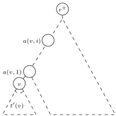
Working with a tree T∗ with root r+, we note t(v) the subtree rooted by node v, and t′(v) = t(v) − v, i.e. the forest of trees rooted at v’s children. The i’th ancestor of node v, traversing the tree up to the root, is denoted by a(v, i).
Using these notations, we denote m(T∗) the minimum cardinality set of replicas that has to be placed in tree T such that all requests can be treated by a maximum processing capacity of W (respecting QoS and bandwidth constraints). In the same manner m(t(v)) denotes the minimum number of replicas that has to be placed in t′(v), such that the remaining requests on node v are within W . For this purpose we define a contribution function C. C(v, i) denotes the minimum workload on node a(v, i) contributed by t(v) by placing m(t(v)) replicas in t′(v) and none on a(v, j) for 0 ≤ j < i. The computation and an illustrating example are presented below (Cf. Section 3.2and Section 3.4). But before we need a last notation. The set e(v, i) denotes the children of node v that have to be equipped with a replica such that the remaining requests on node a(v, i) are within W , there are exactly m(t(v)) replicas in t′(v) and none
Optimal Replica Placement in Tree Networks 7 v t′(v) r+ a(v, 1) a(v, i)
Figure 4: Clarification of the terminology.
on a(v, j) for 0 ≤ j < i and the contribution t(v) on a(v, i) is minimized. The computation formula is also given below. Of course the compression of leaves is not possible if a client v of the original tree T is connected to its father via a communication link l that has a lower bandwidth than v requests (BW(l) < w(v)). In this case we know a priori that there is no solution to our problem as v’s requests can not be treated.
3.1 Phase 1: Bottom up computation of set e, amount m and contribution
function C
The computation of e, m and C is a bottom up process, distinguishing two cases. 1. v is a leaf:
In this case we do not need e and m and we can directly compute the contribution function. C(v, i) is w(v) when (i ≤ q(v) ∧ w(v) ≤ minBWpath[v → a(v, i)]), and infinity otherwise.
We point out that there is no solution if any of the leaves has more requests than W or if the bandwidth of any of the clients to its parent is not sufficiently high.
2. v is an internal node with children v1, . . . , vn:
i= 0: If the contribution on v of its children, i.e. the incoming requests on v is bigger than the processing capacity of inner nodes W , we know we have to place some replicas on the children to bound the incoming requests on W . To find out which children have to be equipped with a replica, we take a look at the C(vj,1)-values of the children. The set e(v, 0) is used to store the vj’s that are determined to be equipped with a replica. Hence the procedure is the following:
e(v, 0) = ∅ while(
P
vj∈e(v,0)/ C(vj,1) > W )
add vj ∈ N with biggest C(vj,1) to e(v, 0)
Note that the set N used in the procedure still corresponds to the set of internal nodes of the original tree T . So we can add leaf nodes of T∗ that are inner nodes in T , but we can not add compressed client nodes. Note furthermore that there is no client that is added to e(v, 0). Besides we remark that there is no valid solution within W and the present QoS and bandwidth constraints, when all children vj ∈ N
8 V. Rehn-Sonigo
of v are equipped with a replica and the incoming requests do not fit in W . Of course this holds also true in the case i > 0. Subsequently, the value of m(t(v)) is determined easily: m(t(v)) =P
1≤j≤nm(t(vj)) + |e(v, 0)|. We remind that m(t(v)) indicates the minimum number of replicas that have to be placed in t′(v) to keep the number of contributed requests inferior to W . Finally, the computation of the contribution function :
C(v, 0) = X vj∈e(v,0)/
C(vj,1) .
i >0: Treating node v, we want to compute the contribution on a(v, i). As for i = 0, we start computing the set e(v, i):
e(v, i) = ∅ while(
P
vj∈e(v,i)/ C(vj, i+ 1) > W )
add vj ∈ N with biggest C(vj, i+ 1) to e(v, i)
The computation of the contribution function follows a similar principle: C(v, i) =
(P
vj∈e(v,i)/ C(vj, i+ 1), if |e(v, i)| = |e(v, 0)|
∞, otherwise (1)
C(v, i) is set to ∞, when the number of |e(v, 0)| replicas placed among the children of v is not sufficient to keep the contributed requests on a(v, i) within W .
3.2 Example of Phase 1
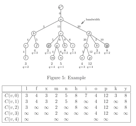
Consider the tree in Figure 5and a processing capacity of inner nodes fixed to W = 15. The tree has already been transformed. So nodes x and y are compressed client-leaves (grey scaled in the figure), whereas all other leaves correspond to servers (former inner nodes, hence nodes that are within N ). We start with the computation of all C(v, i)-values of all leaves. Leaf l for example has C(l, 0) = 3 as it holds 3 requests. As the link from l to e has a bandwidth of 4, and the QoS is 2, the requests of l can ascent to node e and hence the contribution of l’s requests on node e, C(l, 1), is 3. In the same manner, C(l, 2), i.e. the contribution of l’s requests on node b is 3 as well. But then the QoS range is exceeded and hence the requests of l can not be treated higher in the tree. Consequently the contributions on nodes a and a+ (C(l, 3) and C(l, 4)) are set to infinity. Another example: Leaf i owns 7 requests, but the link from i to its parent c has a lower bandwidth, and hence the contribution of i on c, C(i, 1), has to be set to infinity. The whole computation table for the leaf-contributions is given in Table 1.
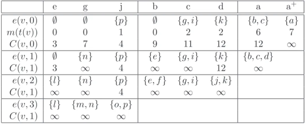
Table 2 is used for the computation of e, m and C values of inner nodes. During the computation process it is filled by main columns, where one main column consists of all inner nodes of the same level in the tree. So we start with node e. The contribution of its child l, C(l, 1), is 3 as we computed in Table 1. And as it is the only child, we have that the contributed requests on e are less than the processing capacity W which is fixed to 15 and hence we do not need to place a replica on the child l of e to minimize the contribution on e. Corresponding we get m(t(e)) = 0, i.e. we do not need to place a replica in the subtree t′(e), and a contribution C(e, 0) = 3. e(e, 1) and C(e, 1) are computed in the same manner, taking into account C(l, 2). Computing e(e, 2), i.e. the nodes that have to be equipped with
Optimal Replica Placement in Tree Networks 9 i h m n g a+ a c x y b e f l bandwidth d j k p o 7 8 6 4 2 5 0 15 6 9 6 5 10 4 4 5 4 3 8 3 20 3 12 20 2 3 4 12 5 q = 3 q = 2 q = 1 q = 4 q = 3 q = 2 q = 1 q = 3 q = 2 q = 4 q = 3 Figure 5: Example l f x m n h i o p k y C(v, 0) 3 4 3 2 5 8 7 4 12 3 8 C(v, 1) 3 4 3 2 5 8 ∞ 4 12 ∞ 8 C(v, 2) 3 ∞ ∞ 2 ∞ 8 ∞ 4 12 ∞ 8 C(v, 3) ∞ ∞ ∞ 2 ∞ ∞ ∞ 4 12 ∞ ∞ C(v, 4) ∞ ∞ ∞ ∞ ∞
Table 1: Computation of C(v, i)-values of leaves.
a replica if we want to minimize the contribution on node a(e, 2) = a by placing replicas on the children of e but none on e up to a. For this purpose we use C(l, 3), the contribution of l on a and remark that it is infinity. Hence we have ∞ > W = 15 and so we have to equip l with a replica, and as now the set e(e, 2) has a higher cardinality than e(e, 0), we know that this solution is not optimal anymore and we set the contribution of C(e, 2) to infinity (Eq.1). Taking a look at node j: In the computation of e(j, 0), we have a total contribution of its children of 16, which exceeds the processing power of W = 15 (bandwidth and QoS are not restricting here). So we know that we have to equip one of the children with a replica, and we choose the one with the highest contribution on j: node p. Consequently, we get m(t(j)) = 1 as we have to place one replica on the children. The contribution C(j, 0) consists in the 4 remaining contributed requests of node o. Once we have finished all computations for this level, we start with the computations of the next level, which can be found in the next main column of the table. Let us treat exemplarily node c. The sum of its children’s contributions is C(x, 1) + C(g, 1) + C(h, 1) + C(i, 1) = ∞ as C(g, 1) = C(i, 1) = ∞. So we add g and i to e(c, 0) to lower the contributions to C(x, 1) + C(h, 1) = 11 which fits in the processing power of W = 15. The outcome of this is m(t(c)) = 2 and the remaining requests lead to C(c, 0) = 11.
3.3 Phase 2: Top down replica placement
The second phase uses the precomputed results of the first phase to decide about the nodes on which to place a replica. The goal is to place m(T∗) = m(t(r+)) replicas in t′(r+). Note that this means that there is no replica on r+ and hence only the original tree T will be equipped with replicas. If the workload on node r is within W , we have a feasible solution.
10 V. Rehn-Sonigo e g j b c d a a+ e(v, 0) ∅ ∅ {p} ∅ {g, i} {k} {b, c} {a} m(t(v)) 0 0 1 0 2 2 6 7 C(v, 0) 3 7 4 9 11 12 12 ∞ e(v, 1) ∅ {n} {p} {e} {g, i} {k} {b, c, d} C(v, 1) 3 ∞ 4 ∞ ∞ 12 ∞ e(v, 2) {l} {n} {p} {e, f } {g, i} {j, k} C(v, 1) ∞ ∞ 4 ∞ ∞ ∞ e(v, 3) {l} {m, n} {o, p} C(v, 1) ∞ ∞ ∞
Table 2: Computation of e, m and C for internal nodes.
Phase 2 is a recursive approach. Starting with i = 0 on node v = r+, all nodes that are within e(v, i) are equipped with a replica. In this top down approach, i indicates the distance of node v to its first ancestor up in the tree that is equipped with a replica and hence the set e(v, i) denotes the set of children of v that have to be equipped with a replica in order to minimize the contribution of v on a(v, i). Next the procedure is called recursively with the appropriate index i. Algorithm1 gives the pseudo-code for the top down placement phase, which is the same as the one in [6].
procedure Place-replica (v, i) begin
if v∈ C then return; end
place a replica at each node of e(v, i); forallc∈ children(v) do if c∈ e(v, i) then Place-replica(c,0); else Place-replica(c,i+1); end end end
Algorithm 1: Top down replica placement
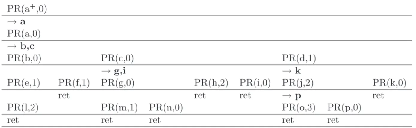
3.4 Example of Phase 2
We start with the results of Phase 1 (Cf. Table 1 and 2) and call then the procedure Place-replica (Algorithm 1) with (a+,0). a+ is not a leaf, so we place a replica on its child a, as a∈ e(a, 0) and then recall the procedure with (a, 0). This time we place replicas on b and c and call the procedure with values (b, 0), (c, 0) and (d, 1). We have to increment i to 1 when we treat node d, as we already know that we will not equip d with a replica, and hence the children of d might give their contribution directly to a. So we have to examine which of the children of d have to be equipped with a replica, to minimize the contribution on a. This is stored in the e(vj,1)-values of all children vj of d. So every time we do not place a replica
Optimal Replica Placement in Tree Networks 11 PR(a+,0) → a PR(a,0) → b,c PR(b,0) PR(c,0) PR(d,1) → g,i → k PR(e,1) PR(f,1) PR(g,0) PR(h,2) PR(i,0) PR(j,2) PR(k,0)
ret ret ret → p ret
PR(l,2) PR(m,1) PR(n,0) PR(o,3) PR(p,0)
ret ret ret ret ret
Table 3: Scheme on the recursive calls of the procedure Place-replica
on a node and descent to its children, we increase the distance-indicator i to the first replica that can be found the way up to the root. The recursive procedure call for the entire example is given in Table 3.4. PR(x,i) stands for the call of Place-replica with parameters (x,i) and → x indicates that node x is equipped with a replica.
3.5 Complexity
Let us take a look on the complexity of ORP . For each node v we have to compute e, m and C values. So the computation requires n log n, if v has n children and if we sort the C values from all of v’s children. We have to do at most L sorting, where L is the maximum range limit among all nodes. So at all the computation complexity for the values for one node is Lnlog n, and we get a total complexity of LN log N , where N is the number of nodes in the tree.
3.6 Optimality
In this section we prove optimality of our algorithm ORP by recursion over levels. For this purpose we apply a theorem introduced by Liu et al. [6] and presented below as Theorem1. Liu et al. used this theorem in order to prove the existence of an optimal solution on a homogeneous data grid tree under QoS constraints. As the theorem does not take into account if there are any constraints like QoS or bandwidth, we can adopt it for our problem.
Theorem 1. Consider a data grid tree T , a node v in T with children v1, .., vnand a workload W. There exists a replica set R so that |R| = m(T ), R minimizes the total workload due to R from t′(v) on a(v, i) for i ≥ 1, and |R ∩ t′(v
j)| = m(t(vj)).
In other words, Theorem1 guarantees that for a tree T with fixed processing capacity W there exists a replica set R whose cardinality is the minimum number of replicas that has to be placed in t′(r) (where r is the root of T ), such that the remaining requests on r are within W. Furthermore for a node v with children v1, ..., vn, due to R the workload on a ancestor a(v, i) of v is minimized and the number of replicas that are placed in the subtree t′(vj) is minimal.
Proof. We can use the same arguments as Liu et al. as we did not change the definition of m-values but the constraints on m. By definition of m(t(vj)), we know that this is the
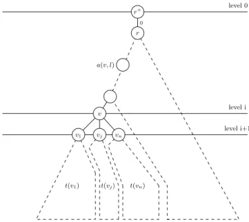
12 V. Rehn-Sonigo level 0 level i level i+1 0 r+ r v v1 vj vn t(v1) t(vj) t(vn) a(v, l)
Figure 6: Induction over levels. minimal number of replicas that has to be placed in t′(v
j) such that the contribution on vj is within W . Hence |R ∩ t′(vj)| can not be less than m(t(vj)) because otherwise the contribution on vj would exceed W . On the other side in any optimal solution for t(vj), we can not place more replicas in t′(v
j) than m(t(vj)) and than one more on vj. The resulting contribution on a(v, i) decreases at most when placing the replica on vj.
Theorem 2. Algorithm ORP returns an optimal solution to the Replica Placement prob-lem with fixed W , QoS and bandwidth constraints, if there exists a solution.
Proof. We perform an induction over levels to prove optimality. We consider any tree T∗ of hight n + 1 and start at level 0, which consists in the artificial root r+ (Cf. Figure 6). level 0: Using Theorem 1, we know that there exists an optimal solution R0 for our tree
(i.e., a set R of replicas whose cardinality is m(T∗)) such that |R0 ∩ t′(r)| = m(t(r)). We have m(T∗) = m(t(r)) + |e(r+,0)| by definition of e(r+,0). Hence e(r+,0) = {r} if and only if r ∈ R0. This is exactly how the algorithm pursuits.
level i → i+1: We assume that we have placed the replicas from level 0 to level i (with Algorithm1) and that there exists an optimal solution Riwith these replicas. We further suppose that for each node v in level i it holds |Ri∩ t′(v)| = m(t(v)). Let us consider a node v in level i with children v1, .., vn and we define l := min{k ≥ 0|a(v, k) ∈ Ri}. In the next step of the algorithm we equip the elements of e(v, l) with a replica. We have m(t(v)) =P
1≤j≤nm(t(vj)) + |e(v, 0)|, i.e. the minimal number of replicas in the subtrees t′(vj) and the minimal number of replicas on the children of v that have to be placed to keep the contributed requests on v within W . By definition of e(v, l) we have that |{j ∈ {1, .., n}|vj ∈ Ri}| ≥ |e(v, l)| and we also have |e(v, l)| = |e(v, 0)| as the contribution C(v, l) is finite and Ri a solution. For the inequality, there is even equality because otherwise there would exist a j such that |t′(v
j) ∩ Ri| < m(t(vj)), which is impossible. With this equality, we can replace the children of v that are in Ri by the
Optimal Replica Placement in Tree Networks 13
children of v that are in e(v, l) creating a solution Ri+1. So Ri+1 is also an optimal solution, because |Ri| = |Ri+1| (we did not change the nodes of the other levels) and the contribution of t(v) on a(v, l) has at most decreased. Furthermore for every node v′ at level i+1 we have |Ri+1∩ t′(v′)| = m(t(v′)).
So the last solution Rn that we get in the induction step n is optimal and it corresponds to the solution that we obtain by our algorithm.
4
Conclusion
In this paper we dealt with the Replica Placement optimization problem with QoS and bandwidth constraints. We restricted our research on Closest/Homogeneous instances. We were able to prove polynomiality and proposed the optimal algorithm ORP . This algorithm extends an existing algorithm in two important areas. First the set of clients and the set of servers can be distinct now and does not require exclusively double-functionality nodes anymore. The other major contribution is the expansion to the interplay of different nature constraints. QoS, which is a proper constraint for each client, and bandwidth, a global resource limitation, subordinate to a common optimization function. This accomplishment completes furthermore the study on complexity of Closest/Homogeneous in tree networks.
References
[1] A. Benoit, V. Rehn, and Y. Robert. Impact of QoS on Replica Placement in Tree Networks. Research Report 2006-48, LIP, ENS Lyon, France, Dec. 2006. Available at graal.ens-lyon.fr/~yrobert/.
[2] A. Benoit, V. Rehn, and Y. Robert. Strategies for Replica Placement in Tree Net-works. Research Report 2006-30, LIP, ENS Lyon, France, Oct. 2006. Available at graal.ens-lyon.fr/~yrobert/.
[3] I. Cidon, S. Kutten, and R. Soffer. Optimal allocation of electronic content. Computer Networks, 40:205–218, 2002.
[4] M. Karlsson and C. Karamanolis. Choosing Replica Placement Heuristics for Wide-Area Systems. In ICDCS ’04: Proceedings of the 24th International Conference on Distributed Computing Systems (ICDCS’04), pages 350–359, Washington, DC, USA, 2004. IEEE Computer Society.
[5] M. Karlsson, C. Karamanolis, and M. Mahalingam. A framework for evaluating replica placement algorithms. Research Report HPL-2002-219, HP Laboratories, Palo Alto, CA, 2002.
[6] P. Liu, Y.-F. Lin, and J.-J. Wu. Optimal placement of replicas in data grid environments with locality assurance. In International Conference on Parallel and Distributed Systems (ICPADS). IEEE Computer Society Press, 2006.
[7] X. Tang and J. Xu. QoS-Aware Replica Placement for Content Distribution. IEEE Trans. Parallel Distributed Systems, 16(10):921–932, 2005.
Unité de recherche INRIA Rhône-Alpes
655, avenue de l’Europe - 38334 Montbonnot Saint-Ismier (France)
Unité de recherche INRIA Futurs : Parc Club Orsay Université - ZAC des Vignes 4, rue Jacques Monod - 91893 ORSAY Cedex (France)
Unité de recherche INRIA Lorraine : LORIA, Technopôle de Nancy-Brabois - Campus scientifique 615, rue du Jardin Botanique - BP 101 - 54602 Villers-lès-Nancy Cedex (France)
Unité de recherche INRIA Rennes : IRISA, Campus universitaire de Beaulieu - 35042 Rennes Cedex (France) Unité de recherche INRIA Rocquencourt : Domaine de Voluceau - Rocquencourt - BP 105 - 78153 Le Chesnay Cedex (France)
Unité de recherche INRIA Sophia Antipolis : 2004, route des Lucioles - BP 93 - 06902 Sophia Antipolis Cedex (France)
Éditeur
INRIA - Domaine de Voluceau - Rocquencourt, BP 105 - 78153 Le Chesnay Cedex (France)
http://www.inria.fr