HAL Id: hal-02080069
https://hal-amu.archives-ouvertes.fr/hal-02080069
Submitted on 26 Mar 2019HAL is a multi-disciplinary open access archive for the deposit and dissemination of sci-entific research documents, whether they are pub-lished or not. The documents may come from teaching and research institutions in France or abroad, or from public or private research centers.
L’archive ouverte pluridisciplinaire HAL, est destinée au dépôt et à la diffusion de documents scientifiques de niveau recherche, publiés ou non, émanant des établissements d’enseignement et de recherche français ou étrangers, des laboratoires publics ou privés.
Distributed under a Creative Commons Attribution| 4.0 International License
Discrete-Time Systems Via Three Terms approximation
El Mostafa El Adel, H Aiss, A. Hmamed
To cite this version:
El Mostafa El Adel, H Aiss, A. Hmamed. Delay Dependent Stability Criteria and Stabilization for Discrete-Time Systems Via Three Terms approximation. Journal of Control Engineering and Applied Informatics, SRAIT, 2017, 19, pp.3 - 12. �hal-02080069�
CEAI, Vol.19, No.4 pp. 3-12, 2017 Printed in Romania
Delay Dependent Stability Criteria and Stabilization for Discrete-Time
Systems Via Three Terms approximation
H. El Aiss*, A. Hmamed, M. EL Adel**
* Department of Physics, Faculty of Sciences Dhar El Mehraz, University of Sidi Mohamed Ben Abdellah, B.P. 1796 Fes-Atlas Morocco.
(e-mail: [email protected], hammed [email protected]). ** LSIS-UMR 6168, University of Paul Cezane, Aix-Marseille, France.
(e-mail: [email protected])
Abstract: This paper discusses the problem of delay-dependent stability and stabilization condition for
discrete-time linear systems. By employing a three-term approximation for delayed state variables, a new model transformation is developed, which has a smaller approximation error than the two-term approach. By using scaled small gain theorem and an appropriate Lyapunov-Krasovskii functional, new delay-dependent stability conditions are proposed and formulated as linear matrix inequalities (LMIs). Before the end, a state feedback controller has investigated in the stabilization of discrete linear systems. Finally, numerical examples are presented to illustrate the effectiveness of the proposed method.
Keywords: Discrete time delay; Linear Matrix Inequality (LMI); Scaled Small Gain Theorem;
Time-Delay system.
1. INTRODUCTION
Time delays are often an integral part of various physical systems like air-craft stabilization, communication systems, population dynamics, ship stabilization, electric power systems with lossless transmission lines and nuclear reactors, etc. The nature of these delays is time-varying. It is well known that the existence of time delay in various systems may provide poor performance and instability of dynamic systems, for more details see (Kim, 2011; Lakshmanan et al., 2011; Sun et al., 2010; Xu and Lam, 2008) and references therein.
Recently, the discrete time modelling has an essential role in many fields of science and engineering. Thus, most of systems are implemented with digital computers via the necessary input/output hardware. The digital computer uses the information in a way discrete. For the aforementioned considerations, much interest has been fixed to the analysis of discrete-time delay systems see for example (Chen et al., 2003; He et al., 2007; Lin et al., 2006; Park, 1999; Xu and Lam, 2005). Based on Lyapunov-krasovskii functional and on bounding techniques, delay-dependent stability of discrete-time systems has been investigated by (Fridman and Shaked, 2005; Gao and Chen, 2007; Gao et al., 2004; Jiang et al., 2005). On the other hand, many authors have been employed the input/output approach in the stability analysis of time-delay systems. This method is based on a specific transformation which aims to transform a pure system into two interconnected subsystems.
The input/output approach has been implemented in various works. Many works have proposed some results such as (Huang and Zhou, 2000; Park, 1999) for constant delays, and
it has been extended to time varying delay in (Fridman and Shaked, 2007; Kao and Rantzer, 2007). For time varying delay, the idea is to find an approximation of x k d k( ( )) for discrete-time case or x t h t( ( )) for continuous-time case, such that its approximation error is small as possible. (Fridman and Shaked, 2007) have adopted x k( da
)
as the approximation of x k( d k( )) with da = (d1 + d2)/2, and1
(
)
x kd is used by (Kao and Lincoln, 2004). (Gu et al., 2011; Hmamed et al., 2015) have introduced the two term approximation
x t h( 1)
x t h( 2) 2
as the approximation of x t h(
t
)
for continuous-time delayed case, and (Zhao et al., 2013) for T-S Fuzzy systems with time-varying delay. (Li and Gao, 2011) have also used the discrete two term approximation
x t d( 1)
x t d( 2) 2
as the approximation of x k( d k( ))for discrete delay systems. The same approximation has been considered in (Su et al., 2012) for filtering T-S fuzzy discrete-time systems with time-varying delay. It is pointed out that the approximation model of the delayed state with two terms is better than that based on only one term.In this paper, Three terms approximation is proposed by using
x k( d1)
x k( d2)
x k( da) 3
as an approximation of x k( d k( )) with d1 and d2 being the lower and the upper bounds of delay, within which the approximation error is smaller than the two-terms (Li and Gao, 2011). Then a new model transformation is formulated and will be analyzed and applied for the stability analysis andstabilization of discrete delay systems. By using an appropriate Lyapunov-Krasovskii functional and the scaled small gain theorem (SSG) we present a new stability criterion of a subsystem. Before the end, the conditions which guarantee that discrete system is asymptotically stable under state feedback controller are given as LMIs by using the cone complementarity linearization algorithms. Finally, Numerical examples are given to illustrate the effective of the proposed method.
Notations: Notation P > 0(≥0) means that matrix P Is
positive (semi) definite. The Superscript 'T' means the transpose. G1●G2 denotes the series connection of G1 and G2.
I is an identity matrix with appropriate dimension. Denote
“*” for the terms that can be deduced by symmetry In block matrices, we use diag{...} to express a block- diagonal matrix. 2 2 0 ( ) ( ) T l k x x k x k
denotes the l2 norm of series
x(k) and ‖ꞏ‖∞ represents the l2-induced norm of a transfer
function matrix or a general operator.
2. PROBLEM FORMULATION AND PRELIMINARIES We consider the discrete time linear system with an interval time delay described by the following model.
2 2 ( 1) ( ) ( ( )) ( ) ( ), , 1,...,0 d x k Ax k A x k d k x k
k k d d (1)Where
x k
( )
n is the state vector,,
n n dA A
are constant matrices,
( ),
k
k
d
2,
d
21,...,0
is the given initial condition sequence.( )
d k
is the time delay, time-varying satisfying.1 2
1
d
d k
( )
d
(2) where d1 and d2 are known constants.Before proceeding on, the following lemma is introduced which plays an important part in the development of our main results.
Lemma 1. (Huang and Feng, 2010) For any symmetric
matrix M 0, integer l1l2and vector function
1 1 2
: ,l l 1,...,l n
such that the sums concerned are well defined, then2 2 2 1 1 1 2 1 ( 1) ( ) ( ) ( ) ( ) T l l l T i l i l i l l l i M i i M i
The main objective of this work is to determine the stability condition for time delay system (1) using the Scaled Small Gain Theorem (SSG) (Li and Gao, 2011). To apply this theorem, we need to transform the original system (1) into the two following subsystems:
1 2
( ) : ( )S z t G t( ); ( ) : ( )S t z t( ) (3) Where the forward S1 is a known linear time-invariant (LTI)
system with operator G mapping
( )
t
to z(t), and the feedback S2 is an unknown linear time-varying one withoperator
D
:
1
,z t
( )
z and( )
t
. From the SSG Theorem in (Li and Gao, 2011), we derive sufficient condition for the robust asymptotic stability of the interconnected subsystems in (3). For this reason, we present the following Lemma.Lemma 2. (Li and Gao, 2011) (SSG Theorem) Consider (3),
and assume S1 is internally stable. The closed-loop system
formed by S1 and S2 is robustly asymptotically stable for all
D
if there exist matrices
T T, z
with T
, z z: , nonsingular, 1 1
z z z T T T T T T T such that the following SSG condition holds:
1 1 z T G T
(4) 3. MAIN RESULTSIn this section, we start with introducing the new model transformation method of system (1) and then we present the stability condition using SSG Theorem.
3.1 New Model Transformation
Inspired by the work in (Li and Gao, 2011), we propose a new approximation of the time-varying delay d
k
using its lower, upper bounds d1, d2 and its average da. The estimationof x k( d k( )) can be written as follows:
1 2
12 1 3 3 ( ( )) ( ) ( a) ( ) d ( ) x kd k x kd x kd x kd k (5) Where 1
1 2
3 x k( d)x k( da)x k d( ) designed the approximation of x k( d k( )), 12 3 ( ) d k is the approximation error 12 2 1 2 1 2 , a d dd d d d . From (5) system (1) can be written as: 12 1 1 1 3 3 1 2 3 3 3 6
(
1)
( )
(
)
(
)
(
)
( )
( )
( ) with (k)=
( )
d d a d d dx k
Ax k
A x k d
A x k d
A x k d
A
k
k
z k
k
(6)Remark 1. The equation
(k)=
36
( )
k
is introduced to show that there is a relation between the feedback S2 and theforward S1, and to give a representation of subsystem S1 in a
compact form, similar to that in (Li and Gao, 2011).
From (5) and (6) the interconnection formulation of system (1) can be written as:
CONTROL ENGINEERING AND APPLIED INFORMATICS 5
12 12 1 3 1 1 3 2 ( 1) ( ) ( ) : ( ) ( ) ( ) : ( ) ( ) d d d d G x k A k S z k A k S k z k (7) With z k( )x k( 1) x k( ) 1 3d 3d 3d A A A A , 2 3d 3d 3d A A A A I
1 2
( )k x k x k d x k d( ) ( ) ( a) (x k d )
From the position of d k( ) we obtain two scripture of
12 3 ( ) d k Case 1: d1d k( )da
1 2 1 2 2 1 2 3 12 1 ( ) 1 1 ( ) ( ) ( ) ( ) 1 3 3 1 3 1 1 2 3 3 ( ) ( ( )) ( ) ( ) ( ) ( ) 2 ( ) ( )( )
( )
( )
a a k d k d k k d i k d k i k d i k d k k k d k x k d k x k d x k d x k d z i z i z ik
k
k
Case 2: dad k( ) d2
1 2 1 2 2 3 1 12 1 1 ( ) 1 ( ) ( ) ( ) ( ) 1 3 3 1 3 1 1 2 3 3 ( ) ( ( )) ( ) ( ) ( ) ( ) 2 ( ) ( )( )
( )
( )
a a a k d k d k d k i k d i k d k i k d k k k d k x k d k x k d x k d x k d z i z i z ik
k
k
Before moving on, the following Lemma ensuring that the l2-
induced norm of
is bounded by one.Lemma 3. The operator
denotes the mappingz
and satisfies the condition
1
.Proof. For Case 1, we apply the Cauchy-Schwartz inequality
(Fridman and Shaked, 2007)
2 12 2 1 2 1 2 3 9 9 2 2 2 1 1 2 3 9 ( )( )
( )
( )
( )
( )
( )
d kk
k
k
k
k
k
We continue the proof for each term separately. The function
( ) ( )
jp k k d k is strongly increasing. Hence, the inverse k p1( )j q j( ) is well-defined and
satisfies 12
2 1
( ) ( ) d
q j j d . Then, summing1( )k in k, changing the order of the summation and taking into account that
z k
( ) 0,
k
0
we find that1 2 12 2 1 12 2 12 2 1 2 2 1 9 0 ( ) 1 2 1 0 ( ) 2 1 1 0 2 1 2 0 2 4 ( ) ( ( ) ) ( ) ( ( ( ) ) ( ) ( ( ( ) )( ( ) ( )) ( ) ( ) ( ) ( ) k d d l k j k d k j d j k q j j d a j d l k d k d z j d q j d z j d q j d q j j d z j d d z j z j
For 2( )k and 3( )k we follow the same process, and we have 2 12 2 2 2 12 2 2 2 2 2 4 2 2 3 4
( )
4
( )
( )
( )
d l l d l lk
z k
k
z k
Then summing the three Terms together gives
2 2 2 2 2 12 12 12 12 12 2 2 2 2 1 2 2 9 ( ) 9
(
44
4 4) ( )
6( )
d d d d d l l l kz k
z k
By substituting ( ) k by the relation given in equation (6), we obtain 2 2 2 2 ( )
( )
l l kz k
. For case 2, using a proof process similar to that for case 1, we obtain the same results. This completes the proof.Remark 2. The calculation of l2-gain allows a comparative
study. (Fridman and Shaked, 2007) have been approximate
( ( ))
x kd k by one term x k( da
)
. (Li and Gao, 2011) have approximated x k( d k( )) by
x k( d1)
x k( d2) 2
for two terms approximation. From a purely numerical standpoint, the evaluation of l2-gain shows that the l2-gain issmaller using three terms based on approximation model than obtained using one or two terms based models as will be shown in Table 1.
Table 1. l2-gain of different approximation.
Methods l2-gain
(Fridman and Shaked, 2007) 12
2
d
(Li and Gao, 2011) 12
2
d
Three-terms approximation 12
6
Remark 3. Since the aforementioned considerations, we note
that the three terms approximation is more general than that based on one or two terms. Thus
If 1
12 1 2 2 2(
)
(
)
(
d( )
ax k d
x k d
x k d
k
(5) is reduced to
12 1 1 2 2 2(
( ))
(
)
(
)
d( )
x k d k
x k d
x k d
k
which refers to the two terms approximation (Li and Gao, 2011) Ifx k d
(
1)
x k d
(
2) 2 (
x k d
a)
d
12
( )
k
. (5) is reduced to 12 2(
( ))
(
)
d( )
ax k d k
x k d
k
Which refers to the one term approximation (Fridman and
Shaked, 2007), with 3
3
( )
k
( )
k
.Remark 4. : Let V k( ) be a Lyapunov Krasovskii functional which guarantees the stability of subsystem S1 and let
0 ( ) ( ) ( ) ( ) T T k J z k Sz k
k S
k
It is well known that the following condition along (S1)
0 ( ) (0) ( ) ( ) 0 k W V V J j k V k
(8)guarantees that the H norm of (S1) is less than 1. Therefore
(8) is a sufficient condition for the bounded real lemma problem. In addition if (8) holds, according to Lemma 2 (SSG Theorem), we can conclude that system (S1) is stable.
Then, if J < 0, and letting S T T T this means that
1 1
T G T
.
3.2 Stability Analysis
The forward subsystem S1 has three constant state delays So, the condition of the scaled small gain in Lemma 2 can- not be implemented to solve S1 directly by bounded real lemma. We can use an appropriate Lyapunov-Krasovskii functional to obtain sufficient LMIs conditions for a given
0
ensuring T G T1 . Another possible way is applying the lifting method in (Xia et al., 2007) to convert S1
to be delay-free. The following theorem presents two LMIs methods satisfying the SSG of S1.
Theorem 1. Given scalars d2d1 , and 1
0, the forward subsystem S1 is asymptotically and satisfies the SSGcondition in Lemma 2 if one of the following two conditions holds:
i) if there exist matrices P and S such that
2 2 3 0 * 0 0 * * * * * T T P PA PB P C S S D S S
(9) Where
2 1 1 1 3 3 3 1 2 20
0
0
0
d d d d nA
A
A
A
A
I
1
1
1 3 3 3 1 2 20
0
0
n d d dC
A I
A
A
A
2 2 12 1 2 2 3 ( 1) 3 1 2 ( 1) , , 0 0 , 0 0 0 d d d d d n d n n n d n n A B D A ii) if there exist matrices,
0,
0,
i0 (
1, 2,3),
j0(
1, 2)
P
S
Q
i
R
j
,
such that
1 2 1 3 1 2 3 2 3 1 20
diag
,
,
,
TP d
TR
d
TR
TS
P
R
R
S
(10) Where
11 1 2 1 2 2 12 2 13 30
0
,
,
,
R
R
diag
Q
S
12 12 11 1 2 3 1 2 12 1 1 13 3 2 2 1 3 3 2 3,
,
d d d dQ
Q
Q
P R
R
Q
R
Q
R
A
A
Proof. To prove (9) we use the scaled small gain theorem and
the bounded real lemma. Define
2
( )
( ), (
1),..., (
)
x k
col x k x k
x k d
(11)
and using the lifting method in (Xia et al., 2007) to convert S1
into delay-free of the following augmented state-space model:
(
1)
( )
( )
( )
x k
A B
x k
z k
C D
k
(12)The operator G which is a mapping from ( )k to z(k) guarantees the H norm of S1 is less than
.Then, the Hnorm can be written as 1
T G T
. According to
Lemma 3.2 in (Apkarian and Gahinet, 1995) by setting P =
CONTROL ENGINEERING AND APPLIED INFORMATICS 7
1
T G T
so, it is clear that S1 is asymptotically
stable and satisfies 1
T G T
.
(proof of ii)). Let consider the discrete Lyapunov-Krasovskii functional for S1 as 1 2 3
( ( ))
( ( ))
( ( ))
( ( ))
V x k
V x k
V x k
V x k
(13) Where 1 2 1 1 1 2 1 2 1 3 2 1 1 3 1( ( ))
( )
( )
( ( ))
( )
( )
( )
( )
( )
( )
( ( ))
( )
( )
a l T k k T T i k d i k d k T i k d k T l l l j d i k jV x k
x k Px k
V x k
x i Q x i
x i Q x i
x i Q x i
V x k
d
z i R z i
Andz i
( )
x i
( 1)
x i
( )
The difference of V(k) can be calculated as
1 2 1 2 3 1 1 1 2 2 3 2 2 2 1 1 2 2 1 1 1 1 2 2( ( ))
( )
(
1)
(
1)
(
)
(
)
(
)
(
)
(
)
(
)
( )
( )
( )
( )
( )
( )
T T T T a a T T k T i k d k T i k dV x k
x k Q
Q
Q
P
x k
Px k
x k d Q x k d
x k d Q x k d
x k d Q x k d
z k d R
d R z k
d
z i R z i
d
z i R z i
(14)Applying Lemma 1 to deal with the cross-product items in (14), we obtain 1 1 1
( )
1( )
1( )
1 1 k T T i k dd
z i R z i
k R
(15) 2 1 2( )
2( )
2( )
2 2 k T T i k dd
z i R z i
k R
(16) With 1( )
k
x k
( )
x k d
(
1),
2( )
k
x k
( )
x k d
(
2)
.Substituting the cross-product items in (14) by (15) and (16), we obtain
2 2
1 1 1 2 1 1 2 2 2 ( ( )) T( ) T T ( ) V x k k P d R d R k (17) Where
11 1 2 1 12 2 13 0 * , , R R diag Q Using Schur complement, (10) implies thatV x k( ( )) 0 , which means that S1 is asymptotically stable.
Let S > 0
0 ( ) 2 2 3 0 ( ) ( ) ( ) ( ) ( ) ( ) ( ) ( ) T T k j k T T k J z k Sz k k S k z k Sz k k S k
(18)Taking V x k( ( ))of S1, we have under the zero initial
condition
0 2 2 1 2 2 3 1 1 2 2 0 3 ( ) (0) ( ) ( ) ( ) ( ) k T T T k J V V J j k V k k P d R d R S k
(19) Where
T( )
k
T( )
k
T( )
k
.By using the Shur Complement, (19) implies (10). If letting
T
S T T , J means that 0 T G T1
. This
completes the proof.
Remark 5. : It has been observed that using 1 2 2
d d a
d
inthe constructed Lyapunov function can improve stability performance for many examples. Also it is seen from the approximation error that introducing
x k d
(
a)
plays an important role to obtain an approximation error smaller than the existing ones.Remark 6. : The number of decision variable in Theorem 1
has been reduced to 7 2 7
2
n
2n
, which is smaller than 29n 3n in (Zhang et al., 2008; Ramakrishnan and Ray, 2013). 11 2 9
2
n
2n
in (Kwon et al., 2013), 4n23n in (Liu,and Zhang, 2012), 8n23nin (Shao and Han, 2011) which means that the condition proposed is simple than the other conditions in literature.
3.3 Controller Design
This section is devoted to studying the state feedback controller design problem, whose goal is to guarantee the stability asymptotic of discrete-time delay system. The discrete-system controlled is represented as
( 1) ( ) ( )
x k Ax k Bu k (20) It should be noted that in the literature several author have been studying the stabilization of the system (20) and have chosen as control law ( )u k Kx k d k( ( )). In this section we are trying to stabilize our system with a control law Different than that used in (Gao and Chen, 2007; Kwon et al., 2013; Zhang et al., 2008). The state feedback controller is described by the following equation:
1 2
( ) ( ) ( ( ))
u k K x k K x k d k (21) where K1, K2 are the controller gain to be determined and
d(k) is a time varying delay satisfying (2). Applying the controller law (21) to system (20) and using (5), the closed-loop system is obtained from (20) as
12 1 1 3 1 1 2 3 ( 1) ( ) ( ) ( ) ( ) : ( ) ( ) ( ) d d a d x k A BK x k A x k d S x k d x k d A k WhereAd BK2.The following Theorem presents the conditions should be satisfied
( )
S
1 to be asymptotically stable.Theorem 2. Given scalars
d
2
d
1
1
, the closed loop System( )
S
1 is asymptotically stable if there exist matrices0,
0,
0,
0,
i0(
1, 2,3)
P
S
X
Z
Q
i
1
0, 0( 1, 2),
j j
R Y j K and K2such that
1 2 1 3 2 3 3 1 2 0 , , , T d T d T T diag X Y Y Z (22)With equality constraints
1 1 2 2 , , PX I R Y I R Y I SZ I Where 12 12 2 1 3 3 2 3 1 1 1 1 1 3 3 3 1 1 1 2 1 3 3 3 , . . d d d d d d d d d d A A A BK A A A A BK I A A A Proof. replaceX Z Y Y by, , ,1 2 1 1 1 1 1 2 , , , P S R R ,respectively.
By taking in consideration that A A BK 1,Ad BK2. Then we apply the Schur Complement lemma, we get the proposed conditions in Theorem 1. Therefore, by Theorem 1 the
desired result immediately follows. This completes the proof.
Remark 7. The resolution of the LMI in Theorem 1 using
MATLAB toolbox is difficult then to put in evidence the problem, we need to transform it into minimization problem, such as LMIs are satisfied. By following the same procedure as that presented in (Zhang et al., 2007) then the resolution of our problem is easy to manipulate using the algorithm of cone complementarity linearization (CCL) algorithms (Ghaoui et al., 1997), which is adopted as Algorithm 1.
Algorithm 1. To maximize d2:
Step 1: Choose a sufficiently small initial d2d11and a
tolerance
(for example 106). Set
P X R Y R Y S Z0, 0, 10, 10, 20, 20, ,0 0
I such that exists a feasible solution for the condition (22) and1 2 1 2 0, R I 0, R I 0, 0 P I S I I Y I Y I X I Z (23) Set d2max ; d2 k0.
Step 2: Find a feasible solution of the following optimization
problem for the variables
P X R Y R Y S Z, , , ,1 1 2, , ,2
1 1 1 1 2 2 2 2 Minimize Trace subject to (22) and (23) k k k k k k k k P X X P R Y Y R R Y Y R S Z Z S Set 1 1 1( 1) 1 1( 1) 1 2( 1) 2 2( 1) 2 1 1 , , , , , , k k k k k k k k P P X X R R Y Y R R Y Y S S Z Z Step 3: if 1 ( 1 ) 2 ( 1 ) 1 1 1 1 1 1( 1) 1 1 2( 1) 1 , , k k k k k k k k P X R Y R Y S Z
are satisfied, then set d2max = d2, increase d2, and return to
Step 2. If it is not satisfied within a specified maximum number of iterations, then exit. Otherwise, set k = k + 1 and go to Step 2.
Table 2. The minimum
for different methods for.8d k( ) 14
Methods Num. of Var
Lemma 3 for Sh1 (Li and Gao, 2011) 174 1.00
Lemma 3 for Shm(Li and Gao, 2011) 303 0.79
Corollary 1-(ii) (Li and Gao, 2011) 18 0.53 Corollary 1-(i) (Li and Gao, 2011) 468 0.49
Theorem 1-(ii) 21 0.44
CONTROL ENGINEERING AND APPLIED INFORMATICS 9
Fig. 1. SSG condition according to d1 when d2=8 for example
2.
Fig. 2. SSG condition according to d2 when d1=7 for example
1.
Fig. 3. Closed-loop system x1(k) and x2(k) for K1=K2.
Fig. 4. The states trajectory x1(k) and x2(k) for K K1 . 2
4. NUMERICAL EXAMPLES
To illustrate the effectiveness of the proposed method, this section will provide three examples. It will be shown that the proposed results can provide less conservative results than recent ones proposed in literature.
Example 1. Consider the linear discrete-time delay systems
0.8 0 0.1 0 ( 1) ( ) ( ( )) 0.05 0.9 0.2 0.1 x k x k x kd k
(24)In order to test the advantages of the model transformation. (Li and Gao, 2011) is adopted the model transformation presented in other paper such as (Fridman and Shaked, 2007; Kao and Lincoln, 2004), and formulate its specific Lemmas. We compare our approach using Theorem 1 with results in (Li and Gao, 2011), and the results obtained by lemmas presented in (Li and Gao, 2011). Table 2 lists the Number of decision variable of different methods for 8d k( ) 14 , and the minimum of
. One can see that the minimum
obtained by our method is smaller than that given by other methods. From Table 2 we can see that Theorem 1 ii) need more decision variable and gives smaller
than Corollary ii) in (Li and Gao, 2011) while that of Theorem 1 i) and with the same number of decision variables we obtains a smaller
than Corollary i) in (Li and Gao, 2011) which means that the three term approximation gives less conservative results than two-term approximation.For an appropriate choice of ,A B and C , Table 3 lists the
upper delay bounds obtained by Theorem 1-i) and ii). From Table 3, we can conclude that the proposed method yields less conservative results than the existing results in the literatures. Moreover, the relationship of SSG condition
1
X G X
according to d2 when d1 = 7 is figured in Figs.2.
From Figs. 2, we observe that the three-term approximation
has smaller SSG condition 1
X G X
than other
example when d1 = 7 the condition X G X1
obtained by
Theorem 1-i) and ii) are 0.6318 for d2 = 18 and 0.877 for d2 =
21 respectively, while that of two-term approximation in (Li and Gao, 2011) by Corollary 1-i) and ii) are 0.9486 and 0.8857 respectively. In other side, we can observe from Fig 2 that Theorem 1-i) gives larger delay bounds d2= 26 than that
obtained by Corollary 1-i) in (Li and Gao, 2011) d2 = 21. This
comparison shows that the proposed method is less conservative delay range.
Table 3. Maximum bounds d2 for different value of d1.
d1 2 4 6 7 10 15 20 25
(Shao and Han,2011) - - 18 18 20 23 27 31 (Liu and Zhang, 2012) - - 18 18 20 23 27 31 (Kwon et al., 2013) 19 19 20 20 21 24 27 - (Li and Gao, 2011)-(ii) 17 17 18 18 20 23 27 31 (Zhanga et al., 2015) 20 21 21 - 22 24 27 - Theorem 1-(ii) 20 20 21 21 22 25 28 32
(Li and Gao, 2011)-(i) 17 19 201 22 25 30 35 40 Theorem 1-(i) 20 22 24 25 28 33 38 43
Example 2. Consider the linear discrete-delay systems
0.7 0.1 0.1 0.1 ( 1) ( ) ( ( )) 0.05 0.7 0.1 0.2 x k x k x kd k
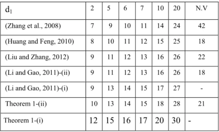
(25)For given d1={2,5,6, 7,10, 20} the maximum upper bounds d2
obtained by (Ramakrishnan and Ray, 2013) are {9,11,12,13,16,26}, while that of Theorem 1-(ii) gives larger delay bounds d2={12,15,16,17,20,30}, which means that the
proposed method is less conservative. Table 4 shows more results of the maximum bounds delay for different values of d1.
Table 4. Maximum bounds d2 for different value of d1. d1 2 5 6 7 10 20 N.V
(Zhang et al., 2008) 7 9 10 11 14 24 42 (Huang and Feng, 2010) 8 10 11 12 15 25 18 (Liu and Zhang, 2012) 9 11 12 13 16 26 22 (Li and Gao, 2011)-(ii) 9 11 12 13 16 26 18 (Li and Gao, 2011)-(i) 9 13 14 15 17 27 - Theorem 1-(ii) 10 13 14 15 18 28 21 Theorem 1-(i) 12 15 16 17 20 30 - It is clear that the results obtained in this paper are better than the existing one in the literatures. From the last column of Table 4 (N.V), we observe that the proposed method needs more decision variables than (Huang and Feng, 2010) and (Li and Gao, 2011)-(ii) and smaller variables than other methods
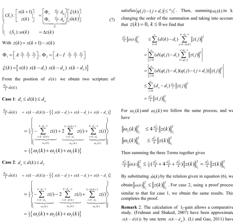
which means that the proposed method still effective and gives less conservative results. In other hand, Fig.1 describes the relationship of SSG condition 1
X G X
according to d1 when d2=8. From Fig.1 we can be seen that the SSG
condition obtained by our approach still smaller than other approximation based model used by other authors. This means that the proposed method is effective and less conservative.
Example 3. Consider the model of inverted pendulum system (Kwon et al., 2013), shown in Fig 5 with the following continuous description 3( ) 3 (4 ) (4 ) 0 1 0 ( ) ( ) 0 M m g l M m l M m x t u t (26) When M = 8kg, m = 2.0kg, l = 0.5m, g = 9.8m/s2 and
choosing sampling time Ts = 30ms, then system (26) can be
transformed to discrete-time system with the following parameters 1.00078 0.0301 0.0001 , 0.5202 1.0078 0.0005 A B
Fig. 5. Inverted pendulum system.
We consider this example to illustrate the advantages of the proposed method. When d1=1 and by applying Theorem 2
The maximum value of d2 which guarantees the asymptotic
stability of closed-loop system (20) is d2=8 for (K = K1 = K2)
and d2 > 15 for K1K2 while that of (Gao and Chen, 2007,
Kwon et al., 2013; Zhang et al., 2008; Huang and Feng, 2010) are 3,4,5,6 respectively. This means that our approach gives larger delay bounds.
Table 5 summaries study devoted to stabilization of system (20) and lists the maximum delay bounds and the controller gain obtained by other methods. The last column in Table 5 lists the number of iteration (N.Iter) satisfied Theorem 2 to be feasible.
CONTROL ENGINEERING AND APPLIED INFORMATICS 11
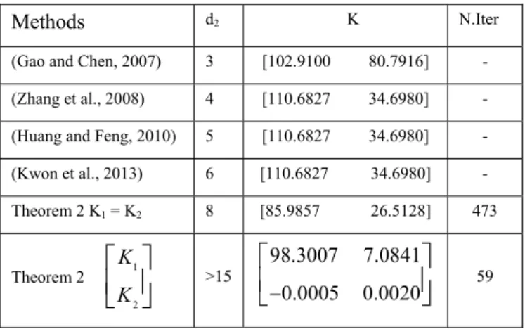
Table 5. Maximum bounds d2 and controller gains K.
Methods d2 K N.Iter
(Gao and Chen, 2007) 3 [102.9100 80.7916] - (Zhang et al., 2008) 4 [110.6827 34.6980] - (Huang and Feng, 2010) 5 [110.6827 34.6980] - (Kwon et al., 2013) 6 [110.6827 34.6980] - Theorem 2 K1 = K2 8 [85.9857 26.5128] 473 Theorem 2 1 2 K K
>15 98.3007 7.0841 0.0005 0.0020
59Firstly, it should be noted that Theorem 2 is satisfied with a small controller gain than those in (Gao and Chen, 2007; Zhang et al., 2008; Huang and Feng, 2010, Kwon et al., 2013). Moreover, the number of iteration needed to obtain feasible solution for K = K1 = K2 is 473, while that of
1 2
K K is 59, which means that the proposed method with
1 2
K K is better than (K = K1 = K2). The controller gains in
last line of Table 5 are obtained for given d1 = 1 and d2 = 15.
Fig 3 and Fig 4 plots the closed loop system using the controller gain (K = K1 = K2) and K1 K2respectively. Fig 3
shows that the state responses converge to zero for small time k, while that of Fig 4 needs more time k to approach zero. From this example we conclude that our method can control practical system with a smaller controller gain better than the existing methods in literature. Fig 3 and Fig 4 emphasize the merit of the proposed method. In the simulation, the initial values of the states are x(0) = [1;1] and time-delay d(k) is assumed as d k( ) 1 7 sin( k / 2)
1 8
5. CONCLUSION
In this paper, an improved delay-dependent stability for discrete-time linear systems has been developed. Based on a new model transformation performing a three-term approximation, stability criteria have been presented in term of a set of LMIs by using a direct Lyapunov-Krasovskii functional and SSG theorem. Thereafter, the problem of time-delayed controller design for discrete-time systems has been studied and a sufficient condition for the solvability of this problem has been given by using cone complementarity linearization (CCL) algorithms. It is better to mention that these results are extendable for filtering problem and for many types of systems. At the end, the proposed numerical examples have demonstrated the advantage of the method proposed to obtain less conservative results.
REFERENCES
Apkarian, P. and Gahinet, P. (1995). A convex characterization of gain-scheduled h controllers. IEEE
Transactions on Automatic Control., 40, 853-864. Chen, W.H., Guan, Z.H., and Lu, X. (2003). Delay-dependent
guaranteed cost control for uncertain discrete time
systems with delay. IEE Proceedings: Control Theory
and Applications., 150, 412-416.
Fridman, E. and Shaked, U. (2005). Stability and guaranteed cost control of uncertain discrete delay systems.
International Journal of Control., 78, 235-246.
Fridman, E. and Shaked, U. (2007). Input-output approach to stability and l2-gain analysis of systems with time-varying delays. Syst. Control Lett., 55, 1041-1053. Gao, H. and Chen, T. (2007). New results on stability of
discrete-time systems with time-varying state delay.
IEEE Transactions on Automatic Control., 52, 328-334. Gao, H., Lam, J., Wang, C., and Wang, Y. (2004). Delay-
dependent output-feedback stabilisation of discrete-time systems with time-varying state delay. IEE Proceedings:
Control Theory and Applications., 151, 691-698.
Ghaoui, L.E., Oustry, F., and Rami, A. (1997). A cone complementarity linearization algorithm for static output-feedback and related problems. IEEE Transactions on Automatic control., 42, 1171-1176. Gu, K., Zhang, Y., and Xu, S. (2011). Small gain problem in
coupled differential-difference equations, time-varying delays, and direct lyapunov method. Int. J. Robust
Nonlin. Control., 21, 429-451.
He, Y., Wang, Q.G., Lin, C., and Wu, M. (2007). Delay- range-dependent stability for systems with time-varying delay. Automatica., 43, 371-376.
Hmamed, A., El Aiss, H., and Hajjaji, A. (2015). Stability analysis of linear systems with time varying delay: An input output approach. IEEE 54th Annual Conference on
Decision and Control.
Huang, H. and Feng, G. (2010). Improved approach to delay-dependent stability analysis of discrete-time systems with time-varying delay. IET Control Theory Appl., 4, 2152-2159.
Huang, Y.P. and Zhou, K. (2000). Robust stability of uncertain time-delay systems. IEEE Trans. Autom.
Control., 45, 2169-2173.
Jiang, X., Han, Q.L., and Yu, X. (2005). Stability criteria for linear discrete-time systems with interval-like time-varying delay. Proceedings of the American Control
Conference., 2817-2822.
Kao, C.Y. and Lincoln, B. (2004). Simple stability criteria for systems with time-varying delays. Automatica., 40, 1429-1434.
Kao, C.Y. and Rantzer, A. (2007). Stability analysis of systems with uncertain time-varying delays. Automatica.,
43, 959-970.
Kim, J.H. (2011). Note on stability of linear systems with time-varying delay. Automatica, 47, 2118-2121.
Kwon, O.M., Park, M.J., Park, J.H., Lee, S.M., and Cha, E.J. (2013). Improved delay-dependent stability criteria for discrete-time systems with time-varying delays. Circuits
Syst Signal Process., 32, 1949-1962.
Lakshmanan, S., Senthilkumar, T., and Balasubramaniam, P. (2011). Improved results on robust stability of neutral systems with mixed time-varying delays and nonlinear perturbations. Appl. Math. Model, 35, 5355-5368. Li, X. and Gao, H. (2011). A new model transformation of
application to stability analysis. IEEE Transactions On
Automatic Control., 56.
Lin, C., Wang, Q.G., and Lee, T.H. (2006). A less conservative robust stability test for linear uncertain time delay systems. IEEE Transactions on Automatic
Control., 51, 87-91.
Liu, J. and Zhang, J. (2012). Note on stability of discrete-time discrete-time-varying delay systems. IET Control Theory
Appl., 6, 335-339.
Park, P. (1999). A delay-dependent stability criterion for systems with uncertain time-invariant delays. IEEE
Transactions on Automatic Control., 44, 876-877. Ramakrishnan, K. and Ray, G. (2013). Robust stability
criteria for a class of uncertain discrete-time systems with time-varying delay. Appl. Math. Model., 37, 1468-1479.
Shao, H. and Han, Q.L. (2011). New stability criteria for linear discrete-time systems with interval-like time-varying delays. IEEE Transactions On Automatic
Control., 56.
Su, X., Shi, P., WuA, L., and Song, Y.D. (2012). Novel approach to filter design for ts fuzzy discrete-time systems with time-varying delay. IEEE Transactions on
fuzzy systems., 20.
Sun, J., Liu, G., Chen, J., and Rees, D. (2010). Improved delay-range-dependent stability criteria for linear systems with time-varying delays. Automatica, 46, 466-470.
Xia, Y., Liu, G.P., Shi, P., Rees, D., and Thomas, E.J.C. (2007). New stability and stabilzation conditions for systems with time-delay. Int. J. Syst.Sci., 38, 17-24. Xu, S. and Lam, J. (2005). Improved delay-dependent
stability criteria for time-delay systems. IEEE
Transactions on Automatic Control., 50, 384-387. Xu, S. and Lam, J. (2008). A survey of linear matrix
inequality techniques in stability analysis of delay systems. Int. J. Syst. Sci., 39, 1095-1113.
Zhang, B., Xu, S., and Zou, Y. (2008). Improved stability criterion and its applications in delayed controller design for discrete-time systems. Automatica., 44, 2963-2967. Zhang, B., Zhou, S., and S.Xu (2007). Delay-dependent
Hinfinity controller design for linear neutral systems with
discrete and distributed delays. International Journal of
Systems Sciences., 38, 611-621.
Zhanga, J., Penga, C., and Zheng, M. (2015). Improved results for linear discrete-time systems with an intervaltime-varying input delay. International Journal
of Systems Science., 47, 492-499.
Zhao, L., Gao, H., and Karimi, H.R. (2013). Robust stability and stabilization of uncertain ts fuzzy systems with time-varying delay: An inputoutput approach. IEEE