HAL Id: cel-00392190
https://cel.archives-ouvertes.fr/cel-00392190
Submitted on 5 Jun 2009HAL is a multi-disciplinary open access archive for the deposit and dissemination of sci-entific research documents, whether they are pub-lished or not. The documents may come from teaching and research institutions in France or abroad, or from public or private research centers.
L’archive ouverte pluridisciplinaire HAL, est destinée au dépôt et à la diffusion de documents scientifiques de niveau recherche, publiés ou non, émanant des établissements d’enseignement et de recherche français ou étrangers, des laboratoires publics ou privés.
Numerical Analysis and Algorithms for Optimal Control
of Partial Differential Equations with Control and State
Constraints
Karl Kunisch
To cite this version:
Karl Kunisch. Numerical Analysis and Algorithms for Optimal Control of Partial Differential Equa-tions with Control and State Constraints. 3rd cycle. Castro Urdiales (Espagne), 2006, pp.159. �cel-00392190�
Numerical Analysis and Algorithms for
Optimal Control of Partial Differential
Equations with Control and State Constraints
Karl Kunisch
1July 28, 2006
1Institute of Mathematics and Scientific Computing, Karl-Franzens-Universit¨at
1
Model Problems and their Optimality
Sys-tems
The purpose of these notes is to introduce an approach for solving optimiza-tion problems which contain expressions which are Lipschitz continuous but not C1 by Newton-type methods. In spite of the lack of C1 regularity, ”high
rate” of convergence is our goal. More precisely we aim for a super-linear convergence.
In the remainder of this section we show by means of examples, where such problems arise in practice. Optimal control problems with control and state constraints are two of our generic model problems. The treatment of these problems here is infinite dimensional, i.e. we post these methods in properly chosen function spaces. Clearly for numerical realisation a disretisation is required. This is not addressed in these notes.
For each of the follwing problems we also state the first order optimality system. The derivation of these systems rely on Lagrange multiplier theo-rems. For convenience of the reader, we recall a prototype multiplier theorem in the Appendix of this section. The readers will notice that the regularity of the Lagrange multipliers, which are functional quantities in our cases, differ significantly from one problem to the other. These regularity properties have a tremendously strong influence on the proper numerical treatment.
Throughout these notes Ω denotes a bounded domain in Rn, with
bound-ary denoted by Γ or ∂Ω, assumed to be sufficiently smooth.
1.1
Optimal Control with Control Constraints
We consider the optimal control problem with distributed control u, state variable y and unilateral control constraints:
(P1) min J(y, u) = 1 2 Z Ω (y − z)2 dx +β 2 Z Ω u2 dx , (1.1) −∆y = u in Ω , y = 0 on Γ ,
(1.2) u ∈ L2(Ω) , u(x) ≤ ψ(x) for a.e. x ∈ Ω,
where z ∈ L2, β > 0 and , ψ ∈ L∞(Ω) .
For every u ∈ L2 system (1.1) has a unique solution y in H2 ∩ H1
0. It is
standard that problem (P1) has a unique solution (y∗, u∗) characterized by
the following optimality system : −∆y∗ = u∗ in Ω, y∗ ∈ H1 0(Ω), −∆p∗ = z − y∗ in Ω, p∗ ∈ H1 0(Ω), (βu∗− p∗, u − u∗) L2 ≥ 0 for all u ≤ ψ.
Here p∗ is referred to as the adjoint state. Let us give an equivalent
formulation for this optimality system which is essential to motivate the forthcoming algorithm:
Theorem 1.1. The unique solution (y∗, u∗) to problem (P1) is characterized
by (S) −∆y∗ = u∗ in Ω, y∗ ∈ H1 0(Ω) , −∆p∗ = z − y∗ in Ω, p∗ ∈ H1 0(Ω) , βu∗ = p∗− λ∗, λ∗ = c[u∗+ λ∗ c − Π(u ∗+λ∗ c )] = c max(0, u ∗+λ∗ c − ψ) , for every c > 0. Here Π denotes the projection of L2 onto U
ad = {u ∈ L2 :
u ≤ ψ}.
The proof can be given by inspection. Here and throughout, order re-lations like “max” and“ ≤ ”between elements of L2 are understood in the
pointwise almost everywhere sense.
We point out that the last equation in (S) (1.3) λ∗ = c[u∗+λ ∗ c − Π(u ∗ +λ∗ c )] is equivalent to (1.4) λ∗ ∈ ∂I Uad(u ∗) ,
where ∂IC denotes the subdifferential of the indicator function IC of a a
convex set C. This follows from general properties of convex functions (see 2
[IK1] for example) and can also easily be verified directly for the convex function IUad. The replacement of the well known differential inclusion (1.4)
in the optimality system for (P1) by (1.3) is an essential ingredient of the algorithm that we shall discuss.
It is also useful to consider the constraint u ≤ ψ in L2 in abstract terms,
expressing it as
G(u) = u − ψ ≤ 0, where G : L2 → L2.
Clearly G is surjective and hence existence of a Lagrange multiplier λ∗ in
L2 with the specified properties follows from abstract Lagrange multiplier
theory, c.f. the Appendix of the chapter.
Let us also note that (1.3) can be expressed as (1.5) λ∗ ≥ 0, u∗ ≤ ψ, (u∗− ψ)λ∗ = 0.
The ensemble of inequalities in (1.5) is called a complementarity system. Equation (1.3) is an equivalent formulation for (1.5) by means of nonlinear equation. In this context, the max operation is referred to as complementar-ity function.
For further treatment of (P1) we refer to [BIK], which is contained in these notes.
1.2
Obstacle Problems
We consider (P2) min 1 2 a(y, y) − (f, y) y ∈ H1 0(Ω) y ≤ ψ a.e. in Ω,where a (·, ·) is a bilinear form on H1
0(Ω) × H01(Ω) satisfying
(1.6) a(v, v) ≥ ν|v|2H1
0, a(w, z) ≤ µ|w|H1|z|H1,
for some ν > 0 and µ > 0 independently of v ∈ H1
0(Ω) and w, z ∈ H1(Ω). For example, (1.7) a(v, w) = Z Ω ∇v∇w dx 3
satisfies these requirements. Further it is assumed that f ∈ L2(Ω), ψ ∈ H1(Ω) with ψ|
∂Ω ≥ 0. Since ψ ∈ H1(Ω) the trace ψ|∂Ω is well-defined. The
assumption ψ|∂Ω ≥ 0 implies that the set of admissible functions y for (P2)
is nonempty. For our discussion the weak maximum principle, i.e. for all
v ∈ H1 0(Ω)
(1.8) a(v, v+) ≤ 0 implies v+ = 0,
where v+ = max(0, v), will be important. It is satisfied for (1.7)
It is standard to argue that P2 admits a unique solution y∗ ∈ H1 0(Ω).
From subsection 1.8, for example, it follows that there exists Lagrange mul-tiplier λ∗ ∈ H−1(Ω) associated to the inequality constraint y ≤ ψ. In fact,
G(y) = y − ψ, where G : H01 → H01
is surjective, so that the Lagrange multiplier is in (H1
0)∗ = H−1. Under
well-known regularity assumptions on the problem data it can be shown that the Lagrange multiplier satisfies additional regularity in the sense that
λ∗ ∈ L2(Ω), and that the following optimality system holds:
(1.9)
a(y∗, v) + (λ∗, v) = (f, v), for all v ∈ H1 0(Ω)
(λ∗, y∗− ψ) = 0, y∗ ≤ ψ, (λ∗, v) ≥ 0 for all v ∈ K,
where K = {v ∈ H1
0(Ω) : v ≥ 0 a.e.} and the inner products are taken in L2(Ω). By inspection (1.9) can equivalently be expressed as
(1.10)
a(y∗, v) + (λ∗, v) = (f, v) for all v ∈ H1 0(Ω) λ∗ = max(0, λ∗+ c(y∗− ψ)),
for arbitrary c > 0. (More precisely, (1.9) implies (1.10) for every c, and (1.10) for some c > 0 implies (1.9)). The extra Lagrange multiplier regu-larity does not follow from nonlinear programming arguments but rather by variational or pde techniques.
1.3
Optimal Control with State Constraints
This problem is related to P1 but the constraint acts on the state-variable rather than the control:
(P3) min J(y, u) = 1 2|y − z|2L2 + β2|u|2L2 subject to −∆y = u in Ω, y = 0 on ∂Ω, y ≤ ψ a.e. in Ω (y, u) ∈ H1 0(Ω) × L2(Ω),
where z ∈ L2(Ω), ψ ∈ C(Ω), ψ > 0 on ∂Ω and β > 0. It will be convenient
to set W = H1
0(Ω) ∩ H2(Ω). Under appropriate regularity requirements
every solutions to −∆y = u, with u ∈ L2(Ω) and y = 0 on ∂Ω satisfies y ∈ W ⊂ C(Ω), n ≤ 3. It is standard to argue the existence of a solution
(y∗, u∗) ∈ W ×L2(Ω) to (P3). It is also straightforward to argue the existence
of a Lagrange multiplier λ∗ ∈ W∗ since
G(y) = y − ψ, where G : W → W
is surjective. Let h·, ·iC∗,C denote the duality pairing between C(Ω) and its
topological dual C∗(Ω). The proof to the following characterization of the
solution to P3 with some extra regularity for the Lagrange multiplier is found in [BK], for example.
Theorem 1.2. The pair (y∗, u∗) ∈ W × L2(Ω) is a solution to (P) if and only if there exists p∗ ∈ L2(Ω) and λ∗ ∈ C∗(Ω) such that
−∆y∗ = u∗ in Ω, y∗ = 0 on ∂Ω, (p∗, −∆y) + hλ∗, yi C∗,C = (z − y∗, y) for all y ∈ W βu∗ = p∗ y∗ ≤ ψ, hλ∗, y∗− ψi C∗,C = 0, hλ∗, yi
C∗,C ≥ 0, for all y ∈ C(Ω) with y ≥ 0.
In general the regularity of λ∗ is no better than specified in Theorem1.2.
In fact if the active set at the solution
A = {x : y∗(x) = ψ(x)}
is a connected domain in Ω then it can be shown that λ∗ = λ∗
d+ λ∗b, where
λ∗
d∈ L2(Ω) and λ∗b ∈ L2(∂A). In particular λ∗ in not in L2(Ω) in general.
1.4
L
1and BV Functionals
In recent years, the space BV ( functions of total bounded variation) and of the use of L1 functionals receives a considerable amount of attention. We
consider two such cases here.
The relationship to the previous subsection stems from the fact that in-dicator functions ( describing the inequality constraints) and norm functions are dual to each other in the sense of Fenchel duality.
We consider the image denoising problem with L1-fitting and smooth
regularization (P4) min u∈H1 0(Ω) Z Ω · β 2|∇u| 2+ |u − z| ¸ dx
for the given function z ∈ L1(Ω). Note that the cost functional in (P4) is
nondifferentiable in the classical sense. We see that problem (P4) is equiva-lent to (1.11) min u∈H1 0(Ω) max λ∈C Z Ω · β 2|∇u| 2+ λ(u − z) ¸ dx = min u∈H1 0(Ω) max λ∈C l(u, λ), where l : H1
0(Ω) × L2(Ω) → R is the Lagrange-functional and the set C is
defined as
C := ©λ ∈ L2(Ω) : |λ(x)| ≤ 1 a.e. x ∈ Ωª.
The equivalence of the two formulations results from the following identity max λ∈C Z Ω λ(u − z) dx = Z Ω |u − z| dx.
Hence, λ represents the Lagrange smoothing of the subdifferential sign(u−z) [IK1].
The ptimality conditions for the solution u∗ is formally easily found to be (1.12) −β ∆u∗+ λ∗ = 0, in Ω, λ∗(x) = λ∗(x) + c (u∗− z)(x)
max{1, |λ∗(x) + c (u∗− z)(x)|}, a. e. x ∈ Ω, for each c > 0.
The second condition realizing the complementarity condition is equivalent to the actual definition of the subdifferential
(1.13) λ
∗(x) = (u∗− z)(x)
|(u∗− z)(x)|, in I
∗(x) = {x ∈ Ω | (u∗− z)(x) 6= 0} ,
|λ∗(x)| ≤ 1, in J∗(x) = {x ∈ Ω | (u∗− z)(x) = 0} .
From the optimality conditions it follows that u∗ ∈ H2.
The corresponding image denoising problem with quadratic L2-fitting
reads as (1.14) min u∈H1 0(Ω) Z Ω · β 2|∇u| 2+ |u − z|2 ¸ dx
with the linear optimality condition
(1.15) −β∆˜u∗+ 2 (˜u∗ − z) = 0
for the unique solution ˜u∗. Comparing (1.15) to (1.12) and (1.13), one
no-tices that for the L2-formulation the distance between ˜u∗ and z plays an
important role in the optimality condition (1.15), whereas only the (regu-larized) sign-function for (u∗ − z) appears in (1.12). This illustrates the
relative insensitivity of the L1-formulation towards outliers compared to
the L2-formulation.
We recall the Fenchel duality theorem in infinite dimensional spaces in a form that is convenient here. Let V and Y be Banach spaces with topological duals denoted by V∗ and Y∗, respectively. Further let Λ ∈ L(V, Y ) and let
F : V → R ∪ {∞}, G : Y → R ∪ {∞} be convex, lower semi-continuous
functionals not identically equal to ∞, and assume that there exists v0 ∈ V
such that F(v0) < ∞, G(Λv0) < ∞ and G is continuous at Λv0. Then we
have
(1.16) inf
u∈V F(u) + G(Λu) = supp∈V∗−F
∗(Λ∗p) − G∗(−p),
where F∗ : V∗ → R ∪ {∞} denotes the conjugate of F defined by
F∗(v∗) = sup
v∈Vhv, v ∗i
V,V∗ − F(v).
Under the conditions imposed on F and G it is known that the problem on the right hand side of (1.16) admits a solution. Moreover, (¯u, ¯p) are solutions
to the two optimization problems in (1.16) if and only if Λ∗p ∈ ∂F(¯¯ u),
(1.17a)
−¯p ∈ ∂G(Λ¯u),
(1.17b)
where ∂F denotes the subdifferential of the convex functional F.
Using the Fenchel duality theorem the dual of (P4) is formally found to be (1.18) min p∈L2(Ω)2F ∗(−div p) + 1 2β Z Ω |p|2, where F∗(v) = ½ ∞, |v| > 1 vz, |v| ≤ 1. .
The relation between the solution to (1.18) and P4 is given by
p∗ = −β∇u∗
.
A typical image reconstruction problem based on the BV semi-norm is given by (P5) ( min 1 2 R Ω|Ku − f |2dx +α2 R Ω|u|2dx + β R Ω|Du| over u ∈ BV,
where β > 0, α ≥ 0 are given and K ∈ L(L2(Ω)). We assume that constant functions are not in the kernel of K or α > 0. Further BV(Ω) denotes the space of functions of bounded variation. A function u is in BV(Ω) if the BV semi-norm defined by Z Ω |Du| = sup ½Z Ω u div ~v : ~v ∈ (C∞ 0 (Ω))2, |~v(x)|`∞ ≤ 1 ¾ 8
is finite.
The great advantage of BV-regularization over regularization involving
|∇u|2 lies in the fact that the former perserves corners and edges in the
image significantly better than the latter.
Formally ( as a reasonably simple exercise) the Fenchel dual of this prob-lem is found to be:
(1.19) ( inf 1 2| div ~p + K∗f |2B s.t. − β~1 ≤ ~p(x) ≤ β~1 for a.e. x ∈ Ω, where |v|2
B= (v, B−1v), and the relationship between solutions to the original
and the dual problem is given by
(1.20) div ~p = Bu − K∗f, ~p = β ∇u
|∇u| on {x : ∇u(x) 6= 0}.
Note that (1.19) is a bilaterally constrained optimization problem. Rigorously we have the following result, where H0(div) = {~v ∈ IL2(Ω) :
div ~v ∈ L2(Ω), ~v · n = 0 on ∂Ω}, and n is the outer normal to ∂Ω. Theorem 1.3. Consider the problem
(1.21)
(
min 1
2| div ~p + K∗f |2B for ~p ∈ H0(div) s.t. − β~1 ≤ ~p ≤ β~1,
Its dual is given by (P5).
1.5
Miscellanies
There are still many related problems of non-differentiable optimization prob-lems in function spaces, for example friction and contact probprob-lems and Bing-ham fluid problems (two phase fluids).
Interesting and, in part open problems, are related to considering opti-mization problems subject to variational inequalities, as treated in 1.3 as constraints. Such problems are referred to as control of variational inequal-ities. Equally interesting are problems, where the obstacle itself acts as a control. From the point of view of mathematical programming all these problems are nested complementarity problems in function spaces.
1.6
Comments on the attached papers,[BIK, HIK, IK3,
IK5, HK2]
Let me give a short introduction to the five selected papers which are attached to this file.
In [BIK] the primal dual active set strategy for solving control constrained optimal control problems is introduced and some global convergence proper-ties are obtained. The starting point for this algorithm is the last equation in (S):
λ∗ = max(0, λ∗+ c(u∗− ψ)
. In the course of an iterative algorithm we decide, at iteration-level k to define the updated ’active’ set to be
Ak = {x : λk+ c(uk− ψ) > 0}.
In the following iteration the control is fixed to be ψ on Ak, and is considered
unconstrained on the inactive set Ik= Ω \ Ak. We ask the readers, who just
want to glimpse into these notes to read sections 1 and 2 of [BIK]. The primal-dual active set strategy may appear to be a fixed point iteration - but this would be the wrong way to think of it. In fact, it is a Newton method, where the max-operation is teated as if it was differentiable.
While the max-operation is not differentiable in the classical sense, it is Newton-differentiable, as operator between appropriate spaces, as de-scribed in [HIK]. Actually, Newton-differentiable is called ’slant-differentiability’ in [HIK], for reason that I will explain in the course. Suffice it to say here that Newton differentiability implies local super-linear convergence of the Newton algorithm. Moreover, it is shown in [HIK] that the primal dual ac-tive set strategy is equivalent to a Newton step (we now call it ’semi-smooth’ Newton step), applied to the max-operation. In [HIK] it is shown that max is Newton differentiable between finite-dimensional spaces, and as operator between Lp and Lq, provided that q < p. Looking back over the examples
in subsections 1.1.-1.4. we need to address the question, when this case of Newton-differentiability occurs. It holds, for quite generally for control con-strained optimal control problems. This is also covered in [HIK]. But it is not true generically. ( We ask the readers not to skip too much from [HIK].) In [IK3] we focus on the semi-smooth Newton method for obstacle-type problems, as considered in section 1.2 above. Recall, that this is the case where the Lagrange multiplier has L2 regularity, but this does not follow
di-rectly from a Lagrange multiplier theorem. We define a family of regularized 10
problems which are semi-smooth and which converge to the original problem asymptotically. Moreover we analyse monotonicity type problems, which are related to the weak maximum principle, satisfied by this class of examples -or the M-matrix property, if properly discretized. I ask the readers to read the theorems - the proofs are not essential for what follows.
In [IK5] we treat the even less regular case of state constrained optimal control problems. Here the Lagrange multipliers are generically not L2, but
rather only measures. Again we introduce a family of approximating prob-lems which are semi-smooth, and which converge to the original problem asymptotically. The reader may want to consider the numerical section in both [IK3] and [IK5] and note that , if we knew how to tune the parameter, which defines the regularization, and let it tend to infinity in a clever way, then this would be very efficient.
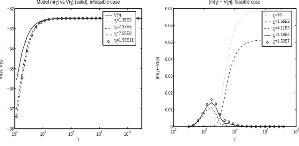
This point is also addressed in [HK1]. We introduce a ”path” which describes the behavior of the regularized problems as a function of the regu-larization parameter. Mathematically the path is a consequence of sensitivity analysis. Intuitively we may think that on the path the problems are better behaved than far off the path. - But of course this path is not available to us quantitatively. However, some intricate manipulations allow to get models for the path on the basis of just two evaluations of the regularized problems with two different regularization parameters. On the basis of these models an approximate path is available, and strategies can be developed for systematically updating the regularization parameter.
1.7
Appendix: A Lagrange Multiplier Theorem
To derive first order necessary optimality conditions for constrained optimiza-tion problems the following Lagrange multiplier theorem is useful, c.f.[C]. Below DG denotes the Gateaux differential of the mapping G. By definition the Gateaux derivative is a continuous linear mapping.
Theorem 1.4. Let U and Z be Banach spaces, and K ⊂ U, C ⊂ Z be
convex subsets, with C having a nonempty interior. Let ¯u ∈ K ba a solution of the optimization problem
½
min J(u),
u ∈ K, G(u) ∈ C,
where J : U → (−∞, ∞] and G : U → Z are two Gateaux differentiable
mappings at ¯u. Then there exist a real number ¯µ ≥ 0 and an element ¯λ ∈ Z∗
such that
¯
µ + |¯λ|Z∗ > 0,
h¯λ, z − G(¯u)i ≤ 0, for all z ∈ C,
h¯µJ0(¯u) + [DG(¯u)]∗λ, u − ¯¯ ui ≥ 0 for all u ∈ K.
Moreover, ¯µ can be taken equal to 1 if the following condition of Slater type is satisfied:
there exists u0 ∈ K such that G(¯u) + DG(¯u)(u0− ¯u) ∈ int C.
References
[BHHK] M. BERGOUNIOUX, M. HADDOU, M. HINTERM ¨ULLER and K. KUNISCH: A Comparison of a Moreau-Yosida Based Active Strategy and Interior Point Methods for Constrained Optimal Control Problems, SIAM J. on Optimization, 11(2000), 495–521.
[BIK] M. BERGOUNIOUX, K. ITO and K. KUNISCH: Primal-dual Strat-egy for Constrained Optimal Control Problems, SIAM J. Control and Optimization, 37(1999), 1176–1194.
[BK] M. BERGOUNIOUX und K. KUNISCH: On the Structure of the La-grange Multiplier for State-Constrained Optimal Control Problems, Sys-tems and Control Letters, 48(2002), 16-176.
[C] E. Casas: Boundary Control of Semilinear Elliptic Equations with Point-wise State Contraints, SIAM J. Control and Optim., 31(1993), 993-1006. [DK1] J. C. de los REYES and K. KUNISCH: A semi-smooth Newton method for control constrained optimal control of the Navier Stokes equations, Nonlinear Analysis, 62(2005),1289-1316.
[DK2] J. C. de los REYES and K. KUNISCH: A comparison of algorithms for control constrained optimal control of the Burgers equation, 41(2004), 203-225.
[HHKOS] W. HINTERBERGER, M. HINTERM ¨ULLER, K. KUNISCH, M. v. OEHSEN and O. SCHERZER: Tube methods for BV regular-ization, J. Math. Imaging and Vision, 19(2003), 219-236.
[HIK] M. HINTERM ¨ULLER, K. ITO and K. KUNISCH: The primal–dual active set strategy as a semi–smooth Newton method, SIAM Journal on Optimization, 13(2002), 865-888.
[HK1] M. HINTERM ¨ULLER and K. KUNISCH: Total bounded variation regularization as bilaterally constrained optimization problem, SIAM J. Appl. Mathematics 64(2004), 1311-1333.
[HK2] M. HINTERM ¨ULLER and K. KUNISCH: Path-following methods for a class of constrained minimization problems in function space, to appear in SIAM J. on Optimization.
[IK1] K. ITO and K. KUNISCH: Augmented Lagrangian Methods for Nons-mooth Convex Optimization in Hilbert Spaces, Nonlinear Analysis, The-ory, Methods and Applications, 41(2000), 591–616.
[IK2] K. ITO and K. KUNISCH: Optimal Control of Elliptic Variational Inequalities, Applied Mathematics and Optimization, 41(2000), 343– 364.
[IK3] K. ITO and K. KUNISCH: Semi-smooth Newton methods for varia-tional inequalities of the first kind, Mathematical Modelling and Nu-merical Analysis, 37(2002), 41-62.
[IK4] K. ITO and K. KUNISCH: The primal-dual active set method for nonlinear optimal control problems with bilateral constraints, SIAM J. on Control and Optimization, 43(2004), 357-376.
[IK5] K. ITO and K. KUNISCH: Semi-smooth Newton methods for state-constrained optimal control problems, Systems and Control Letters, 50(2003), 221-228.
[IK6] K. ITO and K. KUNISCH: Parabolic variational inequalities: the Lan-grange multiplier approach, Journal de Math. Pures et Appl., to appear. bibitem[IK7]IK7 K. ITO and K. KUNISCH: Optimal Control of Obsta-cle Problems by H1-Obstacles, Appl. Math. and Optim., to appear.
[KKM] T. K ¨ARKK ¨AINEN, K. KUNISCH and K. MAJAVA: Denoising using L1-fitting, Computing, 74(2005), 353-376.
[KKT] T. KARKKAINEN, K. KUNISCH und P. TARVAINEN: Primal-Dual Active set Methods for Obstacle Problems, J. Optimization Theory and Appl., 119(2003), 499-533.
[KRe] K. KUNISCH and F. RENDL: An Infeasible Active Set Method for Quadratic Problems with Simple Bounds, SIAM Journal on Optimiza-tion, 14(2003), 35-52.
[KRo] K. KUNISCH and A. R ¨OSCH: Primal-dual active set strategy for a general class of constrained optimal control problems, SIAM Journal on Optimization, 13(2002), 321-334.
[KS] K. KUNISCH and G. STADLER: Generalized Newton methods for the 2D-Signorini contact problem with friction in function space, ESIAM: M2AN, 39(2005), 827-854.
Primal-dual Strategy for Constrained Optimal Control
Problems
ma¨ıtine bergounioux1 kazufumi ito2 karl kunisch3
Abstract
An algorithm for efficient solution of control constrained optimal control problems is proposed and analyzed. It is based on an active set strategy involving primal as well as dual variables. For discretized problems sufficient conditions for convergence in finitely many iterations are given. Numerical examples are given and the role of strict complementarity condition is discussed.
Keywords: Active Set, Augmented Lagrangian, Primal-dual method, Optimal Control. AMS subject classification. 49J20, 49M29
1
Introduction and formulation of the problem
In the recent past significant advances have been made in solving efficiently nonlinear optimal control problems. Most of the proposed methods are based on variations of the sequential quadratic programming (SQP) technique, see for instance [HT, KeS, KuS, K, T] and the references given there. The SQP-algorithm is sequential and each of its iterations requires the solution of a quadratic minimization problem subject to linearized constraints. If these auxiliary problems contain inequality constraints with infinite dimensional image space then their solution is still a significant challenge.
In this paper we propose an algorithm for the solution of infinite dimensional quadratic problems with linear equality constraints and pointwise affine inequality constraints. It is based on an active set strategy involving primal and dual variables. It thus differs signifi-cantly from conventional active set strategies that involve primal variables only, see [Sch] for example. In practice the proposed algorithm behaves like an infeasible one. The iterates of
1UMR-CNRS 6628, Universit´e d’Orl´eans, U.F.R. Sciences, B.P. 6759, F-45067 Orl´eans Cedex 2, France.
E-mail: [email protected]. This work was supported in part by EEC, HCM Contract CHRX-CT94-0471
2Department of Mathematics, North Carolina State University, Raleigh, NC27695, USA.
3Institut f¨ur Mathematik, Universit¨at Graz, A-8010 Graz, Austria, E-mail: [email protected]. Work
supported in part by EEC, HCM Contract CHRX-CT94-0471 and Fonds zur F¨orderung der wissenschaftlichen Forschung, UF8,“Optimization and Control”.
the algorithm violate the constraints up to the next-to-the-last iterate. The algorithm stops at a feasible and optimal solution.
Within this paper we do not aim for generality but rather we treat as a model problem an unilateral control constraint optimal control problem related to elliptic partial differential equations. The distributed nature of this problem, which is reflected in the fact that it behaves like an obstacle problem for the biharmonic equation, makes it difficult to analyze.
Let us briefly outline the contents of the paper. The algorithm will be presented in Section 2. We prove that if the algorithm produces the same active set in two consecutive iterates then the optimal solution has been obtained. In Section 3 we shall give sufficient conditions which guarantee that an augmented Lagrangian functional behaves as a decreasing merit function for the algorithm. In practice this implies finite step convergence of the discretized problem. Section 4 is devoted to showing that for a minor modification of the algorithm the cost functional is increasing until the feasible optimal solution is reached. In Section 5 several numerical examples are given. For most examples the algorithm behaves extremely efficient and typically converges in less than five iterations. Thus, to present interesting cases the majority of the test examples is in some sense extreme: Either the strict complementarity condition is violated or the cost of the control is nearly zero.
To describe the problem, let Ω be an open, bounded subset of RN , N ≤ 3, with smooth
boundary Γ and consider the following distributed optimal control problem :
min J(y, u) = 1 2 Z Ω (y − zd)2 dx + α 2 Z Ω (u − ud)2 dx , (P) −∆y = u in Ω , y = 0 on Γ , (1.1) u ∈ Uad ⊂ L2(Ω) , (1.2)
where zd, ud∈ L2(Ω), α > 0 and Uad = { u ∈ L2(Ω) | u(x) ≤ b(x) a.e. in Ω}, b ∈ L∞(Ω) .
It is well known that, for every u ∈ L2(Ω) system (1.1) has a unique solution y = T (u) in
H2(Ω) ∩ Ho1(Ω).
Remark 1.1 To emphasis the basic ideas of the proposed approach we treated the rather
simple problem (P). Many generalizations are possible. In particular, −∆ in (1.1) can be replaced by any strictly elliptic second order differential operator.
It is standard that problem (P) has a unique solution (y∗, u∗) characterized by the
fol-lowing optimality system : −∆y∗ = u∗ in Ω, y∗∈ H1 o(Ω) , −∆p∗= zd− y∗ in Ω, p∗∈ Ho1(Ω) , (α(u∗− u d) − p∗, u − u∗) ≥ 0 for all u ∈ Uad, 2
where (·, ·) denotes the L2(Ω)-inner product.
Let us give an equivalent formulation for this optimality system which is essential to motivate the forthcoming algorithm:
Theorem 1.1 The unique solution (y∗, u∗) to problem (P) is characterized by
(S) −∆y∗= u∗ in Ω, y∗ ∈ H1 o(Ω) , −∆p∗ = zd− y∗ in Ω, p∗∈ Ho1(Ω) , u∗ = ud+p∗− λ∗ α , λ∗ = c[u∗+λ∗ c − Π(u ∗+λ∗ c )] = c max(0, u ∗+λ∗ c − b) ,
for every c > 0. Here Π denotes the projection of L2(Ω) onto U
ad. Proof - We refer to [IK].
We point out that the last equation in (S)
λ∗ = c[u∗+λ ∗ c − Π(u ∗+λ∗ c )] (1.3) is equivalent to λ∗ ∈ ∂IUad(u ∗) , (1.4)
where ∂IC denotes the subdifferential of the indicator function IC of a a convex set C. This follows from general properties of convex functions (see [IK] for example) and can also easily be verified directly for the convex function IUad. The replacement of the well
known differential inclusion (1.4) [B] in the optimality system for (P) by (1.3) is an essential ingredient of the algorithm that we shall propose.
Here and below, order relations like “max” and“ ≤ ”between elements of L2(Ω) are
understood in the pointwise almost everywhere sense.
Let us interpret the optimality system (S). From −∆y∗= ud+p∗− λ∗
α it follows that p∗= α[−∆y∗− u d] + λ∗ and hence −α∆y∗− ∆−1y∗+ λ∗= α ud− ∆−1zd. It follows that αu∗+ ∆−2u∗+ λ∗ = αu d− ∆−1zd , λ∗ = c max(0, u∗+λ∗ c − b) for all c > 0
which implies the highly distributed nature of the optimal control. Setting H = αI + ∆−2
and f = αud− ∆−1z
d, system (S) can be expressed as
(S)1 Hu∗+ λ∗ = f , λ∗ = c max(0, u∗+λ ∗ c − b) for all c > 0 3
We observe that by setting u = −∆y, system (S) constitutes an optimality system for the variational inequality min α 2 Z Ω |∆y|2dx + 1 2 Z Ω |y − (zd− α ∆ud)|2dx y ∈ H1 o(Ω) ∩ H2(Ω) −∆y ≤ b
the regularity of which was studied in [BS].
2
Presentation of the Algorithm
In this section we present the primal-dual active set algorithm and discuss some of its basic properties. Let us introduce the active and inactive sets for the solution to (P) and define
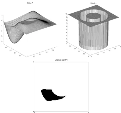
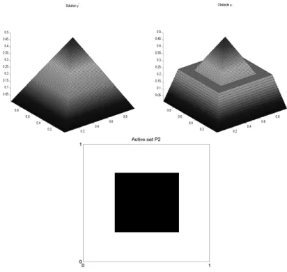
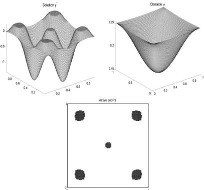
A∗ = { x | u∗(x) = b a.e. } and I∗ = { x | u∗(x) < b a.e. } .
The proposed strategy is based on (1.3). Given (un−1, λn−1) the active set for the current
iterate is chosen as
An= { x | un−1(x) + λn−1(x)
c > b a.e. } .
We recall that λ∗ ≥ 0 and in the case of strict complementarity λ∗ > 0 on A∗. The complete algorithm is specified next
Algorithm 1. Initialization : choose yo, uo and λo and set n = 1.
2. Determine the following subsets of Ω :
An= { x | un−1(x) + λn−1c(x) > b } , In= { x | un−1(x) + λn−1c(x) ≤ b } .
3. If n ≥ 2 and An= An−1 then stop.
4. Else, find (yn, pn) ∈ H1 o(Ω) × Ho1(Ω) such that −∆yn= b in An ud+pαn in In , −∆pn= zd− yn in Ω . and set un= b in An ud+pαn in In , 4
5. Set λn= pn− α(un− ud), update n = n + 1 and goto 2.
The existence of the triple (yn, un, pn) satisfying the system of step 4 of the Algorithm
follows from the fact that it constitutes the optimality system for the auxiliary problem (Paux) min { J(y, u) | y ∈ Ho1(Ω), − ∆y = u in Ω, u = b on An}
which has (yn, un) as unique solution.
We may use different initialization schemes. The one that was used most frequently is the following one:
uo = b , −∆yo= uo, yo∈ Ho1(Ω) , −∆po= zd− yo , po ∈ Ho1(Ω) , λo= max(0, α(ud− b) + po) . (2.1)
This choice of initialization has the property of feasibility. Alternatively, we tested the algorithm with initialization as the solution of the unconstrained problem, i.e.
λo = 0 −∆yo = ud+ po α , yo ∈ Ho1(Ω) , −∆po = zd− yo , po∈ Ho1(Ω) , uo= ud+po α . (2.2)
For all examples the first initialization behaved better or equal to the second.
The initialization process (2.1) has the property that the first set A1 is always included in
the active set A∗ of problem (P). More precisely we have
Lemma 2.1 If (uo, yo, λo) are given by (2.1) with uo≥ u∗; then λo≤ λ∗.
In addition, if uo = b then A1 ⊂ A∗.
Proof - By construction
λo= max(0, α(ud− uo) + po) = max(0, α(ud− uo) + ∆−1(yo− zd)) ,
and as a consequence of (S)
λ∗ = α(ud− u∗) + p∗= α(ud− u∗) + ∆−1(y∗− zd) = α(ud− u∗) − ∆−2u∗− ∆−1zd ≥ 0.
It follows that
λ∗− λo= λ∗ ≥ 0 if α(ud− uo) + ∆−1(yo− zd) ≤ 0 , and
λ∗− λ
o= α(uo− u∗) + ∆−2(uo− u∗) + α(ud− uo) + ∆−1(yo− zd) else .
If uo≥ u∗ the maximum principle yields ∆−2(uo− u∗) ≥ 0 and λ∗− λo ( = λ∗ ≥ 0 if α(ud− uo) + ∆−1(yo− zd) ≤ 0 ≥ α(ud− uo) + ∆−1(yo− zd) ≥ 0 else . Therefore λo ≤ λ∗.
In addition, if uo = b then uo+λco = b +λco > b on A1. Consequently λo > 0 on A1 and
λ∗ > 0. It follows that A
1 ⊂ A∗ and the proof is complete.
A first convergence result which also justifies the stopping criterion in Step 3 is given in the following theorem.
Theorem 2.1 If there exists n ∈ N − {0} such that An= An+1 then the algorithm stops and the last iterate satisfies
(Sn) −∆yn= un= b in An ud+pn α in Ω − An , −∆pn= zd− yn in Ω . λn= pn− α(un− ud) , un∈ Uad with λn= 0 on In and λn> 0 on An . (2.3)
Therefore, the last iterate is the solution of the original optimality system (S).
Proof - If there exists n ∈ N − {0} such that An= An+1, then it is clear that algorithm stops
and the last iterate satisfies (Sn) by construction except possibly for un∈ Uad. Thus we have to prove un∈ Uad and (2.3).
• On In we have λn= 0 by step 5 of the Algorithm. Moreover un+λcn = un≤ b, since
In= In+1.
• On An we get un = b and un+ λcn > b since An= An+1.Therefore λn > 0 on An and
un∈ Uad.
To prove that the last iterate is a solution of the original optimality system (S), it remains to show that
λn= c[un+λcn − Π(un+λcn)] .
• On In we have λn= 0 and un+λcn = un≤ b. It follows that
un+λn
c − Π(un+
λn
c ) = un− Π(un) = 0 = λn .
• On An we get un= b, λn> 0 and therefore c[un+λn c − Π(un+ λn c )] = c[b + λn c − b] = λn .
Now we give a structural property of the algorithm :
Lemma 2.2 If un is feasible for some n ∈ N − {0} (i.e. un≤ b) then An+1⊂ An .
Proof - On Inwe get λn= 0 by construction, so that un+λcn = un≤ b (because of feasibility).
This implies In⊂ In+1 and consequently An+1 ⊂ An .
Note that Theorem 2.1 and in particular (2.3) does not utilize or imply strict complemen-tarity. In fact, if (2.3) holds, then the set of x for which un(x) = b and λn(x) = 0 is contained in In.
We end this section with “simple cases” where we may conclude easily that the algorithm is convergent.
Theorem 2.2 For initialization (2.1), the Algorithm converges in one iteration in the
fol-lowing cases
1. zd≤ 0, ud= 0 , b ≥ 0 and the solution to −α∆u − ∆−1u = zd is nonpositive.
2. zd≥ 0, b ≤ 0, ud> b or
zd≥ 0, b ≤ 0, ud≥ b and zd+ ∆−1b is not zero as element in L2(Ω).
Proof - Let us first examine case 1. The maximum principle implies that −∆−1u
o ≥ 0 .
Consequently zd+ ∆−1uo≤ 0 and by a second application of the maximum principle −∆−1(zd+ ∆−1uo) ≤ 0 .
Together with the fact that ud− b = −b ≤ 0, this implies
λo = max(0, α(ud− b) − ∆−1(zd+ ∆−1uo)) = 0 . Therefore A1= ∅ and I1 = Ω.
Using the first iteration we obtain u1= pα1 in Ω. Moreover −∆y1= u1 and −∆p1 = zd− y1
imply that
−α∆u1− ∆−1u1= zd .
By assumption u1 is feasible. Therefore A2 = A1 = ∅ and by Theorem 2.1 the algorithm
stops at the solution to (P).
Now we consider case 2. By assumption and due to (2.1) we have zd≥ 0, b ≤ 0 , λo≥ 0 and A1= { λo> 0 }. Due to the maximum principle −∆−1u
o≤ 0 and
po = −∆−1(zd− yo) = −∆−1[zd− (−∆−1uo)] ≥ 0 .
Moreover if zd+ ∆−1b is not the zero element in L2(Ω), then p
o> 0 in Ω and α(ud− b) + po >
α(ud− b).
If ud > b or (ud = b and zd+ ∆−1b 6= 0) then λo = max(0, α(ud− b) + po) > 0 in Ω ( and
λo = 0 on ∂Ω). Consequently A1 = Ω and u1 = b, λ1 = −∆−1(z
d+ ∆−1b) + α(ud− b) > 0.
This yields A2 = A1 = Ω and the algorithm stops.
3
Convergence analysis
3.1 The Continuous Case
The convergence analysis of the Algorithm is based on the decrease of appropriately chosen merit functions. For that purpose we define the following augmented Lagrangian functions
Lc(y, u, λ) = J(y, u) + (λ, ˆgc(u, λ)) +c2kˆgc(u, λ)k2 and ˆLc(y, u, λ) = Lc(y, u, λ+) ,
where (·, ·) is the L2(Ω)-inner product, k·k is the L2(Ω)-norm, λ+= max(λ, 0) and ˆg
c(u, λ) =
max(g(u), −λ
c) with g(u) = u − b. Further (·, ·)|S and k · k|S denote the L2-inner product and
norm on a measurable subset S ⊂ Ω. Note that the mapping
u 7→ (λ, ˆgc(u, λ)) +2ckˆgc(u, λ)k2 ,
is C1, which is not the case for the function given by
u 7→ (λ, g(u)) + c
2k max(g(u), 0)k
2 .
The following relationship between primal and dual variables will be essential. Lemma 3.1 For all n ∈ N − {0} and (y, u) ∈ H1
o(Ω) × L2(Ω) satisfying −∆y = u we have J(yn, un) − J(y, u) = −12ky − ynk2−α2ku − unk2+ (λn, u − un)|An (3.1)
Proof - Using kak2− kbk2= −ka − bk2+ 2 (a − b, a) and Steps 4 and 5 of the Algorithm, we
find that J(yn, un) − J(y, u) = −12ky − ynk2−α2ku − unk2+ (yn− y, yn− zd) + α (un− u, un− ud) = −1 2ky − ynk 2−α 2ku − unk 2+ (∆(y n− y), pn) + α (un− u, un− ud) = −1 2ky − ynk 2−α 2ku − unk 2+ (u n− u, −pn+ α(un− ud)) = −1 2ky − ynk 2− α 2ku − unk 2+ (u − u n, λn) .
As λn= 0 on In the result follows.
Let us define
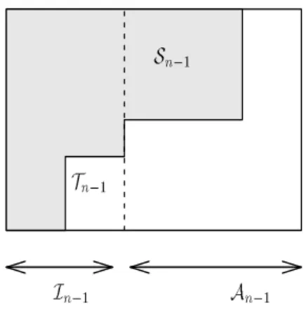
Sn−1= { x ∈ An−1 | λn−1(x) ≤ 0 } and Tn−1= { x ∈ In−1 | un−1(x) > b(x) } .
These two sets can be paraphrased by calling Sn−1 the set of elements that the active set
strategy predicts to be active at level n − 1 but the Lagrange multiplier indicates that they should be inactive, and by calling Tn−1 the set of elements that was predicted to be inactive
but the n − 1st iteration level corrects it to be active. We note that
Ω = (In−1\Tn−1) ∪ Tn−1∪ Sn−1∪ (An−1\Sn−1) (3.2)
defines a decomposition of Ω in mutually disjoint sets. Moreover we have the following relation between these sets at each level n:
In= (In−1\Tn−1) ∪ Sn−1 , An= (An−1\Sn−1) ∪ Tn−1 . (3.3)
In fact, as Ω = In∪ An is is sufficient to prove that
(In−1\Tn−1) ∪ Sn−1⊂ In and (An−1\Sn−1) ∪ Tn−1⊂ An ,
that is
Sn−1⊂ In and Tn−1 ⊂ An .
Since Sn−1⊂ An−1 we find un−1= b on Sn−1. From the definition of Sn−1 we conclude that
λn−1≤ 0 so that un−1+λn−1
c ≤ b. This implies Sn−1⊂ In. The verification of Tn−1⊂ An
is quite similar.
For the convenience of the reader we present these sets in Figure 1.
I n 1 A n 1 T n 1 S n 1
Figure 1: Decomposition of Ω at levels n − 1 and n
In Figure 1 the shaded region depicts In and the white region is An. The following table
depicts the signs of primal and dual variables for two consecutive iteration levels.
λn−1 λn un−1 un Tn−1= In−1∩ An 0 > b = b Sn−1 = An−1∩ In ≤ 0 0 = b In−1\Tn−1 (⊂ In) 0 0 ≤ b An−1\Sn−1 (⊂ An) > 0 = b = b Table 1
Below k∆−1k will denote the operator norm of ∆−1 in L(L2(Ω)).
Theorem 3.1 If An6= An−1 and
α + γ ≤ c ≤ α −α2
γ +
α2
k∆−1k2 (3.4)
for some γ > 0, then ˆLc(yn, un, λn) ≤ ˆLc(yn−1, un−1, λn−1) . In addition, if the second
inequality of (3.4) is strict then either ˆLc(yn, un, λn) < ˆLc(yn−1, un−1, λn−1) or the Algorithm
stops at the solution to (S). Proof - A short computation gives
(λ, ˆgc(u, λ)) +2ckˆgc(u, λ)k2 = µ 1 √ cλ, √ c ˆgc(u, λ) ¶ +1 2 ¡√ c ˆgc(u, λ), √ c ˆgc(u, λ) ¢ = 1 2 k √ c max(g(u), −λ c) + 1 √ c λk 2− 1 2ckλk 2 = 1 2k max( √ c g(u), −√λ c) + 1 √ c λk 2− 1 2ckλk 2 = 1 2ck max(c g(u) + λ, 0)k 2− 1 2ckλk 2.
Moreover for all (y, u, λ) we find
Lc(y, u, λ) = J(y, u) +2c1 k max(c g(u) + λ, 0)k2−2c1kλk2 . (3.5)
By assumption An6= An−1 and hence Sn−1∪ Tn−16= ∅. Using (3.5) we get
ˆ Lc(yn, un, λn) − ˆLc(yn−1, un−1, λn−1) = J(yn, un) − J(yn−1, un−1) +1 2c £
k max(c g(un) + λ+n, 0)k2− kλ+nk2− k max(c g(un−1) + λ+n−1, 0)k2+ kλ+n−1k2
¤
and by (3.1) ˆ Lc(yn, un, λn) − ˆLc(yn−1, un−1, λn−1) = −1 2kyn−1− ynk 2−α 2kun−1− unk 2+ (u n−1− un, λn)Tn−1+ 1 2c £
k max(c g(un) + λ+n, 0)k2− kλ+nk2− k max(c g(un−1) + λ+n−1, 0)k2+ kλ+n−1k2
¤
.
(3.6)
It will be convenient to introduce d(x) =
| max(c g(un(x)) + λ+n(x), 0)|2− |λ+n(x)|2− | max(c g(un−1(x)) + λ+n−1(x), 0)|2+ |λ+n−1(x)|2.
Let us estimate d on the four distinct subsets of Ω according to (3.2).
• On In−1\Tn−1 we have λn(x) = λn−1(x) = 0, un−1(x) ≤ b(x) (g(un−1(x)) ≤ 0) and
d(x) = | max(c g(un(x)), 0)|2− | max(c g(un−1(x)), 0)|2≤ c2|un(x) − un−1(x)|2 .
Moreover as λn = pn− α(un− ud) = 0 and λn−1 = pn−1− α(un−1− ud) = 0 we have un(x) − un−1(x) = pn(x) − pαn−1(x) so that
|un(x) − un−1(x)| ≤ α1|pn(x) − pn−1(x)| on In−1\Tn−1
• On Sn−1, λn(x) = 0, λn−1(x) ≤ 0, g(un−1(x)) = 0 , so that d(x) = | max(c g(un(x)), 0)|2 .
Here we used the positivity of λ+ to get λ+
n−1(x) = 0. To estimate d(x) in detail we
consider first the case where un(x) ≥ b(x). Since x ∈ Sn−1 ⊂ In we obtain λn(x) =
pn(x) − α[un(x) − ud(x)] = 0 and hence un(x) = pnα(x) + ud(x). Moreover, λn−1(x) = pn−1(x) − α[un−1(x) − ud(x)] ≤ 0 so that ud(x) − b(x) ≤ −pn−1(x)
α where we used un−1(x) =
b(x). Since by assumption un(x) ≥ b these estimates imply
|un(x)−un−1(x)| = un(x)−b(x) = pnα(x)+ud(x)−b(x) ≤ pnα(x)−pn−1α(x) = α1 |pn(x)−pn−1(x)| .
In addition it is clear that on the set In:
d(x) = | max(c g(un(x)), 0)|2 ≤ c2|un(x) − un−1(x)|2 .
In the second case, un(x) < b(x) so that max(c g(un(x)), 0) = 0 and d(x) = 0.
Finally we have a precise estimate on the whole set In. Let us denote
In∗ = In−1\Tn−1∪ {x ∈ Sn−1 | un(x) ≥ b(x)} = In\{x ∈ Sn−1 | un(x) < b(x)} ; then Z In d(x) dx = Z I∗ n d(x) dx = c2k max(g(un), 0)k2I∗ n ≤ c 2 ku n− un−1k2I∗ n . (3.7)
We note that we have proved in addition that
kun− un−1kI∗
n≤
k∆−1k
α kyn− yn−1k . (3.8)
• On An−1\Sn−1, we have g(un−1(x)) = g(un(x)) = 0, λn−1(x) > 0 and hence
d(x) = | max(λ+n(x), 0)|2− |λ+n(x)|2 ≤ 0 . (3.9)
• On Tn−1 we have λn−1(x) = 0, g(un(x)) = 0, g(un−1(x)) > 0 and thus
d(x) = −c2|g(un−1(x))|2= −c2|un(x) − un−1(x)|2 . (3.10)
Next we estimate the term (λn, un−1− un)Tn−1 in (3.6):
(λn, un−1− un)Tn−1 = (λn− λn−1, un−1− un)Tn−1 = (pn− pn−1, un−1− un)Tn−1+ αkun− un−1k2Tn−1 . and therefore (λn, un−1− un)Tn−1 ≤ k∆−1k kyn− yn−1kΩkun− un−1kTn−1+ αkun− un−1k 2 Tn−1 . (3.11)
Inserting (3.7-3.11) into (3.6) we find ˆ Lc(yn, un, λn) − ˆLc(yn−1, un−1, λn−1) ≤ −1 2kyn−1− ynk 2−α 2kun−1− unk 2 I∗ n− α 2kun−1− unk 2 In\I∗n− α 2kun−1− unk 2 Tn−1 +k∆−1k kyn− yn−1kΩkun− un−1kTn−1+ αkun− un−1k2Tn−1 +c 2kun−1− unk 2 I∗ n− c 2kun−1− unk 2 Tn−1 . (3.12) Using ab ≤ 1 2( a2 ρ + ρb
2) for every ρ > 0 and relation (3.8), we get for c ≥ α
ˆ Lc(yn, un, λn) − ˆLc(yn−1, un−1, λn−1) ≤ −1 2kyn−1− ynk 2+(c − α) 2 kun−1− unk 2 I∗ n+ (α − c) 2 kun−1− unk 2 Tn−1 +k∆−1k 2ρ kyn−1− ynk 2+ρk∆−1k 2 kun−1− unk 2 Tn−1 ≤ −1 2kyn−1− ynk 2+(c − α)k∆−1k2 2α2 kyn−1− ynk2 +α − c + ρk∆−1k 2 kun−1− unk 2 Tn−1+ k∆−1k 2ρ kyn−1− ynk 2 = 1 2 · (c − α)k∆−1k2 α2 + k∆−1k ρ − 1 ¸ kyn−1− ynk2+1 2(α + ρk∆ −1k − c)ku n−1− unk2Tn−1 . Setting γ = ρk∆−1k then ˆL c(yn, un, λn) ≤ ˆLc(yn−1, un−1, λn−1) provided that · [(c − α) α2 + 1 γ]k∆ −1k2− 1 ¸ ≤ 0 and α + γ − c ≤ 0 . 12
The latter condition is equivalent to
(3.4) α + γ ≤ c ≤ α −α2
γ +
α2
k∆−1k2 .
If the second inequality is strict then ˆLc(yn, un, λn) < ˆLc(yn−1, un−1, λn−1) except if yn = yn−1. In this latter case un= un−1 as well and the Algorithm stops at the solution to (S).
Remark 3.1 Note that for the choice γ = α condition (3.4) is equivalent to 2 α ≤ c ≤ α2
k∆−1k2 . (3.13)
Remark 3.2 If there exists γ such that (3.4) holds, then necessarily
c > α ≥ 2k∆−1k2
holds. Indeed, assume that α < 2k∆−1k2. Then
α + γ < α −α 2 γ + 2α , that is γ2− 2αγ + α2 = (γ − α)2< 0 , which is a contradiction.
3.2 The Discrete Case
So far we have given a sufficient condition for ˆLc to act as a merit function for which the
Algorithm has a strict descent property. In particular this eliminates the possibility of chat-tering of the Algorithm: it will not return to the same active set a second time. If the control and state spaces are discretized then the descent property can be used to argue convergence in a finite number of steps. More precisely, assume that a finite difference or finite element based approximation to (P) results in
(PN,M) min JN,M(Y, U ) = 1 2kM 1 2 1(Y − Zd)k2RN + α 2kM 1 2 2(U − Ud)k2RM , S Y = M3 U , U ≤ B .
Here Y and Zd denotes vectors in RN corresponding to the discretization of y and zd, and U, Ud and B denote vectors in RM, corresponding to the discretizations of u, u
d and b.
Further M1, S and M2 are respectively N × N, N × N and M × M positive definite matrices
while M3 is an N × M matrix. The norms in (PN,M) denote Euclidian norms and the
inequality is understood coordinatewise. Finally, it is assumed that M2 is a diagonal matrix.
It is simple to argue the existence of a solution (Y∗, U∗) to (PN,M). A first order optimality system is given by S Y∗ = M 3 U∗ S P∗ = −M 1(Y∗− Zd) U∗ = U d+α1M2−1(M3>P∗− Λ∗) Λ∗ = c max(0, U∗+1 cΛ ∗− B) , (3.14)
with (P∗, Λ∗) ∈ RN × RM, for every c > 0. Here max is understood coordinatewise. The
algorithm for the discretized problem is given next.
Discretized Algorithm
1. Initialization : choose Yo, Uo and Λo, and set n = 1.
2. Determine the following subsets of {1, . . . , M } :
An= { i | Uin−1+1
cΛ
n−1
i > Bi } , In= {1, . . . , M }\An .
3. If n ≥ 2 and An= An−1 then stop.
4. Else, find (Yn, Pn) ∈ RN × RN such that
S Yn= M 3 B in An Ud+ 1 αM −1 2 M3> Pn in In , S Pn= −M 1(Yn− Zd) and set Un= B in An Ud+ 1 αM −1 2 M3> Pn in In , 5. Set Λn= M>
3 Pn− αM2(Un− Ud), update n = n + 1 and goto 2.
The following corollary describing properties of the Discretized Algorithm can be obtained with techniques analogous to those utilized above for analysing the continuous Algorithm. We shall denote
m2 = min
i (M2)i,i, m2 = maxi (M2)i,i and K = kM −1 2 M3>k kS−1M1k . Corollary 3.1 If m2(α + γ) ≤ c < α m2−α 2 γ + α2kM 1k K (3.15)
holds for some γ > 0 then the Discretized Algorithm converges in finitely many steps to the
solution of (PN).
Proof - First we observe that if the Discretized Algorithm stops in Step 3 then the current
iter-ate gives the unique solution. Then we show with an argument analogous to that of the proof of Theorem 3.1 that with (3.15) holding, we have LN,M
c (Yn, Un, Λn) < LN,Mc (Yn−1, Un−1, Λn−1)
or (Yn, Un) = (Yn−1, Un−1), where the discretized merit function is given by
LN,M c (Y, U, Λ) = 1 2kM 1 2 1 (Y −Zd)k2RN+ α 2kM 1 2 2 (U −Ud)k2RM+( Λ, ˆgc(U, Λ))RM+ c 2kˆgc(U, Λ)k 2 RM ,
with ˆgc(U, Λ) = (max(U1−B1, −Λ1
c ), . . . , max(UM−BM, −ΛcM))>. If (Yn, Un) = (Yn−1, Un−1)
then An+1= Anand the Discretized Algorithm stops at the solution. The case LN,Mc (Yn, Un, Λn) <
LN,M
c (Yn−1, Un−1, Λn−1) cannot occur for infinitely many n since there are only finitely many
different combinations of active index sets. In fact, assume that there exists p < n such that
An= Ap and In= Ip. Since (Yn, Un) is a solution of the optimality system of Step 4 if and
only if (Yn, Un) is the unique solution of
min{ JN,M(y, u) | S Y = M
3 U, U = B in An } ,
it follows that Yn = Yp, Un = Up and Λn = Λp. This contradicts LN,Mc (Yn, Un, Λn) <
LN,M
c (Yp, Up, Λp) and ends the proof.
4
Ascent properties of Algorithm
In the previous section sufficient conditions for convergence of the Algorithm in terms of α, c and k∆−1k were given. Numerical experiments showed that the Algorithm converges also for
values of α, c and k∆−1k which do not satisfy the conditions of Theorems 3.1. In fact the only
possibility of constructing an example for which the Algorithm has some difficulties (which will be made precise in the following section) is based on violating the strict complementarity condition.
Thus one is challenged to further justify theoretically the efficient behavior of the Algo-rithm. In the tests that were performed it was observed that the cost functional was always increasing so that in practice the Algorithm behaves like an infeasible algorithm. To par-allel theoretically this behavior of the Algorithm as far as possible, we slightly modify the Algorithm. For the modified Algorithm an ascent property of the cost J will be shown.
Modified Algorithm 1. Initialization : choose uo, yo and λo; set n = 1. 2. (a) Determine the following subsets of Ω :
An= { x | un−1(x) + λn−1(x)
c > b } , In= { x | un−1(x) +
λn−1(x)
c ≤ b } ,
(b) and find (˜y, ˜p) ∈ H1 o(Ω) × Ho1(Ω) such that −∆˜y = b in An ud+αp˜ in In , −∆˜p = zd− ˜y in Ω . and set ˜ u = b in An ud+ p˜ α in In , 3. ˜λ = ˜p − α(˜u − ud) . 4. Set e A = { x | ˜u(x) +λ(x)˜ c > b} .
If eA = An then stop, else goto 5.
5. Check for J(˜y, ˜u) > J(yn−1, un−1). (a) If J(˜y, ˜u) > J(yn−1, un−1) then
n = n + 1, yn= ˜y, un= ˜u, λn= ˜λ and goto 2a.
(b) Otherwise, determine
Tn−1= { x ∈ In−1 | un−1(x) > b } .
• If measure of Tn−1 is null then stop;
• else set
An= An−1∪ Tn−1 , In= In−1\Tn−1 ,
then goto 2b.
Theorem 4.1 If the Modified Algorithm stops in Step 4, then (˜u, ˜y, ˜λ) is the solution to (S).
If it never stops in Step 5b, then the sequence J(yn, un) (n ≥ 2) is strictly increasing and
converges to some J∗.
Proof - Let us first assume that the algorithm stops in Step 4. In case An is calculated from
2a then (˜u, ˜y, ˜λ) is the solution to (S) by Theorem 2.1. If An is determined from 5b then
an argument analogous to that used in the proof of Theorem 2.1 allows to argue that again
(˜u, ˜y, ˜λ) is the solution to (S).
Next we assume that algorithm never stops in Step 4. Let us consider an iteration level, where the check for ascent in Step 5a is not passed. Consequently An and In are redefined
according to step 5b and (˜y, ˜u) are recalculated from 2b. We have already noticed that (˜y, ˜u)
is a solution of the optimality system of Step 2b if and only if (˜y, ˜u) is the unique solution of
(Paux ) min{ J(y, u) | − ∆y = u in Ω , y ∈ Ho1(Ω), u = b in An } .
Since An= An−1∪ Tn−1 strictly contains An−1 it necessary follows that
J(yn−1, un−1) ≤ J(˜y, ˜u) . (4.1)
It will next be shown that equality in (4.1) is impossible. In fact if J(˜y, ˜u) = J(yn−1, un−1)
then due to uniqueness of the solution to (Paux ) it follows that (˜y, ˜u) = (yn−1, un−1) and consequently ˜λ = λn−1. On An = An−1∪ Tn−1, we get ˜u = b = un−1. This implies that un−1 = b on Tn−1 and gives a contradiction to the assumption that the measure of Tn−1
is non null. Hence J(yn−1, un−1) = J(˜y, ˜u) is impossible. Together with (4.1) it follows
that J(yn−1, un−1) < J(˜y, ˜u) and thus the sequence {J(yn, un)} generated by the Modified
Algorithm is strictly increasing. The pair (yb, b) with −∆yb = b in Ω is feasible for all (Paux )
so that J(yn, un) ≤ J(yb, b) . It follows that J(yn, un) is convergent to some J∗.
We note, in addition that ˜u is feasible since ˜u = un−1= un−1+λn−1
c ≤ b on In(λn−1= ˜λ = 0
on In).
The previous result can be strengthened in the case where (P) is discretized as in subsec-tion 3.1.
Corollary 4.1 If the Modified Algorithm is discretized as described in the previous section
and if it never stops in Step 5b, then the (discretized) solution is obtained in finitely many steps.
Proof - Unless the algorithm stops in Step 4, the values of JN(Y
n, Un) (n ≥ 2) are strictly
increasing. As argued in the proof of Corollary 3.1 at each level of the iteration the mini-mization is carried out over an active set different from all those that have been computed before. As there are only finitely many different possibilities for active sets, the Modified Algorithm terminates in Step 4 at the unique solution of (S).
We have not found a numerical example in which the Modified Algorithm terminates in Step 5b.
5
Numerical Experiments
In this section we report on numerical tests with the proposed Algorithm. For these tests we chose Ω =]0, 1[×]0, 1[ and the five-point finite difference approximation of the Laplacian. Unless otherwise specified the discretization was carried out on a uniform mesh with grid size 1/50.