ELECTROMECHANICAL COUPLING OF DISTRIBUTED PIEZOELECTRIC TRANSDUCERS FOR PASSIVE DAMPING OF STRUCTURAL VIBRATIONS: COMPARISON OF NETWORK CONFIGURATIONS

(1)

HAL Id: tel-00994396

https://tel.archives-ouvertes.fr/tel-00994396

Submitted on 21 May 2014

HAL is a multi-disciplinary open access archive for the deposit and dissemination of sci-entific research documents, whether they are pub-lished or not. The documents may come from teaching and research institutions in France or abroad, or from public or private research centers.

L’archive ouverte pluridisciplinaire HAL, est destinée au dépôt et à la diffusion de documents scientifiques de niveau recherche, publiés ou non, émanant des établissements d’enseignement et de recherche français ou étrangers, des laboratoires publics ou privés.

ELECTROMECHANICAL COUPLING OF

DISTRIBUTED PIEZOELECTRIC TRANSDUCERS

FOR PASSIVE DAMPING OF STRUCTURAL

VIBRATIONS: COMPARISON OF NETWORK

CONFIGURATIONS

Corrado Maurini

To cite this version:

Corrado Maurini. ELECTROMECHANICAL COUPLING OF DISTRIBUTED PIEZOELECTRIC TRANSDUCERS FOR PASSIVE DAMPING OF STRUCTURAL VIBRATIONS: COMPARISON OF NETWORK CONFIGURATIONS. Materials and structures in mechanics [physics.class-ph]. Vir-ginia Polytechnic Institute and State University, 2002. English. �tel-00994396�

(2)

E

LECTROMECHANICAL

C

OUPLING OF

D

ISTRIBUTED

P

IEZOELECTRIC

T

RANSDUCERS FOR

P

ASSIVE

D

AMPING OF

S

TRUCTURAL

V

IBRATIONS

: C

OMPARISON OF

N

ETWORK

C

ONFIGURATIONS

BY

C

ORRADO

M

AURINI

Thesis submitted to the Faculty of the

Virginia Polytechnic Institute and State University

in partial fulfillment of the requirements of the degree of

Master of Science

in

Engineering Science and Mechanics

Dr. Edmund G. Henneke

Dr. Francesco dell’Isola

Dr. Romesh G. Batra

Dr. Don H. Morris

February 15th, 2002

Blacksburg, Virginia

Keywords: Vibration Control, Electric Networks, Virtual Power Principle,

Piezoelectric Transducers, Wave Propagation

(3)

E

LECTROMECHANICAL

C

OUPLING OF

D

ISTRIBUTED

P

IEZOELECTRIC

T

RANSDUCERS FOR

P

ASSIVE

D

AMPING OF

S

TRUCTURAL

V

IBRATIONS

: C

OMPARISON OF

N

ETWORK

C

ONFIGURATIONS

BY

C

ORRADO

M

AURINI

(ABSTRACT)

In this work passive piezoelectric devices for vibration damping are studied. It is developed the basic idea of synthesizing electrical wave guides to obtain an optimal electro-mechanical energy exchange and therefore to dissipate the mechanical vibrational energy in the electric form. Modular PiezoElectroMechanical (PEM) structures are constituted by continuous elastic beams (or bars) coupled, by means of an array of PZT transducers, to lumped dissipative electric networks. Both refined and homogenized models of those periodic systems are derived by an energetic approach based on the principle of virtual powers. Weak and strong formulation of the dynamical problem are presented having in mind future studies involving the determination of numerical solutions.

In this framework the effectiveness of the proposed devices for the suppression of mechanical vibrations is investigated by a wave approach, considering both the extensional and flexural oscillations. The optimal values of the electric parameters for a fixed network topology are derived analytically by a pole placement technique. Their sensitivities on the dimensions of the basic cell of the periodic system and on the design frequency are studied. Moreover the dependence of damping performances on the frequency is analyzed. Comparing the performances of different network topological configurations, the advantages of controlling a mechanical structure with an electric analog are shown. As a consequence of those results, new interconnections of PZT transducers are proposed.

An experimental setup for the validation of the analytical and numerical results is proposed and tested. A classical experience on resonant shunted PZT is reproduced. Future experimental work is programmed.

(4)

List of Figures

1-1 Periodic piezoelectromechancial beam . . . 4

2-1 PZT sheet working by 3¡ 1 e¤ect . . . 28

2-2 PZT sheet working by 3_{¡ 1 e¤ect. . . 29}

2-3 Typical numerical values for the characteristics of a PZT transducer. . . 29

3-1 RLC parallel . . . 32

3-2 Spring-mass-damper system . . . 34

3-3 RLC series circuit . . . 34

3-4 RLC parallel circuit . . . 34

3-5 Transmission line: basic cell . . . 36

3-6 Generalized lumped trasmission line . . . 36

4-1 Laminated PiezoElectroMechanical (P EM) beam: lateral view . . . 45

4-2 Laminated PiezoElectroMechanical (P EM) beam: cross section . . . 45

4-3 In-phase parallel connection of PZT layers for extensional coupling . . . 46

4-4 Out-of-phase parallel connection of PZT layers for ‡exural coupling . . . 46

4-5 Assumed mechanical strain @u1 @p₁ distribution along the thickness . . . 50

4-6 Assumed electric potential distribution along the thickness for in-phase and out-of-phase connections . . . 51

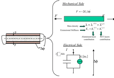
4-7 Mechanical and electrical equivalents of axially homogeneous PEM with in-phase connected PZT sheets . . . 62

4-8 Mechanical and electrical equivalents of axially homogeneous PEM with out-of-phase connected PZT sheets . . . 64

4-9 Bimorph PZT transducer on a elastic beam: lateral view . . . 71

4-10 Bimorph PZT transducer on a beam: cross section . . . 72

(9)

6-1 Basic Cell: Electric Connections . . . 105

6-2 Isolated Resonant Shunts (IRS ): Basic Cell . . . 111

6-3 Trasmission Line with Line Resistance and Inductance (TL-Rl-Ll): Basic Cell . . . . 111

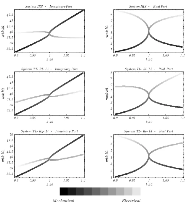
6-4 Trasmission Line with Line Inductance and Ground Resistance (TL-Rg-Ll): Basic Cell112 6-5 Real and imaginary parts of !(k); solution of the characteristic polynomial in the optimal system for trasverse-electric waves: comparison of network con…gurations . . 120

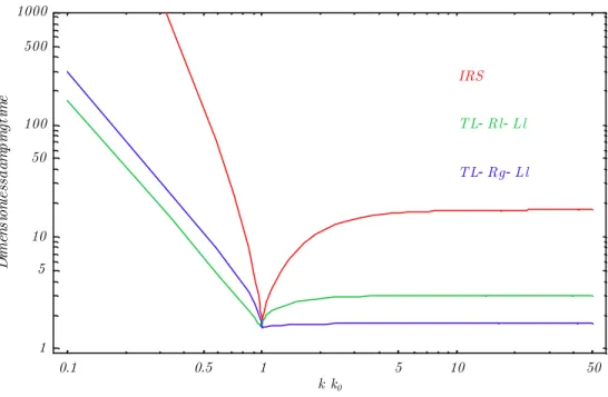
6-6 Dimensionless damping time as function of k=k0 . . . 121

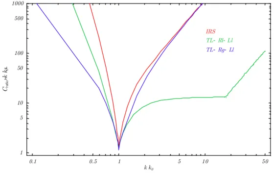
6-7 Ratio between the actual damping time and that one achievable in optimal conditions as a function of k=k0 . . . 122

6-8 Modal mechanical energies as a fuction of time for a simply supported PEM beam with di¤erent network topologies optimized for the …rst bending mode. . . 123

6-9 Dimensionless damping time as a function of k=k0 in systems that have been opti-mized for a wavenumber k0 . . . 129

6-10 Ratio between the actual damping time and that one achievable in optimal conditions as a function of k=k0 . . . 130

7-1 Pinned-pinned beam with …ve bimorph PZT pairs . . . 133

7-2 Realized beam with PZT transducers . . . 133

7-3 Single sheet piezoelectric transducer . . . 134

7-4 Characteristics of used PZT material. . . 134

7-5 PZT pair in bimorph con…guration: detailed constructive scheme. . . 135

7-6 Synthetic inductor: an alternative modi…cation of Antoniou’s GIC . . . 136

7-7 Synthetic Inductor: ideal equivalent impedance . . . 136

7-8 Synthetic Inductor . . . 137

7-9 RLC resonant circuit for experimental testing of the Antoniou’s GIC by frequency response measurements. . . 137

7-10 Batteries for alimentation of Op-Amps . . . 138

7-11 Acquisition and generation boards technical datasheets. . . 139

7-12 Logical scheme for Frequency Response measurements . . . 141

7-13 Experimental set up for mechanical FRF measurements . . . 142

7-14 Experimental set up for electrical FRF measurements . . . 143

7-15 Identi…cation procedure . . . 144

7-16 Results of the identi…cation of the …rst three modes of the simply supported alu-minum beam . . . 146

(10)

7-17 Statistical analysis on a set of 15 measures of the beam FRF: mean values and

uncertainties . . . 146

7-18 Synthetic inductor: experimental and theoretical equivalent inductance L vs resis-tance R6 . . . 147

7-19 E¤ect of R0 on the parasite resistance for a …xed equivalent inductance L = 210 H : . 147 7-20 Con…guration for the resonant shunted PZT experiment . . . 148

7-21 Frequency responce reduction for tuned resonant shunted PZT . . . 149

7-22 Poles of the coupled system varying the electric parameters . . . 149

C-1 Elementary cell of the electromechanical beam: lateral view. . . 157

(11)

List of Tables

6.1 Transverse-Electric waves: optimal values and sensitivities with respect to the wave

number of the electric parameters for di¤erent network con…gurations . . . 116

6.2 Transverse-Electric waves: optimal values of the electric dimensionless parameters for di¤erent network con…gurations . . . 117

6.3 Longitudinal-Electric waves: optimal values and sensitivities respect to the wave number of the electric parameters for di¤erent network con…gurations . . . 127

6.4 Longitudinal-Electric waves: optimal values of the electric dimensionless parameters for di¤erent network con…gurations . . . 128

A.1 Piezoelastic variables and characteristics: physical dimensions . . . 152

B.1 External actions: expressions and physical dimensions . . . 155

B.2 Material characteristics: expressions and physical dimensions . . . 156

C.1 Material characteristics:Expression and Numerical Values . . . 159

(12)

Chapter 1 Introduction

1.1 Background and Motivations

The control of structural vibrations is one of the foremost issues of mechanical engineering. Vi-brations are undesirable for reliability, comfort and functionality of mechanical devices. Indeed, they are a cause of material failure by fatigue, they generate noise that is disturbing for humans, they impose a limit to the achievable precision in machinery, their oscillations cause instability in aerodynamical systems, as happens for the wings of an airplane.

Traditional solutions to the problem are to utilize viscoelastic material to add damping to the structure or to design the mass and sti¤ness distribution to control its dynamical behavior. An alternative device for narrow band vibration damping is the Dynamical Vibration Absorber (DV A): It consists of a spring-mass-damper to be coupled to the system to obtain a resonant energy exchange and dissipation.

In the last decade many research e¤orts were devoted to study the applications to this …eld of the signi…cant electromechanical coupling o¤ered by the new generation of piezoelectric ceramics such as lead zirconate titanium (P ZT ). In this context active and passive techniques have been developed. Active controls use PZT materials as sensor and actuators to apply feedback control to the structure. These achieve good performances, but they present the disadvantages of an high power requirement, stability problems, and the need of a complex central unity for the implemen-tation of the control law. Passive solutions suggest to utilize the two way piezoelectromechanical coupling to transfer mechanical energy in electrical form and dissipate it in resistances by the Joule e¤ect. It has been show that resonant systems are more e¤ective to this aim. In analogy to DV As; piezoelectric transducers shunted on an inductance and a resistance can be bonded to a structure

(13)

to form a coupled highly dissipative system. Adjusting the electrical parameters, the RLC circuit1 can be tuned on a given mechanical mode with replacing it with a pair of strongly damped elec-tromechanical modes. The advantages of this solution are its constructive simplicity, its intrinsic stability and the total independence from the environment. Indeed, in principle passive devices not only do not require power to work, but they can even be used to produce small amounts of energy2. In practice the high inductor required to tune the mechanical system to the electric one are frequently synthesized with electronic circuit that require a small amount of power to work3_. Resonant Shunted Piezoelectrics (RSP) are strongly preferable to the mechanical analog DV As because of their low cost, low weight, low space requirements and for their ‡exibility. Indeed, the electrical parameters can be easily adjusted to match the characteristics of the structural mode to be damped. Exploiting this aspect, semi-active systems in which the values of the electrical param-eters are chosen by a real-time control unit have been proposed. Industrial applications of RSPs are now available (see for example www:acx:com where smart skis and smart bikes are illustrated). The greatest disadvantage of these devices are that they are e¤ective only in a narrow band of frequencies because of their one-degree-of-freedom resonant nature. To bypass this problem piezo-electric patches with multiple shunts, each one of which can be matched on a mechanical mode, have been proposed with good results.

An innovative idea presented by dell’Isola and Vidoli consists in establishing a distributed piezoelectric coupling between continuous mechanical and electric media to form a ”smart struc-ture”4 _{capable to be adjusted for an optimal broadband damping. They proposed to think about} controlling a continuous mechanical structure with its electrical analog to enhance a complete com-munication between the two systems. In the present work this idea is studied and implemented.

1.2 Literature Review

Hagood and Von Flotow [30] in 1991 presented the …rst complete analytical and experimental study on resonant and resistive shunted PZT s; proposing an optimization procedure analog to those adopted for Dynamic Vibrations Absorbers in classical texts on vibrations such as Timoshenko [10]. The subject has been developed also by Del Vescovo in [28], [29] presenting comparisons between

1_{The capacitance is given by the physical nature of P ZT materials, that are dielectrics.} 2_{Energy harvesting by PZT transducers is one of the most recent reaserch topics.}

3_{Let us underline that this power consumption is related only to the particular actual realization of a passive} device.

4_{Let us recall one of the most pertinent de…nitions of ”smart structure”:}

A smart structure is a material systems with intelligence and life features integrated in the microstructure of the material system to reduce mass and energy and produce adaptive functionality.

(14)

experimental results and numerical prediction. Details about the optimal design are given in [32] and in [33] by Ste¤en and Inman, both for active and passive control techniques. They propose also the simultaneous use of DV As and RSP s. Multiple shunts are implemented by Hollkamp [39]. Lesieutre [31] presented an useful review on shunting circuits (inductive capacitive, resonant and switched) giving design indications for applications. Active controls using piezoelectric materials as sensors and actuators are proposed in [40] and [41], semi-active techniques in [42] and [43].

Models of piezoelectric materials as actuators in unidimensional structures have been developed by Crawley in [35] and [36]. On the other hand their behavior as sensor has been investigated by Shiroy and Chopra in [37]. A coupled PiezoElectroMechanical model is discussed in [34], where also a Finite Element implementation is presented. Emphasis on experimental testing is given in [38].

Dell’Isola and Vidoli proposed a distributed coupling between mechanical and electrical continua to dissipate mechanical energy in the electrical form. In [20] they present a continuum model of a piezoelectromechanical truss beam coupled with an electrical transmission line studying its application for the suppression of longitudinal and torsional vibrations while in [21] they look for solutions for the bending modes. The idea of the distributed passive control is then applied in [22] to study, by means of an homogenized model, the modal coupling between a beam and a second order electric transmission line.

1.3 Ideas and Research Objectives

The goal of the research project of which this work is an integrated part is to study and realize electromechanical systems for distributed passive control of vibrations in mechanical structures by piezoelectric transducers and electric networks, following and improving what has been done in [20], [21], [22]. In this context theoretical, numerical and experimental work is required.

The physical idea to be developed is to couple by means of PZT transducers a given mechanical continuum with an electric continuous medium possessing analogous characteristics, in order to realize an electromechanical energetic exchange for a wide range of frequencies. Indeed, if waves propagate in the same fashion in two media and if they have been tuned for a given wavelength, hence they are tuned for all. In this way one of the crucial issues of collocated passive control, the narrow band behavior, can be solved.

To implement this idea in engineering applications it is necessary to 1. …nd electrical analogs of mechanical systems

(15)

2. realize the coupling between the analogous electrical and mechanical systems In …nding the analog electrical continuum two di¢culties are encountered:

1. the speed of propagation of energy in electrical continua is enormously di¤erent to that in mechanical media

2. the physics of electromagnetism and mechanics are not the same. There can be physical mechanical phenomena that have not an electric equivalent and vice-versa.

For these reasons it is required to synthesize in an approximative fashion the electric media by a lumped model. Then the coupling between the mechanical continuum and the electric lumped periodic system can be achieved by means of an array of piezoelectric transducers. With this idea we will focus our attention on periodic electromechanical systems similar to that whose basic cell is sketched in …gure 1-1. g R g L l R l L g R g L l R l L g R g L l R l L g R g L l R l L g R g L l R l L g R g L l R l L g R g L l R l L

Figure 1-1: Periodic piezoelectromechancial beam

While a parallel study on electrical analogs of mechanical systems is carried on, the present work has the following main objectives:

1. to establish both re…ned and homogenized models of the periodic electromechanical systems with distributed piezoelectric coupling. Modular dissipative piezoelectromechanical systems composed by a mechanical continuum connected to a lumped electric network by means of an array of PZT transducers will be considered. It will be necessary to develop

(a) a detailed model of the interaction between piezoelectric transducers and structures that underlines the two way electromechanical coupling, understanding how and by which hypotheses it can be simpli…ed,

(16)

(b) develop a re…ned model of the modular piezoelectromechanical system,

(c) develop following [20], [22] homogenized models, identifying the constitutive relations by those found for the re…ned ones.

2. to study and compare the qualitative features of di¤erent types of electric networks for the suppressions of mechanical extensional and ‡exural vibrations. In particular, considering modular piezoelectromechanical media, we want to

(a) optimize the value of the electric parameters in the networks for a series of di¤erent topologies to maximize the vibration damping,

(b) perform a scale analysis, understanding the in‡uence of the ratio between the length of the basic module and the characteristic wave lengths on the value of the optimal electric parameters and in the performances of the system for the vibration damping,

(c) understand why and how optimized electrical systems with di¤erent topologies have di¤erent performances to damp mechanical vibrations.

3. to realize and study experimentally the proposed piezoelectromechanical systems. It will be necessary to

(a) realize prototypes, facing the related technological problems

(b) design and test an experimental set up and measurement procedure for their testing (c) verify experimentally the analytical and numerical results.

Constructive critical feedback between the experimental and modelling aspects will be crucial in this work. Indeed, in the research project the present is the …rst step toward an experimental realization of the proposed devices.

1.4 Outline

The present paper can be structured in three main parts. In each of them one of the three main objectives that have been outlined in the previous section will be treated.

In the …rst part composed by chapter 3,4,5 models of piezoelectromechanical systems will be developed. In particular, in chapter 3 the attention will be focused on electric systems presenting and modelling the electric networks that will be utilized for vibration damping. Some words on electromechanical analogies will be spent. In chapter 4 a re…ned unidimensional model of an elastic

(17)

beam on which PZT patches are bonded will be given. The system will be considered as a multi-layer beam and its model will be deduced by the three-dimensional one imposing a given mechanical and electrical kinematics. The equations of motion will be furnished both in the strong and weak form, having mind future studies involving the determination of numerical solutions also for the re…ned model of the proposed smart structures. The hypotheses and the con…gurations for which the interactions between elastic and piezoelectric layers can be reduced to a simple model will be underlined. In chapter 5 the results achieved in chapter 3 and 4 will be applied to assemble the re…ned model of a periodic unidimensional piezoelectromechanical medium composed by an elastic beam coupled by means of a distributed array of PZT transducers to a lumped electric network. A continuous model of the periodic system will be derived by means of an homogenization procedure. Both the cases in which the electrical variables are coupled to the mechanical extensional and ‡exural behavior will be studied.

In the second part (chapter 6), the homogenized model previously deduced will be utilized to optimize the electrical networks for the vibration suppression and to infer important thumbnail informations about the characteristics of the system. A wave approach will be followed to perform a comparative analysis between di¤erent network connections. We will study the dependence of the optimal electric parameters on the dimensions of the basic cell of the periodic system, their sensitivity with respect to a change in the considered wavelength and the performance of the optimal systems for vibration damping.

In the third part (chapter 7) the problem of the experimental realization and testing of the pro-posed piezoelectromechanical system for the suppression of mechanical vibration will be addressed. The realized experimental apparatus and a tested measurement procedures will be described. The results of a classical experience on shunted PZT s; that has been reproduced to validate the exper-imental setup, will be presented. Finally future experiments will be designed.

In the following chapter the basic concept of continuum mechanics and piezoelectricity will be recalled. Moreover, referring to [3], the notation and the basic features of the Virtual Power Principle, whose modelling approach is adopted, will be presented.

(18)

Chapter 2 Preliminaries

In this chapter the basic concept of the kinematics of a continuum body will be recalled. Some words will be spent on the meaning and the formalism of the Virtual Power Principle that will be largely used in this work to derive the balance equations of dissipative electromechanical discrete and continuous systems. Finally the constitutive behavior of a piezoelectric material will be discussed furnishing applicative examples.

2.1 Continuum Kinematics

2.1.1 Body, References, Coordinates

A body can be identi…ed with the closed region of the Euclidean spaceE that it occupies at a given instant in time. We will call this region the reference con…guration_{B and the points p 2B material} points. Once a …xed Cartesian reference frame C = fo; e1; e2; e3g is selected each point p can be associated with the oriented arrow ¡op:! Thus the space of points p can be structured as vector space V and each point can be represented also by the coordinate representation of ¡!op in_C:

1

e

2

e

3

e

O

E

1

p

3

p

2

p

Reference frame

(19)

We will denote by

e=_fe1; e2; e3g (2.1)

the …xed basis for _{V and by}

p=¡op!= p1e1+ p2e2+ p3e3 = epe= e 2 6 6 6 4 p1 p2 p2 3 7 7 7 5 (2.2)

the vector p =¡op! with coordinates pe in the e basis.

We will introduce in _{V a scalar product " ¢ " that is a bilinear, symmetric, positive de…nite} application between pairs of elements of_{V. If not otherwise speci…ed, the scalar product is de…ned} such that e_{¢ e :=} 2 6 6 6 4 e1¢ e1 e1¢ e2 e1¢ e3 e2¢ e1 e2¢ e2 e2¢ e3 e₃_{¢ e}₁ e₃_{¢ e}₂ e₃_{¢ e}₃ 3 7 7 7 5= I (2.3)

where I is the third order identity matrix.

2.1.2 Deformations of Continuum Bodies

De…nition 1 A deformation of a body B is a mapping

f : B 7! E

f : p7! x := f(p)

For the physical requirement of the impenetrability of the bodies and its continuity, f(p) must be a smooth 1-1 mapping from _{B to a bounded region of E: An important role in the description} of a deformation of a continuum body is played by the deformation gradient with respect to p

(20)

whose determinant represents the local change in volume under f: We must require det(rf (p))6=0 for each p_{2 B: We will assume}

det(rf (p)) >0; f or each p_{2 B:} (2.5)

De…nition 2 Let _{V be the three dimensional vector space of translations of B. The displacement} …eld associated to the deformation f is a function

^

u : _{B 7! V} ^

u : p7! u = ^u(p) := f(p)¡ p Remark 1 The displacement gradient respect to p is

ru = r(f(p) ¡ p) = F ¡ I

F;_{ru are linear applications from V to V we say F;ru 2 Lin(V ). In particular F 2 Lin}+₍_V) De…nition 3 A deformation f is called an homogeneous deformation if F(p) is constant for each p_{2 B}

Let us introduce in the vector space of oriented arrows the norm_{k¢k induced by the ordinary} scalar product. Thus it is possible to de…ne the distance between two points p; q by means of k¡!pq_{k = kp ¡ qk :}

De…nition 4 A deformation f is a rigid deformation if it preserves distances between any pair of points of the body B.

It is possible to show that the deformation gradient of a rigid deformation is skew-symmetric. Expanding a generic deformation in the neighborhood of a point q2 B we can approximate its behavior as the superposition of a translation and an homogenous deformation

f(p) = f (q) + F(q)(p_{¡ q)+o(p ¡ q)} (2.6)

The deformation gradient F can be decomposed in its symmetric part E and skew symmetric part W as following

(21)

where D = 1 2 ¡ F+ FT¢ (2.8) W = 1 2 ¡ F_{¡ F}T¢ (2.9)

In the same way the displacement gradient_{ru can be decomposed as}

ru = S + W (2.10) where S = 1 2 ¡ ru+ruT¢ _(2.11) W = 1 2 ¡ ru¡ruT¢ (2.12)

and S is called the in…nitesimal strain

Thus each deformation can be locally decomposed in a rigid deformation and in a pure defor-mation as

f(p) = f(q) + D(q)(p_{¡ q) + W(q)(p ¡ q)+o(p ¡ q)} (2.13) where

f(q) + W(q)(p_{¡ q)} (2.14)

is the rigid component of f and

D(q)(p¡ q) (2.15)

is the pure deformation. We denoted by o(p¡ q) higher order terms in the Taylor expansion of f(p) in a neighborhood of the point q

If dynamical processes are considered, an appropriate terminology must be introduced.

(22)

for t in a given real interval I. It can be represented by the function x : _{B £ I ! E}

: (p;t)! x =x(p;t) := ft(p)

De…nition 6 The velocity …eld v(p;t) for a given motion x(p;t) is de…ned as v(p;t) :=@

@tx(p;t) =:_x(p;t)

Obviously the time derivatives of all the …elds previously introduced can be de…ned.

De…nition 7 Let p and q be points of the euclidean space E. A velocity …eld v(p;t) is a distributor if

v(p;t) = v(q) + - (t)(p_{¡ q)} where - (t) is a skew-symmetric linear transformation.

The velocity …eld v(x;t) is one of a motion described by

x= Q(t)(p¡ o) + c(t) (2.16)

with

Q(t)QT(t) = I (2.17)

and

- (t) = _Q(t)QT(t) (2.18)

De…nition 8 A tensor valued …eld in _R3 _{is said to be objective if and only if its components} transform tensorially with respect to (2.16).

Let_{C be the linear space of the distributors C.}

Remark 2 Since each C _{2 C is the superposition of a translation and a rotation in the euclidean} space E, the dimension of C is 6:

(23)

De…nition 9 A motion belonging toC is said to be rigidifying motion if B is a deformable contin-uum.

2.1.3 Beam Kinematics

Let us consider in the Euclidean spaceE a straight line A; called axis, a point O on it, called origin and a one parameter family of bounded plane regions_Sx; x 2 I ½ R, called sections. It is now possible to …x a Cartesian reference frame C = fO; e1; e₂; e₃g, with origin O and the e1 ¡ axis parallel to_A.

A straight axis beam_{B can be geometrically described as the union of sections S}x for x in some closed interval I of R. Formally

B := [ x2I

Sx (2.19)

The oriented arrow ¡!OP that is an element of the vector space _{V of translations in E, can be} associated at each point p_{2 B. In the reference C}

¡!

OP = p1e1+p2e2+p3e3 (2.20)

and the set of three real numbers fp1; p2; p3g is the coordinate representation of¡!OP inC. ¡!OP can be partitioned in its orthogonal projection on the axis _A

¡¡!

OPa= p1e1 (2.21)

and its orthogonal projection on the section _Sx

s:= ¡¡!PaP = p2e2+p3e3 (2.22)

such that

¡!

OP = ¡¡!OPa+ ¡¡!PaP (2.23)

where ¡¡!OPa is an element of the three dimensional vector space V and s := ¡¡!PaP lies in the two dimensional vectorial space _{W of the translations in the plane.}

(24)

de-scribed by the smooth one parameter family of smooth maps

x(_{¢ ;t) : B 7! B}t (2.24)

such that each point p in the reference con…guration _{B is mapped into its position q in the actual} con…guration_Bt at time t by

¹

x= x(p;t) (2.25)

The displacement vector …eld is naturally de…ned as follows

u(p;t) = ¹x_{¡ p = x(p;t) ¡ p} (2.26)

Remark 3 In the basis e =_fe1; e2; e3g u(pa; t) can be written as

u(p;t) =u1(p1; p2; p3; t)e1+ u2(p1; p2; p3; t)e2+ u3(p1; p2; p3; t)e3 We will use the following notation

u(p;t) =e (u(p;t))e = e 2 6 6 6 4 u1(p1; p2; p3; t) u2(p1; p2; p3; t) u3(p1; p2; p3; t) 3 7 7 7 5

where e is the row vectorfe1; e2; e3g and the column vector (u(p;t))e is the coordinate representation of u(p;t) in the basis e: In the same fashion

x(p;t) =e (x(p;t))_e = e 2 6 6 6 4 f1(p1; p2; p3; t) f2(p1; p2; p3; t) f3(p1; p2; p3; t) 3 7 7 7 5

Moreover, given a function g(p1; p2; p3; t); we will de…ne g(p1; t) := g(p1;0; 0; t)

The partition of ¡!OP induces the de…nition of the one parameter family of applications

(25)

such that x(p;t) = x(pa; t) + Gt(s): (2.28) where pa= ¡¡!OPa= e 2 6 6 6 4 p1 0 0 3 7 7 7 5; s= p¡ pa (2.29)

The constraints imposed on Gt play a fundamental role in beam modelling. We will assume that the axis can move only in the e2; e3¡ plane and that Gt is the composition of a in plane uniform deformation Utand a rotation Rt around the e2¡ axis: Thus

Gt(v) = Rt(Ut(v)) (2.30)

where U :_{W 7! W is linear and R}t:W 7! V has the following coordinate representation in the basis e =fe1; e2; e3g for V and e0=fe2; e3g for W

(Rt)e 0 e = 2 6 6 6 4 0 sin(µ) 1 0 0 cos(µ) 3 7 7 7 5 (2.31)

De…nition 10 A beam has no shear deformation if the rotation Rt of the section Sx is such that in the actual con…guration the angles between the sections and the axis remain the same those in the reference con…guration.

We will linearize the kinematics about the reference con…guration and we will assume that the beam has no shear deformability.

Claim 1 In the linearized kinematics the rotation Rt has the following coordinate representation in the e¡ e0 ¡bases (Rt)e 0 e = 2 6 6 6 4 0 µ 1 0 0 1 3 7 7 7 5

(26)

Rt is

µ=_¡@x3(p1; t) @p1 =¡

@u3(p1; t) @p1

Finally we can write the coordinate representation of the motion beam without shear deforma-tion in the linear approximadeforma-tion

(x(p;t))_e = 2 6 6 6 4 x1(p1; t) 0 x3(p1; t) 3 7 7 7 5+ 2 6 6 6 4 0 _¡@x3(p1;t) @p1 1 0 0 1 3 7 7 7 5 2 4 U11 U12 U21 U22 3 5 2 4 p2 p3 3 5 = 2 6 6 6 4 x1(p1; t)¡@x3@p(p₁1;t)(p2U21+ p3U22) p2U11+ p3U12 x3(p1; t) + p2U21+ p3U22 3 7 7 7 5

Remark 4 In the hypotheses of rigid sections U = I and

x(p;t) = e 2 6 6 6 4 x1(p1; t)¡ @x3_@p(p₁1;t)p3 p2 x3(p1; t) + p3 3 7 7 7 5 (2.32) u(p;t) = e 2 6 6 6 4 u1(p1; t)¡ @u3_@p(p₁1;t)p3 0 u3(p1; t) 3 7 7 7 5 (2.33)

2.2 Virtual Power Principle

2.2.1 Introduction

Our goal is to deduce homogenized and re…ned models of electromechanical dissipative systems. The variational principle of virtual power, that is an evolution of D’Alembert principle, leads us to a weak formulation of the problem that is general enough to consider the electromechanical coupling in dissipative processes. In this context the equilibrium is expressed by a balance of powers. The basic idea of this formulation is to describe forces not by their vectorial representation but by means of the power they exert for a given velocity …eld1. In other words once given the normed vector spaceV of virtual velocity …elds v; the forces f acting on them are determined by the scalar values

(27)

assumed by the linear functional

P : V ! R

: v! P(v) = hf; vi

In this way the duality via a bilinear form_{h¢; ¢i between the linear vector space of forces and virtual} velocities is the way in which the forces are de…ned.

2.2.2 De…nitions

State variables

Discrete and continuous systems are distinguished by the fact that at a given instant in time the con…guration of a discrete system is given by a set of k constants

X=_fx1; :::; xkg (2.34)

while the con…guration of a continuum body2 _{B is given by a set of h …elds de…ned on B}

U0=fu1(p); :::; uh(p)g (2.35)

and eventually by their spatial gradients

U1; :::; Un where

Ui =friu1(p); :::;rium(p)g; m · h; i = 1:::n (2.36) The local state of a continuum body in the neighborhood of each point must be speci…ed explicitly and its description will be as good as the greatest gradient order n considered (the concept of a Taylor expansion of each …eld ui(p) should be kept in mind). The choice about which and how many spatial gradients to consider is a constitutive assumption. A theory which considers n spatial gradients is called n_{¡ th gradient order theory.}

On a continuum body a set of boundary conditions must be prescribed. In the approach we 2_{Here as before a continuum body is identi…ed with the region B of the Euclidean space that it occupies at a …xed} time instant t0

(28)

are following only the boundary conditions prescribed directly on the elements of U = U0; :::; Un (essential boundary conditions) must be explicitly considered. They will be in the form of nbc equations (BC), in general non-homogeneous, that must be satis…ed on a part of @B and they appear in the de…nition of the functional space in which the virtual velocities must lie.

We will focus our attention on a system_{S constituted by a continuum body B with a set of} essential boundary conditions BC: The state ofS at a …xed instant in time is given by the set

S=fU0; :::; Ung: (2.37)

We will call S the set of the state variables of _S:

Example 1 In a …rst order gradient theory the state of an electromechanical continuum in the quasi-electrostatic approximation can be described by

S =fu(p; t); Á(p; t); ru(p; t); rÁ(p; t)g; p 2B (2.38) where u(p; t) is the vectorial valued …eld describing the mechanical displacement from the reference con…guration and Á(p; t) is the scalar valued …eld of the time primitive of the electric potential. Actual and Virtual velocities

The elements of S are all functions of time and the set of their time derivatives

V =fV0; :::; Vng (2.39)

where

Vi =friu_1(p); :::;riu_m(p)g; m · h; i = 1:::n (2.40) are a velocity description of _{S: Here we will distinguish between the velocity actually experienced} during a motion (actual velocities) and the virtual velocities that will be denoted by a superscript "¤". The virtual velocities do not need to satisfy the equation of motions, they are required only to be enough smooth and to satisfy the homogeneous version of the prescribed boundary conditions, otherwise they are arbitrary. We will denote byV the vector space of the virtual velocities.

On the actual and virtual velocities the same smoothness is required, but in general the func-tional spaces in which they lie are di¤erent because of the boundary conditions. In fact the actual velocities _ui(p) must satisfy the prescribed essential boundary conditions while the virtual

(29)

veloci-ties are required to satisfy their homogeneous version. For numerical application it is useful to have the actual and virtual velocities in the same space. Thus if non-homogenous boundary conditions are present it is convenient to restate the problem converting them to an homogeneous form3.

Focusing our attention on a …rst gradient order theory, let us denote the vector space of virtual velocities by

V = fv¤i;rv ¤

igi=1:::n=f_si;r_sigi=1:::n (2.41)

The virtual velocities that are objective are called objective virtual velocities. Let’s denote by Vobj the space spanned by them:

Example 2 In an electromechanical continuum in the quasi-electrostatic approximation and for a …rst order-gradient theory the following set of virtual velocities can be chosen

V = f _u¤(p;t); Á¤(p;t);_{r_u}¤(p;t);_{r_Á}¤(p;t)_g (2.42) Virtual Powers

The virtual powers are de…ned as a linear functional de…ned on the space_{V of the virtual velocities.}

P : V ! R (2.43)

Thus the virtual powers are in the dual space of_{V: The virtual velocities are test functions for the} forces de…ned in the distributional sense by means of the corresponding powers.

Virtual Power of Internal Forces The virtual power of internal forces is characterized by the following

Axiom 1 The virtual power of forces internal to a system _{B vanishes for all rigidifying motions} of B considered at any time t.

Proposition 1 The virtual power _Pintof the internal forces © exerted within a continuous medium that occupies, in the reference con…guration, the region _{B of the euclidean space is expressed by a}

(30)

continuous linear functional on the normed4 linear space Vobj:That is Pint(B; V) = h©; v¤iB; v

¤

2 Vobj:

Thus to formulate an a-priori theory of a continuum it is necessary, after having chosen the space _{V; to …nd V}obj:In the present work we will specialize already existence theories in technical cases and we will write directly the expression of the internal power without facing the problem of …nding_Vobj.

Example 3 In an electromechanical continuum in the quasi-electrostatic approximation and for a …rst order-gradient theory the virtual velocity are (2.42) and

Vobj=f _S¤(p;t);r _Á ¤ (p;t)_g (2.44) where _ S¤(p;t) = sym(_{r _u}¤(p;t)) =1 2(r_u ¤ (p;t)+_{r_u}¤(p;t)) (2.45)

Hence the virtual power of the internal forces is

Pint(B; V) = Pint;m(B; V ) + Pint;e(B; V) (2.46) = DT; _S¤(p;t)E

B+ D

J;r _Á¤(p;t)E

B (2.47)

where the tensorial …eld T and the vectorial …eld J are de…ned as the quantities on which _S¤_; r_Á¤ expend power. Physically T is the tensor that describes the tensional state of a continuum, while J can be interpreted as the time derivative of the electric displacement vector D, that is a displacement current inside the dielectric body.

Virtual Power of External Forces As the external forces are classi…ed as at-distance, or volume, forces and contact forces, so are the respective powers.

Proposition 2 The virtual power of distance, or volume, forces Bdexerted in a continuous medium occupying, in the reference con…guration, the region _{B of the euclidean space E, is a continuous}

4_{The norm induced by the scalar product h¢; ¢i}

(31)

linear functional onV.

Pd(B; V) = h©; v¤iB := Z

B

Bd¢ v¤

Proposition 3 The virtual power of contact forces Bcexerted in a continuous medium occupying, in the reference con…guration, the region_{B of the euclidean space E, is a continuous linear functional} on V.

Pc(@B; V ) = h©; v¤i@B := Z

@B

Bc¢ v¤

The external forces can expend power in every type of virtual velocities, included the non objective ones. Often in applications only a few types of them are present.

Here we will considered the inertial forces as external forces despite that they are prescribed by something similar to a constitutive relation, while contact and volume forces are given by the environment in which the body is embedded.

Proposition 4 The virtual power of inertial forces _Pa experienced by a continuous medium occu-pying the domain _{B of the euclidean space E in the reference con…guration is a continuous linear} functional on the virtual velocities containing only time derivatives of the state …elds and not their gradients.

For example, in the purely mechanical case we will impose Pa(B; v¤) =

Z

B¡½ _v ¢ v ¤

(2.48) where ½ is the mass density for unit volume in the medium. We underline that it is necessary to di¤erentiate the notation between the actual velocities v and the virtual velocities v¤: The minus sign in the de…nition is due to the fact that they are considered as external forces.

The virtual power of all the external forces is given by the sum of the three contributions Pext(B; v¤) =Pd(B; v¤) +Pc(@B; v¤) +Pa(B; v¤) (2.49) Example 4 Let_{B be an electromechanical dielectric in the quasi-electrostatic approximation. The} virtual velocities are (2.42) and the virtual power of the external forces can be written as

(32)

Power of distance forces

Pd(B; v¤) = Pd;m(B; _u¤(p;t)) (2.50) = hb; _u¤

(p;t)iB (2.51)

Power of contact forces

Pc(@B; v¤) = Pc;m(@B; _u¤(p;t)) +Pc;e(@B; _Á ¤ (p;t)) (2.52) = _{hf; _u}¤(p;t)_i@B+ D ¾; _Á¤(p;t)E @B (2.53)

Power of inertial forces

Pa(@B; v¤) = Pa;m(@B; _u¤(p;t)) (2.54)

= _{h¡½Äu(p;t); _u}¤(p;t)_iB (2.55)

Hence the total power of the external forces is

Pext(B; v¤) = Pd(B; v¤) +Pc(@B; v¤) +Pa(B; v¤) (2.56) = 0 @ Pd;m(B; _u ¤_{(p;t)) +} Pc;m(@B; _u¤(p;t))+ +_Pc;e(@B; _Á ¤ (p;t)) +_Pa;m(@B; _u¤(p;t)) 1 A = 0 @ R Bb¢ _u ¤_{(p;t) +}R @Bf ¢ _u ¤_(p;t)+ +R_@B¾ _Á¤(p;t) +RB¡½Äu(p;t)¢ _u ¤ (p;t) 1 A

2.2.3 Statement

It’s …nally possible to enunciate the principle of virtual power.

Proposition 5 Principle of Virtual Power. In a Galilean reference frame, and for an absolute Newtonian chronology, the virtual power of the internal forces of a system _{B balance the virtual} power of external forces impressed on the system, for any smooth virtual velocity …eld satisfying the homogeneous version of the prescribed boundary conditions. Thus the following equality must hold for each smooth v¤ _{satisfying the homogeneous version of the prescribed boundary conditions}

Pint(B; v¤) =Pext(B; v¤) (2.57)

(33)

…rst order gradient theory the virtual velocities are (2.42), the virtual power of the internal forces is (2.46), the virtual power of the external forces is (2.56). Hence the power balance is expressed by

Pint;m+Pint;e = Pd;m+Pc;m+Pc;e+Pa;m (2.58)

0 @ R BT¢ _S ¤_(p;t)+ +R_BJ_{¢ r _Á}¤(p;t) 1 A = 0 @ R Bb¢ _u ¤_{(p;t) +}R @B¾ _Á ¤ (p;t)+ +R_@Bf_{¢ _u}¤(p;t) +R_B_{¡½Äu(p;t) ¢ _u}¤(p;t) 1 A

2.2.4 Considerations

From a kinematical description of the physical system by means of the principle of the virtual power, once considered the constitutive equations, a mathematical formulation of a boundary value problem can be obtained.

The formulation of a physical problem by means of the principle of the virtual power allows us to

1. Obtain a weak formulation of the problem. It is given by the statement of the principle power itself when the constitutive relations are considered.

2. Derive a Galerkin Formulation of the problem restating the principle of the virtual power performing a change of variables in order to have only essentially homogeneous boundary conditions.

3. Obtain numerical approximate solutions for the problem by means of a Galerkin Approxima-tion. For example the Finite Element Method can be applied.

4. Derive the strong form of the balance equations rewriting the power balance with some inte-gration by parts and considering that the virtual velocities are arbitrary: It must be underlined that, dealing with non-regular physical systems, a strong formulation of the equilibrium equa-tions is not convenient because, while an analytical solution cannot be achieved, a numerical solution of the problem can be obtained directly as in 3.

5. Write the actual power balance for the system once the virtual velocities in (2.57) are substi-tuted by the actual velocities:

6. Find a correspondence between the forces appparing in two di¤erent models of the same phys-ical system once a kinematphys-ical map between them is given. It can be obtained imposing that corresponding forces expend the same power in corresponding virtual velocities. With this procedure constitutive equations of homogenized models of periodic systems can be evaluated from re…ned models. The latter possibility is central in this work.

(34)

2.3 Piezoelectric Materials

In a piezoelectric material mechanical phenomena are coupled with electrical ones by means of constitutive relations. Here we will recall the constitutive equations of Linear Piezoelectricity.

2.3.1 Linear Constitutive Relations

The state of a piezoelectric material is no longer determined only by the mechanical state variable. Electromechanical interactions are not negligible and it is necessary to introduce new …elds to describe the electric state. We will consider the quasi-electrostatic case in which coupling between electrostatic and magnetic …elds can be ignored and only the electrostatic state is included in the model. Di¤erent choices of the electrical state variable are possible (electric displacement vector D, electric …eld vector E, electric potential Á, ...).

The coupling between the electrical and mechanics …elds is realized by means of the constitutive relations. The constitutive laws can be derived from a postulated expression of the Gibbs free energy and their explicit formulation depends upon the chosen mechanical and electrical state variables (see [7]). In the following we express the vectorial and tensorial quantities in a …xed orthonormal referenceC =f0;eg with the indicial notation (repeated indices are intended to be summed). Claim 3 The Gibbs free energy for a piezoelastic body is the scalar function

G=_¡TijSij¡ DhEh

where the electric …eld vector Eh and the mechanical strain tensor Sij are intensive state variables and the electric displacement vector and the mechanical stress tensor are extensive state variables. Depending upon which state variables are chosen as independent the following four equivalent expressions of the constitutive relations can be derived5:

² (S; D)-type (extensive type)

Tij= cD_ijklSkl¡hijnDn Em=¡hmijSij+¯SmnDn

(2.59)

(35)

where cD ijkl= h @G @Sij@Skl i D hijn = h @G @Skl@Dn i ¯Smn= h @G @Dm@Dn i S (2.60)

² (T; E)-type (intensive type)

Sij = sEijklTkl+ dijnEn Dm= dmijTij+ ²TmnEn (2.61) where sE ijkl= h @G @Tij@Tkl i E dijn= h @G @Tkl@En i ²S mn= h @G @Em@En i S (2.62)

² (T; D)-type (mixed type)

Sij = sD_ijklTkl+ gij mDm Em=¡gij mTij+ ¯TmnDn (2.63) where sD ijkl = h @G @Tij@Tkl i D gij n= h @G @Tkl@Dn i ¯Tmn= h @G @Dm@Dn i S (2.64)

² (S; E)-type (mixed type)

Tij= cEijklSkl¡eijmEm Dm=eijmSij+²SmnEn (2.65) where cE_ijkl=h_@S_ij@G_@S kl i E eij n= h @G @Skl@En i ²S mn= h @G @Em@En i S (2.66)

Remark 5 The state variables S; T; D; E can be replaced by other physical quantities. In these the constitutive relations can be rewritten considering the expressions of the new variable in term of the old ones.

(36)

Example 6 If the time primitive Á of the electric potential is chosen as state variable, the consti-tutive equations should be expressed in term of the pair of electric variables (Á; J). Since

Em= @ _Á @xm

; Jm= _Dm (2.67)

the (S; E)-type relations becomes

Tij = cE_ijklSkl¡eijm_@x@_m _Á Jm=eijmS_ij+²Smn@x@n

Ä Á

(2.68)

2.3.2 Voigt Notation

Piezoelectric materials present a particular symmetry: they are transversely isotropic with respect to an axis, called the polarization axis P. If a reference system is oriented according to that sym-metry, the parameters required to de…ne the coordinate representation of the constitutive relations are drastically reduced6. Moreover adopting a particular notation, valid only in the …xed reference, the material characteristics can be given in a matrix form.

Let us orient a reference C =_{fO; eg such that the e}3¡ axis will be parallel to the polarization direction P and let us denote with 1; 2; 3 the directions associated to e1; e2; e3. If the following correspondence between each pair of indices ij of the tensorial notation and a index r of the so de…ned Voigt-Kelvin notation is introduced

11_{! 1} 22_{! 2} 33_{! 3}

23 = 32_{! 4 13 = 31 ! 5 12 = 21 ! 6} (2.69)

the constitutive equations assume a simpler form and a matrix representation of them will be possible.

Remark 6 The experimental data for the constitutive behavior of the piezoelectric material are given in the Voigt notation and in particular in the intrinsic (S; D)-type or alternatively in the mixed (S; E)-type.

Example 7 The constitutive equations of the (S; E)¡ type for a linear piezoelastic material, ex-6_{Because of the transverse isotropy the piezoelectric constitutive equation must be invariant under the group of} rotations around the polarization axis.

(37)

pressed in the tensorial notation by (2.65), in the Voigt notation becomes S = sE_T _{+ dE}

D= dT + ²TE

(2.70)

where now S; T are 6x1 matrices, E; D 3x1 matrices and sE_{; d; ²}T _{are 6x6; 6x3; 3x3 matrices} ex-pressed by SE = 2 6 6 6 6 6 6 6 6 6 6 6 6 4 sE 11 sE12 sE13 0 0 0 sE₂₁ sE₂₂ sE₂₃ 0 0 0 sE 31 sE32 sE33 0 0 0 0 0 0 sE 44 0 0 0 0 0 0 sE 44 0 0 0 0 0 0 2(sE 11¡ sE12) 3 7 7 7 7 7 7 7 7 7 7 7 7 5 d = 2 6 6 6 6 6 6 6 6 6 6 6 6 4 0 0 d31 0 0 d31 0 0 d33 0 d15 0 d15 0 0 0 0 0 3 7 7 7 7 7 7 7 7 7 7 7 7 5 ; ²T = 2 6 6 6 4 ²T 11 0 0 0 ²T 22 0 0 0 ²T 33 3 7 7 7 5

The zeros entries in the matrices are due only to the symmetries.

2.3.3 Uniaxial States

Frequently particular physical situations allow to neglect the in‡uence of some secondary phenom-ena on the main aspects that one wants to model, consequently the number of variables needed to describe the state of the system can be reduced. Here we will give the de…nition of some of those situations and we will derive the corresponding constitutive equations, in order to use them in the following sections.

De…nition 11 A tensional state is called uniaxial along the i_{¡ axis if all the stress components} vanish except the one along the i_{¡ axis: Using the Voigt notation, a uniaxial tensional state in the} 1¡ direction is characterized by

(38)

De…nition 12 The electrostatic state is called uniaxial along the i¡ axis if all …eld components not parallel to the i_{¡ direction are zero. Using the Voigt notation,a uniaxial electrostatic state in} the 3¡ direction is characterized by

E1= E2 = 0; D1= D2= 0

In the following we will focus our attention on the piezoelectric material with a uniaxial ten-sional state along the 1_{¡ direction and a uniaxial electrostatic state along the 3 ¡ direction: We} characterize this situation as follows:

Claim 4 In a uniaxial stress state along the 1_{¡ direction and a uniaxial electrostatic state along} the 3_{¡ direction, equation (2.70) in the Voigt notation becomes}

2 4 S1 D3 3 5 = 2 4 s E 11 d31 d31 ²T33 3 5 2 4 T1 E3 3 5 (2.71)

Claim 5 In a uniaxial stress state along the 1¡ direction and a uniaxial electrostatic state along the 3_{¡ direction, equation (2.63) becomes}

2 4 S1 E3 3 5 = 2 4 s D 11 g31 ¡g31 ¯T33 3 5 2 4 T1 D3 3 5 (2.72)

In following sections we will often use the inverse of the (2.72) that is 2 4 T1 D3 3 5 = 2 4 c E 11 ¡e31 e31 ²S33 3 5 2 4 S1 E3 3 5 _(2.73) where cE11 = _s1E 11 ² S 33= ¡d2 31+²T33sE11 sE 11 e3₁= d31 sE 11 (2.74)

2.3.4 PZT Transducers

In this work we will refer to a piezoelectric transducer as a specimen of polarized PZT material whose surfaces are plated in order to generate a electric …eld inside the body once a potential di¤erence is applied between them. These conductive surfaces are called the electrodes. Depending upon the geometrical shape, the direction of polarization, and the direction along which the electric

(39)

…eld is applied, there are a great variety of PZT transducers able to couple the applied electric …eld with the mechanical shear or normal modes.

For applications to vibration control the most common con…guration is the one in …gure 2-1 where the transducer is constituted by a thin sheet of PZT material polarized along its thickness. Since the thickness tp is usually 10¡ 20 times smaller than the transversal dimensions this type of transducer can be treated as an essentially two dimensional object. When a voltage di¤erence is applied between the two electrodes an electric …eld is induced along the 3_{¡ direction and by the} relations (2.65) a constant mechanical pre-stress along the 1 and 2 directions is generated. If no forces are applied on the lateral surfaces the result of the applied …eld is a uniform contraction or elongation in the 1_{¡ 2 plane.}

p l p w p t Plated Surface Direction of Polarization V ∆ + -1 2 3

Figure 2-1: PZT sheet working by 3_{¡ 1 e¤ect}

When uniaxial stress states are considered the behavior of the PZT sheet is completely described by relations like (2.73). The manufacturers usually provide the performances of the PZT sheets giving the blocked force and the free elongation. These two quantities refer to a unidimensional model of the transducer. The blocked force is de…ned as the force exerted when the ends of the actuator are …xed and a given voltage is applied between the electrodes; the free elongation is the elongation experienced in the relevant direction for a given potential when no forces are applied. These characteristics can be derived also integrating equation (2.73) in order to get global constitutive relations of the type

2 4 F Q 3 5 = 2 4 kmm kme kem kee 3 5 2 4 ¢L V 3 5 (2.75)

where ¢L is the total elongation, V; the applied voltage, F; the resultant force applied on the lateral surfaces and Q; the charge accumulated on the electrodes (see …gure 2-2). Typical numerical values of the characteristics of a PZT transducer working by 3¡ 1 e¤ect are given in …gure 2-3.

(40)

V +Q -Q F F DL + + + - -V +Q -Q F F DL V +Q -Q F F DL + + + -

-Figure 2-2: P ZT sheet working by 3¡ 1 e¤ect.

10-100V Voltage 10.000Hz Resonance frequency 1-10 mm Displacement 50-100 N Force 0.1 mm Thickness 5 – 10 cm Transversal Dimensions 10-100V Voltage 10.000Hz Resonance frequency 1-10 mm Displacement 50-100 N Force 0.1 mm Thickness 5 – 10 cm Transversal Dimensions

(41)

Chapter 3 Electrical Systems

The passive control of mechanical vibrations by means of PZT transducers is based on the piezo-electric coupling between a mechanical structure and an piezo-electric network. In this chapter the basic notions about electrical systems will be introduced focusing our attention on those aspects that will be useful in the following developments. After spending some words on electromechanical analogies, both a re…ned and homogenized model of a lumped electric transmission line will be developed by means of the Virtual Power Principle. In this fashion an example of the homogenization procedure that will be applied on more complex systems will be furnished.

3.1 Discrete Systems

We will consider a discrete electric system, or circuit, as a set of two-port networks, or components, with a speci…c interconnection.

A two-ports network is a physical device with two terminals that can be mathematically mod-elled as a binary relation between an intensive scalar variable through the terminals and an extensive scalar variable across the terminals. In the following the pairs of conjugate variables (Á; ¶) and (v; Â) will be considered, where v = _Á is the electric potential di¤erence across the network terminals and ¶= _Â is the electric current through the terminals. We will focus our attention to electric two-ports networks.

Remark 7 Á; v are extensive state variables while ¶; Â are intensive state variables and the products Á_{¤ ¶; v ¤ Â have the physical dimensions of a power.}

Axiom 2 The virtual power for a two-ports network is given by P = ¶ ¤ _Á¤

(42)

if _Á¤is chosen as virtual velocity,

P = v ¤ _Â¤ if _Â¤ is chosen as virtual velocity.

We will consider the following basic passive linear components

Name Resistor Capacitor Inductor

Diagram

Characteristic constant R²_R+_;_{(- )} _C²_R+_;_(F) _L²_R+_;_(H)

Binary relation v = R _Â v= _C1Â v = LÄÂ

Inverse binary relation ¶= _R1_Á ¶= CÄÁ ¶= _L1Á and the following basic active components

Name Current generator Voltage generator Diagram

Binary relation ¶= I; for each Á v = V; for each Â

(3.1)

The de…nitions of the elementary interconnections between elements are

De…nition 13 Parallel connection. Two networks are connected in parallel if the same potential between their terminals is imposed.

De…nition 14 Series connections. Two networks are e connected is series if the same current is imposed through their terminals.

Remark 8 The binary relation characterizing a component can be regarded as a constitutive relation.

Remark 9 Constitutive relations for a two-port network that is the composition of elementary components can be deduced by a power balance once a kinematic (connections between elements) is given.

(43)

Proposition 6 If Á is chosen as state variable the constitutive relation (or binary relation) for a parallel connection of an inductor L, a capacitor C and a resistor R is given by ¶ = CÄÁ+_L1Á+_R1 _Á. Proof. Denoting with the subscript the quantities relative to each component, the power

Figure 3-1: RLC parallel balance can be written as

¶ _Á¤= ¶C_Á ¤ C + ¶R_Á ¤ R+ ¶L_Á ¤ L (3.2)

The parallel connection imposes that

_Á¤ = _Á¤R= _Á ¤ C = _Á ¤ L thus (3.2) becomes ¶ _Á¤= (¶C + ¶R+ ¶L) _Á ¤

and for the arbitrariness of _Á¤;

¶= ¶C+ ¶R+ ¶L= CÄÁ+ 1 R_Á +

1 LÁ

Proposition 7 If Â is chosen as the state variable, the constitutive relation for a series connection of an inductor L, a capacitor C and a resistor R is given by

v = LÄÂ+ R _Â + 1 CÂ Proof. The power balance is written as

(44)

The series connection imposes that

_Â¤= _Â¤R= _Â¤C = _Â¤L thus (3.3) becomes

v_Â¤= (vL+ vR+ vC) _Â¤ and for the arbitrariness of _Â¤;

v= vL+ vR+ vC = LÄÂ+ R _Â + 1 CÂ

3.2 Electromechanical Analogies

Electric and mechanical discrete systems with n degrees of freedom have the same mathematical model: a system of n second order ordinary di¤erential equations. So that, once a mathematical model for a mechanical and for an electric system with the same number of degrees of freedom is given, it is possible to associate at each physical mechanical quantity the electrical one that plays the same role in the model. In this fashion electromechanical analogies for discrete systems are developed. The same procedure can be applied to continuous systems, as studied in ([23], [26]). Example 8 Let us consider the one degree of freedom mechanical system in …gure 3-2. If we choose as the state variable the displacement u of the mass m; the following power balance must hold for each virtual velocity _u¤

Pint = Pext+Pa Fint_u¤ = f _u _u¤+ mÄu_u¤ (_{¡ku ¡ c _u) _u}¤ = f _u¤+ mÄu_u¤ By the arbitrariness of _u¤_{the following equation must be satis…ed}

mÄu+ c _u + ku = f (3.4)

(45)

M

K

C

_u

M

K

C

_u

Figure 3-2: Spring-mass-damper system

Figure 3-3: RLC series circuit

as the state variable, the following balance of power must hold for each virtual generalized velocity _Â¤ Pint = Pext v_Â¤ = V _Â¤ (R _Â + 1 CÂ+ LÄÂ) _Â ¤ = V _Â¤

By the arbitrariness of _Â¤ the following second order linear ordinary di¤erential equation must be satis…ed

LÂÄ+ R _Â + LÄÂ= V (3.5)

Example 10 Let us consider the RLC parallel circuit in …gure 3-4 If the time primitive of the

(46)

electrical potential Á is chosen as the state variable, the following balance of power must hold for each virtual generalized velocity _Á¤

Pint = Pext ¶ _Á¤ = I _Á¤ (CÄÁ+ 1 R_Á + 1 LÁ) _Á ¤ = I _Á¤

By the arbitrariness of _Á¤ the following second order linear ordinary di¤erential equation must hold CÄÁ+ 1

R_Á + 1

LÁ= V (3.6)

Comparing the equation (3.4) with the equation (3.5) the charge-displacement electromechanical analogy can be deduced with the following identi…cations

u_{! Â f ! v}

m! L k ! C

c_{! R}

(3.7)

Comparing the equation (3.4) with the equation (3.6) the voltage-velocity electromechanical analogies can be deduced, with the following identi…cations

u! Á f! ¶ m_{! C k !}_L1

c_! _R1

(3.8)

3.3 Periodic Systems and Homogenized Models

3.3.1 Lumped Transmission Line

System Description

Let us consider a periodic one-dimensional electric lattice whose basic cell is composed by a parallel RLC element to ground G and a line element L as represented in …gure 3-5.

Let be d the constant space interval between two cells, such that the n_{¡ th cell is the position} x= nd and the (n + 1)_{¡ th cell is the position x = (n + 1)d:}

The resultant system is represented in …gure 3-6 and it is a generalized lumped electric trans-mission line.

(47)

G N n

ϕ

n

ξ

l R N l L l C g R Lg g C G G N n

N

2 − n

ϕ

ξ

n d d d

Figure 3-6: Generalized lumped trasmission line

Let us denote by Á_nthe time primitive of the potential of the n_{¡ th node, by ¶}nthe current to ground from the n¡ th node, ´n the line current between the n¡ th and the (n + 1) ¡ th nodes. Since the basic cell is composed of a parallel RLC element to ground G and a parallel line RLC element N; the virtual powers spent in the virtual velocities _Á¤_n; _»¤_n =¡Á¤_n+1_{¡ Á}¤_n¢ are

² internal Pint(n) = ¶n_Á ¤ n+ ´n_» ¤ n (3.9)

(48)

² external Pext(n)= In_Á ¤ n+ Yn_» ¤ n (3.10)

where In and Yn denote the current exerted by the ground and line current generators, respectively.

The constitutive equations are

¶n = GÁn (3.11)

´n = N »n where the linear di¤erential operators

G = µ Cg d 2 dt2+ 1 Rg d dt + 1 Lg ¶ (3.12) N = µ Cl d 2 dt2+ 1 Rl d dt+ 1 Ll ¶ (3.13) are de…ned1_. Equations of Motion

Since in the expression of the power balance of the n¡th element, also the (n + 1) ¡ th variable is involved, the variable Á_n is present only in the power expression of the n_{¡ th and the (n ¡ 1) ¡ th} cells. So that by the power balance

X

Pint(n)= X

Pext(n) (3.14)

and the arbitrariness of _Á¤n, collecting the term involving _Á ¤ n in the expression Pint(n)+P (n¡1) int = P (n) ext +P (n¡1) ext (3.15) 0 @ ¶n_Á ¤ n+ ´n ¡ Á¤n+1¡ Á¤n ¢ + ¶n¡1_Á ¤ n¡1+ ´n¡1 ¡ Á¤n¡ Á ¤ n¡1 ¢ 1 A = 0 @ In_Á ¤ n+ Yn ¡ Á¤n+1¡ Á¤n ¢ + In¡1_Á ¤ n¡1+ Yn¡1¡Á¤n¡ Á ¤ n¡1 ¢ 1 A ; 1_{The subscript ”}

ELECTROMECHANICAL COUPLING OF DISTRIBUTED PIEZOELECTRIC TRANSDUCERS FOR PASSIVE DAMPING OF STRUCTURAL VIBRATIONS: COMPARISON OF NETWORK CONFIGURATIONS

HAL Id: tel-00994396

https://tel.archives-ouvertes.fr/tel-00994396

ELECTROMECHANICAL COUPLING OF

DISTRIBUTED PIEZOELECTRIC TRANSDUCERS

FOR PASSIVE DAMPING OF STRUCTURAL

VIBRATIONS: COMPARISON OF NETWORK

CONFIGURATIONS

Corrado Maurini

To cite this version:

E

C

D

P

T

P

D

S

V

: C

N

C

C

M

Thesis submitted to the Faculty of the

Virginia Polytechnic Institute and State University

in partial fulfillment of the requirements of the degree of

Master of Science

in

Engineering Science and Mechanics

Dr. Edmund G. Henneke

Dr. Francesco dell’Isola

Dr. Romesh G. Batra

Dr. Don H. Morris

February 15th, 2002

Blacksburg, Virginia

Keywords: Vibration Control, Electric Networks, Virtual Power Principle,

Piezoelectric Transducers, Wave Propagation

E

C

D

P

T

P

D

S

V

: C

N

C

C

M

(ABSTRACT)

Contents

List of Figures

List of Tables

Chapter 1

Introduction

1.1

Background and Motivations

1.2

Literature Review

1.3

Ideas and Research Objectives

1.4

Outline

Chapter 2

Preliminaries

2.1

Continuum Kinematics

2.1.1

Body, References, Coordinates

e

e

e

O

E

p

p

p