HAL Id: hal-01823730
https://hal-amu.archives-ouvertes.fr/hal-01823730
Submitted on 12 Jul 2018
HAL is a multi-disciplinary open access
archive for the deposit and dissemination of
sci-entific research documents, whether they are
pub-lished or not. The documents may come from
teaching and research institutions in France or
abroad, or from public or private research centers.
L’archive ouverte pluridisciplinaire HAL, est
destinée au dépôt et à la diffusion de documents
scientifiques de niveau recherche, publiés ou non,
émanant des établissements d’enseignement et de
recherche français ou étrangers, des laboratoires
publics ou privés.
The constrained stochastic matched filter subspace
tracking
Maissa Chagmani, Bernard Xerri, Bruno Borloz, Claude Jauffret
To cite this version:
Maissa Chagmani, Bernard Xerri, Bruno Borloz, Claude Jauffret. The constrained stochastic matched
filter subspace tracking. 2017 10th International Symposium on Image and Signal Processing and
Analysis (ISPA), Sep 2017, Ljubljana, Slovenia. �10.1109/ISPA.2017.8073596�. �hal-01823730�
The Constrained Stochastic Matched Filter Subspace
Tracking
Maissa Chagmani, Bernard Xerri, Bruno Borloz, Claude Jauffret
Aix Marseille Univ, Univ Toulon, CNRS IM2NP
Marseille, France
[email protected], [email protected], [email protected], [email protected]
Abstract— This paper introduces a new fast algorithm
named CSMFST which estimates the p-dimensional optimal subspace, i.e. where the signal-to-noise ratio is maximized in the case of n-dimensional nonstationary signals.
We assume that we treat both signal and noise which are characterized by their samples. This algorithm is an SP-type algorithm and uses the same principles as the Yet Another Subspace Tracking (YAST) algorithm when estimating the covariance matrices. At each step, it estimates a matrix which spans the optimal subspace.
Keywords—tracking; signal-to-noise ratio; detection; subspace projection algorithm; subspace.
I. INTRODUCTION
Themain goal of the CSMFST algorithm that we present in this paper is to estimate the principal and unique p-dimensional subspace in which the signal-to-noise ratio is maximized, from known (n x n) correlation matrices computed from the signal and noise realizations at each iteration.
This leads us to resolve an equation with a linear combination of the signal matrix, the noise matrix and the signal-to-noise ratio that depends on the weighting matrix 𝑾(𝑡).
In literature, we can find algorithms which have applications in blind channel estimation, adaptive filtering and spectral analysis [1]. They are classified according to their complexity: high for 𝑂(𝑛2𝑝)
and 𝑂(𝑛2) such as Rank revealing QR [2], medium for 𝑂(𝑛𝑝2), and
finally methods with low complexity for 𝑂(𝑛𝑝) such as the PAST algorithm presented in [3], its orthogonal version OPAST [4] FAPI [5] and FDPM [6].
Their common goal is to estimate and track the p-dimensional principal subspace generated by the p eigenvectors associated with the largest eigenvalues of the data correlation matrix within a n-dimensional subspace for fixed p<n.
However, the problem treated by the CSMFST algorithm is different and can be resolved by implementing a subspace tracker which could be able to estimate the subspace weighting matrix even with a time-varying signal-to-noise ratio and subspace.
In order to implement the CSMFST algorithm, we will rely on one of the SP-type algorithms [7] which is the YAST algorithm first introduced in [8] and [9] then presented in [10] since it outperforms many subspace trackers and guarantees the orthonormality of the subspace weighting matrix at each iteration with a low complexity. Indeed, a performance comparison in stationary and nonstationary
cases between the different tracking algorithms shows that the YAST algorithm has the best steady-state error and convergence rate among all fast subspace trackers as presented in [11].
In this paper, we will only present the principle of the CSMFST algorithm without detailing the calculations and doing all the demonstrations, however this will be done in the near future. The paper is organized as follow. In section 2, the principle of the YAST algorithm is presented. Then, we introduce the approach used to implement the CSMFST algorithm in section 3. Numerical applications of our new algorithm are illustrated in section 4. Finally, the main conclusions of this paper are summarized in the last section.
II. PRINCIPLE OF THE YAST ALGORITHM
Let {𝒙(𝑡)𝑡𝜖ℤ} be a sequence of n-dimensional data vectors.
Denoting the time-varying correlation matrix associated to this data vector sequence received until the instant t, 𝑪𝒙𝒙(𝑡) , the goal is to
track the principal subspace 𝑬𝒑(𝑡) of 𝑪𝒙𝒙(𝑡) which is spanned by the
p eigenvectors associated with the largest eigenvalues of the matrix
𝑪𝒙𝒙(𝑡).
For each time step t, receiving 𝒙(t) requires the updating of 𝑪𝒙𝒙(𝑡).
This is usually done recursively according to:
𝑪𝒙𝒙(𝑡) = 𝛽 ∗ 𝑪𝒙𝒙(t − 1) + 𝒙(t) ∗ 𝒙(𝑡)𝐻 (1)
where 0 < 𝛽 < 1 is the forgetting factor.
𝛽 is chosen in order to allow the YAST algorithm to track 𝑬𝒑(𝑡)
even in case we are dealing with nonstationary signals.
The (n x p) orthonormal matrix 𝑾(𝑡) selected by the YAST algorithm spans 𝑬𝒑(𝑡) and also maximizes the criterion:
𝜁(𝚷(𝒕)) = 𝑡𝑟𝑎𝑐𝑒( 𝑾(𝑡)𝐻𝑪
𝒙𝒙(𝑡) 𝑾(𝑡))
= 𝑡𝑟𝑎𝑐𝑒( 𝑪𝒙𝒙(𝑡)𝚷(𝒕) ) (2)
where 𝚷(𝒕) is the orthogonal projector on 𝑬𝒑(𝑡).
𝚷(𝒕)=𝑾(𝑡)𝑾(𝑡)𝐻 , (3)
Unfortunately, implementing this optimization over all orthonormal matrices is computationally demanding, and does not lead to a simple recursion between 𝑾(𝑡) and 𝑾(𝑡 − 1). In order to reduce the complexity of the algorithm, the search of the updated weighting matrix 𝑾(𝑡) is limited in the range space of 𝑾(𝑡 − 1) plus one additional search direction given by the additional data vector 𝒙(𝑡)
i.e. in a (p + 1)-dimensional subspace.
Let 𝚷(𝑡) be the orthogonal projector on the augmented subspace and the n x (p + 1) orthonormal matrix 𝐖(𝑡) such that
𝚷(𝑡) = 𝑾(𝑡)𝑾(𝑡)𝐻 (4) where 𝐖(𝑡) = [𝐖(t − 1) 𝐮(t)] (5) and 𝒆(𝑡) = 𝒙(𝑡) − 𝑾(𝑡 − 1)𝑾(𝑡 − 1)𝐻𝒙(𝑡). (6)
𝐮(t) is the unit-norm variant of 𝒆(𝑡).
Then any p-dimensional subspace of span(𝚷(𝑡)) can be written in the form
𝚷(𝒕) = 𝚷(𝑡) − 𝒗(𝑡)𝒗(𝑡)𝐻 (7)
If we denote by 𝒗(𝑡) the unitary vector which belongs to the range space of 𝚷(𝑡) then
𝒗(𝑡) = 𝐖(𝑡)𝝓(𝑡), (8)
where 𝝓(𝑡) is a (p+1)-dimensional unitary vector, Substituting (4) and (7) into equation (1), are led to a new optimization problem with the criterion:
𝜁(𝚷(𝒕)) = 𝑡𝑟𝑎𝑐𝑒(𝑪𝑦𝑦(𝑡) − 𝝓(𝑡)𝐻𝑪𝑦𝑦(𝑡)𝝓(𝑡)) (9)
where 𝑪𝑦𝑦(𝑡) is the (p + 1) x (p + 1) matrix given by:
𝑪𝑦𝑦(𝑡) = 𝐖(𝑡)𝐻 𝑪𝒙𝒙(𝑡) 𝐖(𝑡) (10)
It is well known that 𝜁 is maximized when 𝝓(𝑡) is the minor eigenvector of the matrix 𝑪𝑦𝑦(𝑡).
At each iteration, the YAST receives a new data vector 𝒙(𝑡), consequently, it updates the previous weighting matrix 𝑾(𝑡 − 1). Thus, computing the subspace weighting matrix 𝑾(𝑡), can be decomposed into three steps:
Compute an orthonormal basis 𝐖(𝑡) of the augmented subspace.
Construct the matrix 𝑪𝑦𝑦(𝑡) defined in equation (10).
Find the minor eigenvector 𝛟(𝑡) of 𝑪𝑦𝑦(𝑡) and 𝑾(𝑡) of
the range space of the projector 𝚷(𝒕)defined in equation (7).
III. PRINCIPLE OF THE CSMFST ALGORITHM
In this section, we introduce our new subspace tracking algorithm, the CSMFST algorithm.
The YAST approach is applied when estimating the signal and noise matrices.
In addition, our new subspace tracker attempts to properly optimize the signal-to-noise ratio 𝜌 and generate the optimal p-dimensional subspace spanner 𝑾(𝑡) at each iteration. This ratio is defined as:
𝜌(𝑾(𝑡)) =𝑡𝑟𝑎𝑐𝑒(𝑾(𝑡)𝑡𝑟𝑎𝑐𝑒(𝑾(𝑡)𝐻𝐻𝑨(𝒕) 𝑾(𝑡) )𝑩(𝒕) 𝑾(𝑡) )= 𝜌(𝑡) (11)
where A(t) and B(t) are respectively estimated (n x n) covariance matrices directly computed from signal and noise realizations at each iteration.
To estimate 𝑾(𝑡) which generates the p-dimensional optimal subspace, in which 𝜌(𝑡) is maximized [12], we introduce the (n x n) following matrix:
𝑨(𝑡) − 𝜌(𝑡)𝑩(𝑡) (12)
Therefore, the main goal of the CSMFST algorithm is to estimate the
p-dimensional subspace associated with the matrix defined in (1),
however, we note that in this case, the signal-to-noise ratio 𝝆(𝑡) is unknown and must be computed at each iteration. Besides, receiving new signal and noise realizations at each time step, requires the re-estimating of the correlation matrices A(t) and B(t) in addition to the weighting matrix 𝑾(𝑡).
In order to do this, we implemented an algorithm that computes 𝑾(𝑡) related to the matrix presented in (11), it’s named optSNR [12,13,14].
IV. IMPLEMENTATION OF THE CSMFST ALGORITHM
In this part, we introduce the CSMF subspace tracking algorithm that permit a fast convergence of 𝑬𝒑(𝑡) to the optimal subspace 𝑬𝒑∗(𝑡).
This algorithm uses the same technique as the YAST algorithm to estimate the signal and noise correlation matrices.
Below, an implementation of the CSMFST algorithm is presented. It can be decomposed into three steps:
A. Computation of 𝑾(𝑡)
By applying the same principle to our optimization problem, we compute the (n x p) weighting matrix denoted by 𝑾(𝑡), we introduce signal and noise data samples both received at a step time t then we compute two different (n x p) matrices which characterizes respectively the complement of the orthogonal projection of the signal data vector denoted by 𝒙𝑨(t) then the noise data vector denoted
𝒙𝑩(t) onto the subspace spanned by 𝑾(𝑡 − 1)
𝒆𝒆𝑨(t)= 𝒙𝑨− 𝑾(𝑡 − 1)𝑾(𝑡 − 1)𝐻𝒙𝑨(t) (13)
and 𝒆𝒆𝑩(t) = 𝒙𝑩− 𝑾(𝑡 − 1)𝑾(𝑡 − 1)𝐻 𝒙𝑩(t) (14)
Considering the signal error 𝒆𝒆𝑨 and the noise error 𝒆𝒆𝑩, we obtain
a (n x n) matrix 𝑴(𝑡) defined as
𝑴(𝑡) = 𝒆𝒆𝑨(𝑡)𝒆𝒆𝑨(𝑡)𝐻− 𝜌(𝑡 − 1) ∗ 𝒆𝒆𝑩(𝑡)𝒆𝒆𝑩(𝑡)𝐻 (15)
In the next step, the augmented weighting matrix 𝑾(t) is obtained by adding the new search direction which refers to the major eigenvector 𝒖(𝑡) of 𝑴(𝑡) and 𝑾(t) is calculated from (5).
B. Computation of 𝑪𝒚𝒚(𝑡)
We denote by 𝚷(t) the orthogonal projector on the augmented subspace 𝑾(t) as seen in (4).
Any p-dimensional subspace of span((𝚷(t)) can be represented by an orthogonal projector 𝚷(t) defined in (7).
The unitary vector 𝒗(𝑡) verifies (8). 𝐂𝐲𝐲(t) is such that
𝐂𝐲𝐲(t) = 𝑾(t)𝐻 𝑪𝒙𝒙(𝑡)𝑾(𝑡) (16)
where
𝑪𝒙𝒙(𝑡) = 𝑪𝒙𝑨𝒙𝑨(𝑡) − 𝜌(𝑡 − 1) 𝑪𝒙𝑩𝒙𝑩(𝑡) (17)
𝑪𝒙𝑨𝒙𝑨(𝑡) and 𝑪𝒙𝑩𝒙𝑩(𝑡) are respectively the signal and noise covariance matrices which must be updated by the CSMFST algorithm at each time step t as:
𝑪𝒙𝑨𝒙𝑨(𝑡) = 𝜷 𝑪𝒙𝑨𝒙𝑨(t − 1) + 𝒙𝑨(t) 𝒙𝑨(t)
𝐻 (18)
𝑪𝒙𝑩𝒙𝑩(𝑡) = 𝜷 𝑪𝒙𝑩𝒙𝑩(t − 1) + 𝒙𝑩(t) 𝒙𝑩(t) 𝐻 (19)
C. Update of 𝑾(𝑡) and 𝜌(𝑡)
In order to compute the (n x p) weighting matrix 𝑾(𝑡), we select the major p-dimensional subspace of the orthogonal projector Π(t). The signal-to-noise ratio 𝜌(𝑡) can be computed using equation (11).
V. SOME NUMERICAL APPLICATIONS
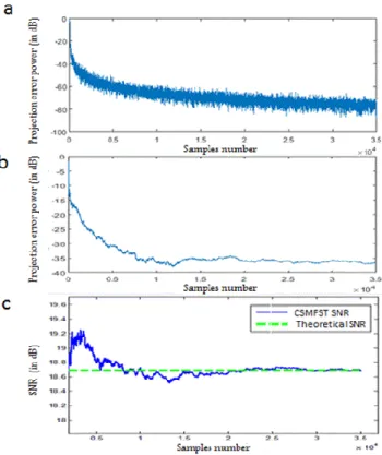
In all the simulations we choose 𝑛 = 8 and 𝑝 = 3.
The projection error power is the distance between the subspaces spanned by 𝑊1and 𝑊2[15] defined by
𝑑(𝑊1, 𝑊2) = ‖𝑊1𝑊1𝐻− 𝑊2𝑊2𝐻‖ 𝐹
A. Performance of the CSMFST algorithm in stationary case In this part, at each t, we compare the subspace returned by the CSMFST algorithm in a stationary case 𝑬𝒑(𝑡) with the one returned
by the OptSNR algorithm 𝑬𝒑∗(𝑡) then with the empirical subspace
𝒑 which is directly computed from all signal and noise samples. Since we are in a stationary case, the forgetting factor 𝛽 is chosen equal to 1.
In this first simulation all the eigenvectors of the signal covariance matrix 𝑪𝒙𝑨𝒙𝑨(𝑡) are considered to be fixed and three of the
corresponding eigenvalues 𝜆𝑖 are chosen larger than 1, however we
consider a white noise obtained by fixing a scalar noise matrix 𝑪𝒙𝑩𝒙𝑩(𝑡) with all eigenvalues 𝜇𝑖= 1.
Respectively, Fig. 1a and b represent the projection error powers i.e. the distance between 𝑬𝒑(𝑡) and 𝑬𝒑∗(𝑡) and between 𝑬𝒑(𝑡) and
𝒑.
It shows that the CSMFST algorithm presents a good rate of convergence as the resulting subspace returned by the algorithm 𝑬𝒑(𝑡) is close to 𝑬𝒑∗(𝑡) and also 𝒑.
Fig. 1c shows the difference between theoretical signal-to-noise ratio and the one computed by the CSMFST algorithm at each step, we can notice that they are quite similar
Since we are in a stationary case with a white noise, we can also compare the result obtained by the YAST on the signal samples and the CSMFST algorithm.
Fig. 2 presents the projection error power between the two algorithms.
In a second scenario, the eigenvectors 𝒖𝑖 of 𝑪𝒙𝑨𝒙𝑨(𝑡) and 𝑪𝒙𝑩𝒙𝑩(𝑡)
are the same.
The corresponding eigenvalues are chosen as following :
𝜆𝑖= [20,18,16,1,1,1,1,1] for the signal and 𝜇𝑖= [2,3,4,1,2,3,4,5] for
the noise.
It can be shown that the subspace returned by the algorithm 𝐸𝑝(𝑡) =
𝑠𝑝𝑎𝑛(𝑢1, 𝑢2, 𝑢4) with 𝜌 = 6.5, even though a fast and wrong analysis
would say 𝐸𝑝(𝑡) = 𝑠𝑝𝑎𝑛(𝑢1, 𝑢2, 𝑢3) where 𝜌 = 6.
Convincing results are given in fig. 3.
Fig. 1. Performance of the CSMFST algorithm in the stationary case in term of projection error power: the distance between 𝑬𝒑(𝑡) and 𝑬𝒑∗(𝑡) (a) and
between 𝑬𝒑(𝑡) and 𝒑 (b) and SNR(c).
Fig. 2. Comparison in stationary case between the YAST and the CSMFST in presence of white noise.
Fig. 3. Performance of the CSMFST algorithm in the stationary case.
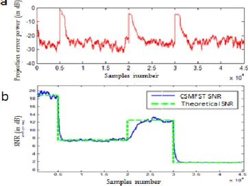
B. Performance of the CSMFST algorithm in nonstationary case
In this second part, we test the algorithm in a nonstationary environment with a forgetting factor 𝛽 equal to 0,999.
In this third scenario we keep the same eigenvectors of 𝑪𝒙𝑨𝒙𝑨(𝑡) and
the same white noise corresponding to the scalar matrix 𝑪𝒙𝑩𝒙𝑩(𝑡)
than the first scenario. However we create four different stationary zones in which we change the principal subspace by switching two eigenvectors of 𝑪𝒙𝑨𝒙𝑨(𝑡). In each zone we switch an eigenvector of
the principal subspace with another eigenvector chosen outside the principal subspace.
The signal-to-noise-ratio is constant.
Fig. 4a represents the distance between 𝑬𝒑(𝑡) and 𝑬𝒑∗(𝑡); we can
notice that the CSMFST algorithm presents a good convergence since the resulting subspace is quite near to 𝑬𝒑∗(𝑡) (we have exactly the
same result when we compare it to the empirical subspace). The same figure shows that we have some peaks obtained exactly at the beginning of each zone due to the subspace change.
In Fig. 4b we show the difference between theoretical and estimated signal-to-noise-ratio.
The Fourth scenario is the following: we create four zones in which we change the principal subspace by modifying the eigenvalues and the eigenvectors associated of 𝑪𝒙𝑨𝒙𝑨(𝑡) in each zone.
The signal-to-noise-ratio varies from a zone to another. The result can be seen on Fig. 5, we can observe that the SNR 𝜌(𝑡) is well estimated with a fast convergence rate.
Fig. 4. Performance of the CSMFST algorithm in the nonstationary case in term of projection error (a) and SNR (b).
Fig. 5. Performance of the CSMFST algorithm in the nonstationary case in term of projection error (a) and SNR (b).
The two last tests show that the CSMFST algorithm presents a good rate of convergence even in a nonstationary environment.
VI. CONCLUSION
In this paper, we present a new fast tracking algorithm which estimates at each step the p-dimensional subspace where the signal-to-noise ratio is maximal.
The main advantage of the CSMF algorithm is that it can be used not necessary in white noise environments while all the SP-type algorithms consider white noise.
The CSMFST algorithm estimates the covariance matrices as well as the optimal subspace at each time step using the signal and noise realizations and presents a good rate of convergence in stationary and nonstationary environments. In a non-white noise environment, it can be compared only with the optSNR algorithm which needs heavy calculations. In a white noise environment, it can be compared with classical SP-algorithms such as YAST.
REFERENCES
[1] A. J. V. D. Veen, E. F. Deprettere, et A. L. Swindlehurst, « Subspace-based signal analysis using singular value decomposition », Proceedings of the IEEE, vol. 81, no 9, p.
1277‑1308, sept. 1993.
[2] C. H. Bischof et G. M. Shroff, « On updating signal subspaces », IEEE Transactions on Signal Processing, vol. 40, no 1, p. 96‑105, janv. 1992.
[3] B. Yang, « Projection approximation subspace tracking », IEEE
Transactions on Signal Processing, vol. 43, no 1, p. 95‑107,
janv. 1995.
[4] K. Abed-Meraim, A. Chkeif, et Y. Hua, « Fast orthonormal PAST algorithm », IEEE Signal Processing Letters, vol. 7, no 3,
p. 60‑62, mars 2000.
[5] R. Badeau, B. David, et G. Richard, « Fast approximated power iteration subspace tracking », IEEE Transactions on Signal
Processing, vol. 53, no 8, p. 2931‑2941, août 2005.
[6] X. G. Doukopoulos et G. V. Moustakides, « Fast and Stable Subspace Tracking », IEEE Transactions on Signal Processing, vol. 56, no 4, p. 1452‑1465, avr. 2008.
[7] C. E. Davila, « Efficient, high performance, subspace tracking for time-domain data », IEEE Transactions on Signal
Processing, vol. 48, no 12, p. 3307‑3315, déc. 2000.
[8] R. Badeau, B. David, et G. Richard, « Yet Another Subspace Tracker », in International Conference on Acoustics, Speech,
and Signal Processing (ICASSP), Philadelphia, Pennsylvania,
United States, 2005, vol. 4, p. 329‑332.
[9] R. Badeau, B. David, et G. Richard, « YAST Algorithm for Minor Subspace Tracking », in International Conference on
Acoustics, Speech, and Signal Processing ICASSP’06,
Toulouse, France, 2006, vol. III, p. 552‑555.
[10] R. Badeau, G. Richard, et B. David, « Fast and stable YAST algorithm for principal and minor subspace tracking »,
IEEE_J_SP, vol. 56, no 8, p. 3437–3446, 2008.
[11] M. Arjomandi-Lari et M. Karimi, « Generalized YAST algorithm for signal subspace tracking », Signal Processing, vol. 117, p. 82‑95, déc. 2015.
[12] B. Borloz et B. Xerri, « Subspace SNR Maximization: The Constrained Stochastic Matched Filter », IEEE Transactions on
Signal Processing, vol. 59, no 4, p. 1346‑1355, avr. 2011.
[13] J.-F. Cavassilas et B. Xerri « A matched filter extension. Application in short signals detection degraded by noise », Traitement du signal, 1993, vol. 10, no 3, p. 215-221.
[14] B. Borloz, Estimation, détection, classification par
maximisation du rapport signal-à-bruit : le filtre adapté stochastique sous contrainte. Toulon, 2005.
[15] G. H. Golub et C. F. V. Loan, Matrix Computations, 3rd edition. Baltimore: Johns Hopkins University Press, 1996.